
Neural Networks in Trading: Injection of Global Information into Independent Channels (InjectTST)

Introduction
In recent years, Transformer-based architectures for multimodal time series forecasting have gained widespread popularity and are progressively becoming one of the most preferred models for time series analysis. Increasingly, models are utilizing independent channel approaches, where the model processes each channel sequence separately, without interacting with the others.
Channel independence offers two primary advantages:
- Noise Suppression: Independent models can focus on predicting individual channels without being influenced by noise from other channels.
- Mitigating Distribution Drift: Channel independence can help address the issue of distribution drift in time series.
Conversely, mixing channels tends to be less effective in dealing with these challenges, which can result in decreased model performance. However, channel mixing does have unique advantages:
- High Information Capacity: Channel mixing models excel at capturing inter-channel dependencies, potentially offering more information for forecasting future values.
- Channel Specificity: Optimizing multiple channels within channel mixing models allows the model to fully leverage the distinctive characteristics of each channel.
Moreover, since independent channel approaches analyze individual channels through a unified model, the model cannot distinguish between channels, focusing primarily on the shared patterns across multiple channels. This leads to a loss of channel specificity and may negatively impact multimodal time series forecasting.
Therefore, developing an effective model that combines the advantages of both channel independence and mixing — enabling the utilization of both approaches (noise reduction, mitigating distribution drift, high information capacity, and channel specificity) — is key to further enhancing multimodal time series forecasting performance.
However, building such a model presents a complex challenge. First, independent channel models are inherently at odds with channel dependencies. While fine-tuning a unified model for each channel can address channel specificity, it comes at a significant training cost. Secondly, existing noise reduction methods and solutions for distribution drift have yet to make channel mixing frameworks as robust as independent channel models.
One potential solution to these challenges is presented in the paper "InjectTST: A Transformer Method of Injecting Global Information into Independent Channels for Long Time Series Forecasting", which introduces a method for injecting global information into the individual channels of a multimodal time series (InjectTST). The authors of this method avoid explicitly modeling dependencies between channels for forecasting multimodal time series. Instead, they maintain the channel independence structure as the foundation, while selectively injecting global information (channel mixing) into each channel. This enables implicit channel mixing.
Each individual channel can selectively receive useful global information while avoiding noise, maintaining both high information capacity and noise suppression. Since channel independence is preserved as the base structure, distribution drift can also be mitigated.
Additionally, the authors incorporate a channel identifier into InjectTST to address the issue of channel specificity.
1. The InjectTST Algorithm
To generate forecasts Y for a given horizon T, we analyze historical values of a multimodal time series X, containing L time steps, with each time step represented as a vector of dimension M.
To solve this task using the advantages of both channel independence and mixing, the complex multi-level InjectTST algorithm is employed.
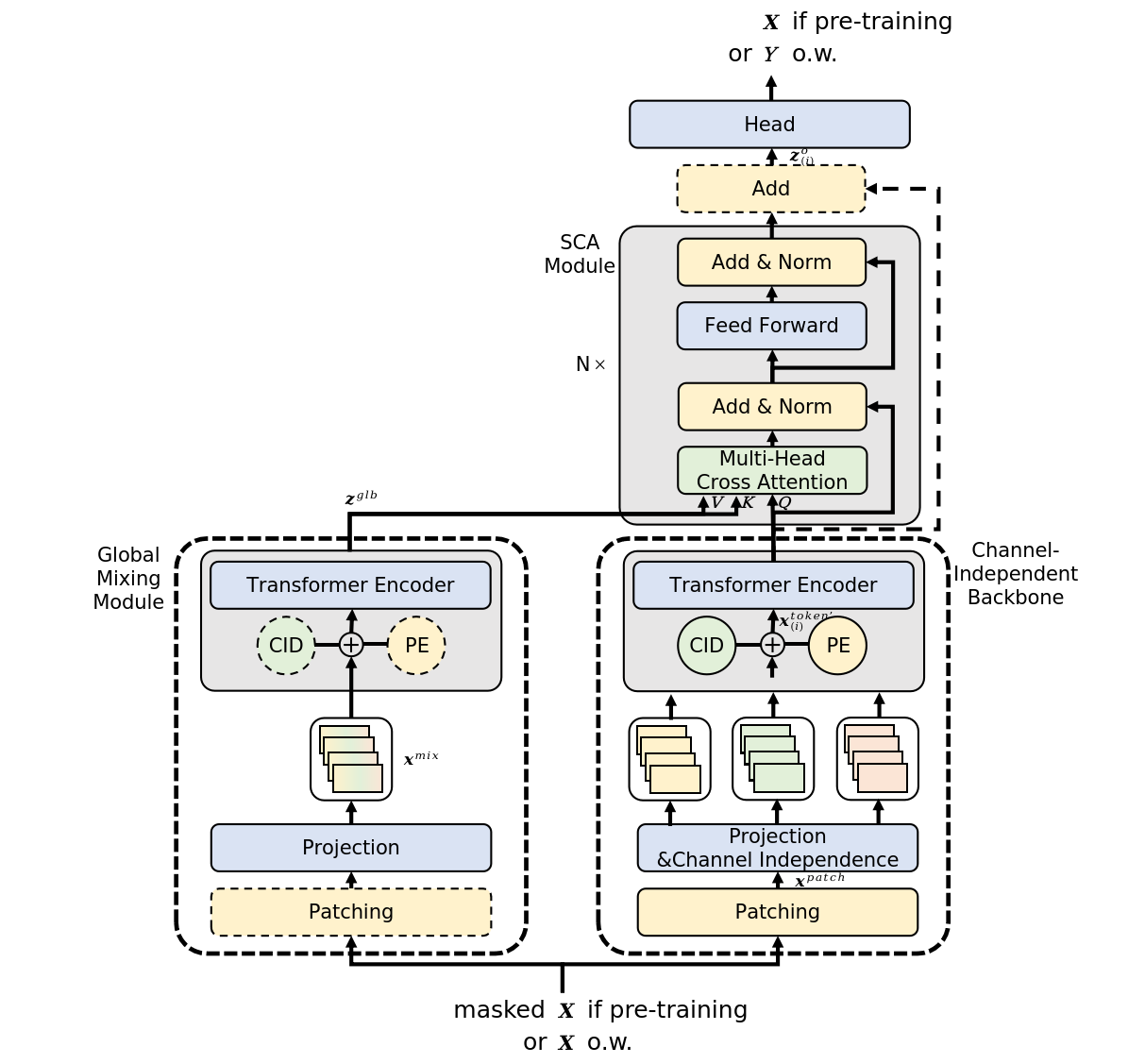
The first step of the algorithm involves segmenting the input data into independent channel highways. Afterward, a linear projection with learnable positional encoding is applied.
The independent channel platform processes each channel with a shared model. As a result, the model cannot differentiate between channels and primarily learns the common patterns of the channels, lacking channel specificity. To solve this, the authors of InjectTST introduce a channel identifier, which is a learnable tensor.
Following the linear projection of patches, tensors with both positional encoding and channel identifiers are added.
These prepared data are then fed into the Transformer encoder for high-level representation.
It is important to note that, in this case, the Transformer encoder operates in independent channel highways, meaning only the tokens of individual channels are analyzed, and there is no information exchange between channels.
The channel identifier represents the distinctive features of each channel, enabling the model to differentiate between them and obtain unique representations for each one.
Simultaneously, in parallel to the independent channel highway, the channel mixing route passes the original sequence X through a global mixing module to obtain global information. The main goal of InjectTST is to inject global information into each channel, making the retrieval of global information a critical task. The authors of the method propose two types of global mixing modules, referred to as CaT (Channel as Token) and PaT (Patch as Token).
The CaT module directly projects each channel into a token. In short, a linear projection is applied to all values within a channel.
The PaT global mixing module processes patches as input. Initially, patches related to the respective time steps of the analyzed multimodal sequence are grouped. A linear projection is then applied to the grouped patches, which primarily merges information at the patch level. Positional encoding is then added, and the data are passed to the Transformer encoder for further integration of information across patches and global information.
Experiments conducted by the authors indicate that PaT is more stable, whereas CaT performs better on certain specialized datasets.
A key challenge of the InjectTST method is the need to inject global information into each channel with minimal impact on the model's reliability. In a vanilla Transformer, cross-attention allows the target sequence to selectively focus on contextual information from another source based on relevance. This understanding of cross-attention architecture can also be applied to inject global information from multimodal time series. Therefore, global information, mixed across channels, can be treated as context. The authors use cross-attention for injecting global information into each channel.
It is worth noting that the authors introduce an optional residual connection for the contextual attention module. Typically, residual connections can make the model slightly unstable, but they can significantly improve performance on certain specialized datasets.
In general, global information is introduced into the contextual attention module as Key and Value, while channel-specific information is presented as Query.
After cross-attention, the data are enriched with global information. A linear head is added for generating forecast values.
InjectTST authors propose a three-stage training process. In the pre-training stage, the original time series are randomly masked, and the goal is to predict the masked parts. In the fine-tuning stage, the pre-trained InjectTST head is replaced with a forecasting head, and the forecasting head is fine-tuned, while the rest of the network is frozen. Finally, in the fine-tuning stage, the entire InjectTST network undergoes fine-tuning.
The original visualization of the method is shown below.
2. Implementing in MQL5
After reviewing the theoretical aspects of the InjectTST method, we proceed to the practical implementation of our interpretation of the proposed approaches using MQL5.
It is important to note that the implementation provided in this article is not the only correct one. Moreover, the proposed implementation reflects my personal understanding of the materials presented in the original paper and may differ from the authors' vision of the proposed approaches. The same applies to the results obtained.
When beginning work on the implementation of the proposed approaches, it is important to highlight that we have previously examined several Transformer-based models using the independent channel paradigm. In those models, forecasting was performed for independent channels, and the Transformer block was used to study inter-channel dependencies, which is akin to the CaT global mixing module approach.
However, the authors of the method employ a Transformer architecture in independent channel highways, avoiding the flow of information between channels at this stage. In theory, we could implement this algorithm by processing data in separate unitary sequences. However, this approach is extensive and leads to an increase in the number of sequential operations, which grows with the number of variables analyzed in multimodal input data.
In our work, we aim to perform as many operations as possible in parallel threads. Therefore, in this implementation, we will create a new layer that allows independent analysis of individual channels.
2.1 Independent Channel Analysis Block
The functionality for independent channel analysis is implemented in the class CNeuronMVMHAttentionMLKV, which inherits the basic functionality from another multi-layered multi-head attention block CNeuronMLMHAttentionOCL. The structure of the new class is shown below.
class CNeuronMVMHAttentionMLKV :  public CNeuronMLMHAttentionOCL
  {
protected:
   uint              iLayersToOneKV;       ///< Number of inner layers to 1 KV
   uint              iHeadsKV;             ///< Number of heads KV
   uint              iVariables;           ///< Number of variables
   CCollection       KV_Tensors;           ///< The collection of tensors of Keys and Values
   CCollection       K_Tensors;            ///< The collection of tensors of Keys
   CCollection       K_Weights;            ///< The collection of Matrix of K weights to previous layer
   CCollection       V_Tensors;            ///< The collection of tensors of Values
   CCollection       V_Weights;            ///< The collection of Matrix of V weights to previous layer
   CBufferFloat      Temp;
   //---
   virtual bool      feedForward(CNeuronBaseOCL *NeuronOCL) override;
   virtual bool      AttentionOut(CBufferFloat *q, CBufferFloat *kv, CBufferFloat *scores, CBufferFloat *out);
   virtual bool      AttentionInsideGradients(CBufferFloat *q, CBufferFloat *q_g,
                                              CBufferFloat *kv, CBufferFloat *kv_g,
                                              CBufferFloat *scores, CBufferFloat *gradient);
   //---
   virtual bool      calcInputGradients(CNeuronBaseOCL *prevLayer) override;
   virtual bool      updateInputWeights(CNeuronBaseOCL *NeuronOCL) override;

public:
                     CNeuronMVMHAttentionMLKV(void) {};
                    ~CNeuronMVMHAttentionMLKV(void) {};
   //---
   virtual bool      Init(uint numOutputs, uint myIndex, COpenCLMy *open_cl,
                          uint window, uint window_key, uint heads, uint heads_kv,
                          uint units_count, uint layers, uint layers_to_one_kv, uint variables,
                          ENUM_OPTIMIZATION optimization_type, uint batch);
   //---
   virtual int       Type(void)   const   {  return defNeuronMVMHAttentionMLKV;   }
   //---
   virtual bool      Save(int const file_handle);
   virtual bool      Load(int const file_handle);
   virtual bool      WeightsUpdate(CNeuronBaseOCL *source, float tau);
   virtual void      SetOpenCL(COpenCLMy *obj);
  };
In this class we add 3 variables:
- iLayersToOneKV — number of layers for 1 Key-Value tensor;
- iHeadsKV — number of attention heads in the Key-Value tensor;
- iVariables — the number of univariate sequences in a multimodal time series.
In addition, we add 5 data buffer collections, the purpose of which we will learn about as we go through the implementation. All internal objects are declared statically, which allows the class constructor and destructor to be left "empty". Initialization of all internal variables and objects is performed in the Init method.
bool CNeuronMVMHAttentionMLKV::Init(uint numOutputs, uint myIndex, COpenCLMy *open_cl,
                                    uint window, uint window_key, uint heads, uint heads_kv,
                                    uint units_count, uint layers, uint layers_to_one_kv, uint variables,
                                    ENUM_OPTIMIZATION optimization_type, uint batch)
  {
   if(!CNeuronBaseOCL::Init(numOutputs, myIndex, open_cl, window * units_count * variables,
                                                                   optimization_type, batch))
      return false;
In the parameters of this method we expect to receive the main constants that allow us to uniquely identify the architecture of the initialized class. These include:
- window — the size of the vector representing one element of the sequence of one univariate time series;
- window_key — the size of the vector of the internal representation of the Key entity of one element of the sequence of a univariate time series;
- heads — the number of attention heads of the Query entity;
- heads_kv — the number of attention heads in the concatenated Key-Value tensor;
- units_count — the size of the sequence being analyzed;
- layers — the number of nested layers in the block;
- layers_to_one_kv — the number of nested layers working with one Key-Vakue tensor;
- variables — the number of univariate sequences in a multimodal time series.
In the body of the method, we first call the same method of the parent class, which controls the received parameters and initializes the inherited objects. In addition, this method already implements the minimum necessary controls of data received from the caller.
After successful execution of the parent class method, we save the received parameters in internal variables.
   iWindow = fmax(window, 1);
   iWindowKey = fmax(window_key, 1);
   iUnits = fmax(units_count, 1);
   iHeads = fmax(heads, 1);
   iLayers = fmax(layers, 1);
   iHeadsKV = fmax(heads_kv, 1);
   iLayersToOneKV = fmax(layers_to_one_kv, 1);
   iVariables = variables;
Here we define the main constants that determine the architecture of nested objects.
   uint num_q = iWindowKey * iHeads * iUnits * iVariables;     //Size of Q tensor
   uint num_kv = iWindowKey * iHeadsKV * iUnits * iVariables;  //Size of KV tensor
   uint q_weights = (iWindow * iHeads + 1) * iWindowKey;       //Size of weights' matrix of Q tenzor
   uint kv_weights = (iWindow * iHeadsKV + 1) * iWindowKey;    //Size of weights' matrix of K/V tenzor
   uint scores = iUnits * iUnits * iHeads * iVariables;        //Size of Score tensor
   uint mh_out = iWindowKey * iHeads * iUnits * iVariables;    //Size of multi-heads self-attention
   uint out = iWindow * iUnits * iVariables;                   //Size of out tensore
   uint w0 = (iWindowKey * iHeads + 1) * iWindow;              //Size W0 weights' matrix
   uint ff_1 = 4 * (iWindow + 1) * iWindow;                    //Size of weights' matrix 1-st feed forward layer
   uint ff_2 = (4 * iWindow + 1) * iWindow;                    //Size of weights' matrix 2-nd feed forward layer
Here, it is important to briefly discuss the approaches we are proposing for the implementation within this class. First and foremost, a decision was made to construct the new class without modifying the OpenCL program. In other words, despite the new requirements, we are fully building the class using the existing kernels.
To achieve this, we start by separating the generation of the Key and Value entities. As a reminder, earlier they were generated in a single pass through the convolutional layer and written into the buffer sequentially for each sequence element. This approach is acceptable when constructing global attention. However, when organizing the process within separate channels, we would obtain an alternating sequence of Key/Value for individual channels, which is not ideal for subsequent analysis and does not fit well with the previously created algorithm. Therefore, we generate these entities separately and then concatenate them into a single tensor.
It is worth noting that we have divided the generation of entities into two stages, the number of which is independent of the number of analyzed variables or attention heads.
The second point is that the authors of the InjectTST method use a single Transformer encoder for all channels. Similarly, we use a single set of weight matrices for all channels. As a result, the size of the weight matrices remains constant, regardless of the number of channels.
With that, our preparatory work is complete, and we proceed to organize a loop with the number of iterations equal to the number of nested layers.
   for(uint i = 0; i < iLayers; i++)
     {
      CBufferFloat *temp = NULL;
In the loop body, we organize a nested loop to create buffers of the results of intermediate operations and the corresponding error gradients.
      for(int d = 0; d < 2; d++)
        {
         //--- Initilize Q tensor
         temp = new CBufferFloat();
         if(CheckPointer(temp) == POINTER_INVALID)
            return false;
         if(!temp.BufferInit(num_q, 0))
            return false;
         if(!temp.BufferCreate(OpenCL))
            return false;
         if(!QKV_Tensors.Add(temp))
            return false;
Here we first create the Query tensor buffer. The creation algorithm is identical for all buffers. First we create a new instance of the buffer object. We initialize it with zero values in a given size. Then we create a copy of the buffer in the OpenCL context and add a pointer to the buffer to the corresponding collection. Do not forget to control operations at each step.
Since we plan to use 1 Key-Value tensor for the analysis in several nested layers, we create the corresponding buffers with a given frequency.
         //--- Initilize KV tensor
         if(i % iLayersToOneKV == 0)
           {
            temp = new CBufferFloat();
            if(CheckPointer(temp) == POINTER_INVALID)
               return false;
            if(!temp.BufferInit(num_kv, 0))
               return false;
            if(!temp.BufferCreate(OpenCL))
               return false;
            if(!K_Tensors.Add(temp))
               return false;
            temp = new CBufferFloat();
            if(CheckPointer(temp) == POINTER_INVALID)
               return false;
            if(!temp.BufferInit(num_kv, 0))
               return false;
            if(!temp.BufferCreate(OpenCL))
               return false;
            if(!V_Tensors.Add(temp))
               return false;
            temp = new CBufferFloat();
            if(CheckPointer(temp) == POINTER_INVALID)
               return false;
            if(!temp.BufferInit(2 * num_kv, 0))
               return false;
            if(!temp.BufferCreate(OpenCL))
               return false;
            if(!KV_Tensors.Add(temp))
               return false;
           }
Note that at this stage we create 3 buffers: Key, Value and concatenated Key-Value.
The next step is to create a buffer of attention coefficients.
         //--- Initialize scores
         temp = new CBufferFloat();
         if(CheckPointer(temp) == POINTER_INVALID)
            return false;
         if(!temp.BufferInit(scores, 0))
            return false;
         if(!temp.BufferCreate(OpenCL))
            return false;
         if(!S_Tensors.Add(temp))
            return false;
Following this comes the buffer of results of multi-headed attention.
         //--- Initialize multi-heads attention out
         temp = new CBufferFloat();
         if(CheckPointer(temp) == POINTER_INVALID)
            return false;
         if(!temp.BufferInit(mh_out, 0))
            return false;
         if(!temp.BufferCreate(OpenCL))
            return false;
         if(!AO_Tensors.Add(temp))
            return false;
And then there are the compression buffers of the multi-headed attention and FeedForward block.
         //--- Initialize attention out
         temp = new CBufferFloat();
         if(CheckPointer(temp) == POINTER_INVALID)
            return false;
         if(!temp.BufferInit(out, 0))
            return false;
         if(!temp.BufferCreate(OpenCL))
            return false;
         if(!FF_Tensors.Add(temp))
            return false;
         //--- Initialize Feed Forward 1
         temp = new CBufferFloat();
         if(CheckPointer(temp) == POINTER_INVALID)
            return false;
         if(!temp.BufferInit(4 * out, 0))
            return false;
         if(!temp.BufferCreate(OpenCL))
            return false;
         if(!FF_Tensors.Add(temp))
            return false;
         //--- Initialize Feed Forward 2
         if(i == iLayers - 1)
           {
            if(!FF_Tensors.Add(d == 0 ? Output : Gradient))
               return false;
            continue;
           }
         temp = new CBufferFloat();
         if(CheckPointer(temp) == POINTER_INVALID)
            return false;
         if(!temp.BufferInit(out, 0))
            return false;
         if(!temp.BufferCreate(OpenCL))
            return false;
         if(!FF_Tensors.Add(temp))
            return false;
        }
After initializing the intermediate result buffers and their gradients, we move on to initializing the weight matrices. The algorithm for their initialization is similar to the creation of data buffers, only the matrix is filled with random values.
The first matrix generated is the weight matrix of the Query entity.
      //--- Initialize Q weights
      temp = new CBufferFloat();
      if(CheckPointer(temp) == POINTER_INVALID)
         return false;
      if(!temp.Reserve(q_weights))
         return false;
      float k = (float)(1 / sqrt(iWindow + 1));
      for(uint w = 0; w < q_weights; w++)
        {
         if(!temp.Add(GenerateWeight() * 2 * k - k))
            return false;
        }
      if(!temp.BufferCreate(OpenCL))
         return false;
      if(!QKV_Weights.Add(temp))
         return false;
Frequency of creation of weight matrices of Key and Value entities is similar to the frequency of the buffers of the corresponding entities.
      //--- Initialize K weights
      if(i % iLayersToOneKV == 0)
        {
         temp = new CBufferFloat();
         if(CheckPointer(temp) == POINTER_INVALID)
            return false;
         if(!temp.Reserve(kv_weights))
            return false;
         float k = (float)(1 / sqrt(iWindow + 1));
         for(uint w = 0; w < kv_weights; w++)
           {
            if(!temp.Add(GenerateWeight() * 2 * k - k))
               return false;
           }
         if(!temp.BufferCreate(OpenCL))
            return false;
         if(!K_Weights.Add(temp))
            return false;
         //---
         temp = new CBufferFloat();
         if(CheckPointer(temp) == POINTER_INVALID)
            return false;
         if(!temp.Reserve(kv_weights))
            return false;
         for(uint w = 0; w < kv_weights; w++)
           {
            if(!temp.Add(GenerateWeight() * 2 * k - k))
               return false;
           }
         if(!temp.BufferCreate(OpenCL))
            return false;
         if(!V_Weights.Add(temp))
            return false;
        }
Let's add a compression matrix of attention heads.
      //--- Initialize Weights0
      temp = new CBufferFloat();
      if(CheckPointer(temp) == POINTER_INVALID)
         return false;
      if(!temp.Reserve(w0))
         return false;
      for(uint w = 0; w < w0; w++)
        {
         if(!temp.Add(GenerateWeight() * 2 * k - k))
            return false;
        }
      if(!temp.BufferCreate(OpenCL))
         return false;
      if(!FF_Weights.Add(temp))
         return false;
And the FeedForward block.
      //--- Initialize FF Weights
      temp = new CBufferFloat();
      if(CheckPointer(temp) == POINTER_INVALID)
         return false;
      if(!temp.Reserve(ff_1))
         return false;
      for(uint w = 0; w < ff_1; w++)
        {
         if(!temp.Add(GenerateWeight() * 2 * k - k))
            return false;
        }
      if(!temp.BufferCreate(OpenCL))
         return false;
      if(!FF_Weights.Add(temp))
         return false;
      //---
      temp = new CBufferFloat();
      if(CheckPointer(temp) == POINTER_INVALID)
         return false;
      if(!temp.Reserve(ff_2))
         return false;
      k = (float)(1 / sqrt(4 * iWindow + 1));
      for(uint w = 0; w < ff_2; w++)
        {
         if(!temp.Add(GenerateWeight() * 2 * k - k))
            return false;
        }
      if(!temp.BufferCreate(OpenCL))
         return false;
      if(!FF_Weights.Add(temp))
         return false;
After that, we will create another nested loop in which we will add moment buffers at the weight coefficient level. The number of buffers created depends on the parameter update method.
      for(int d = 0; d < (optimization == SGD ? 1 : 2); d++)
        {
         temp = new CBufferFloat();
         if(CheckPointer(temp) == POINTER_INVALID)
            return false;
         if(!temp.BufferInit((d == 0 || optimization == ADAM ? q_weights : iWindowKey * iHeads), 0))
            return false;
         if(!temp.BufferCreate(OpenCL))
            return false;
         if(!QKV_Weights.Add(temp))
            return false;
         if(i % iLayersToOneKV == 0)
           {
            temp = new CBufferFloat();
            if(CheckPointer(temp) == POINTER_INVALID)
               return false;
            if(!temp.BufferInit((d == 0 || optimization == ADAM ? kv_weights : iWindowKey * iHeadsKV), 0))
               return false;
            if(!temp.BufferCreate(OpenCL))
               return false;
            if(!K_Weights.Add(temp))
               return false;
            //---
            temp = new CBufferFloat();
            if(CheckPointer(temp) == POINTER_INVALID)
               return false;
            if(!temp.BufferInit((d == 0 || optimization == ADAM ? kv_weights : iWindowKey * iHeadsKV), 0))
               return false;
            if(!temp.BufferCreate(OpenCL))
               return false;
            if(!V_Weights.Add(temp))
               return false;
           }
         temp = new CBufferFloat();
         if(CheckPointer(temp) == POINTER_INVALID)
            return false;
         if(!temp.BufferInit((d == 0 || optimization == ADAM ? w0 : iWindow), 0))
            return false;
         if(!temp.BufferCreate(OpenCL))
            return false;
         if(!FF_Weights.Add(temp))
            return false;
         //--- Initilize FF Weights
         temp = new CBufferFloat();
         if(CheckPointer(temp) == POINTER_INVALID)
            return false;
         if(!temp.BufferInit((d == 0 || optimization == ADAM ? ff_1 : 4 * iWindow), 0))
            return false;
         if(!temp.BufferCreate(OpenCL))
            return false;
         if(!FF_Weights.Add(temp))
            return false;
         temp = new CBufferFloat();
         if(CheckPointer(temp) == POINTER_INVALID)
            return false;
         if(!temp.BufferInit((d == 0 || optimization == ADAM ? ff_2 : iWindow), 0))
            return false;
         if(!temp.BufferCreate(OpenCL))
            return false;
         if(!FF_Weights.Add(temp))
            return false;
        }
     }
At the end of the initialization method, we add a buffer to store temporary data and return the logical result of the operations performed to the calling program.
   if(!Temp.BufferInit(MathMax(2 * num_kv, out), 0))
      return false;
   if(!Temp.BufferCreate(OpenCL))
      return false;
//---
   return true;
  }
After initializing the object, we move on to organizing the forward pass algorithms. And here a few words are worth saying about the use of previously created kernels. In particular, about the feed-forward pass kernel of the cross-attention block MH2AttentionOut, the algorithm for placing it in the execution queue is implemented in the AttentionOut method. The algorithm for placing the kernel in the execution queue has not changed. But our task is to implement the analysis of independent channels using this algorithm.
First, let's look at how our kernel works with individual attention heads. It processes them independently in separate streams. I think this is exactly what we need. So let's say that individual channels are the same attention heads.
bool CNeuronMVMHAttentionMLKV::AttentionOut(CBufferFloat *q, CBufferFloat *kv,
                                            CBufferFloat *scores, CBufferFloat *out)
  {
   if(!OpenCL)
      return false;
//---
   uint global_work_offset[3] = {0};
   uint global_work_size[3] = {iUnits/*Q units*/, iUnits/*K units*/, iHeads * iVariables};
   uint local_work_size[3] = {1, iUnits, 1};
Otherwise, the algorithm of the method remains the same. Let's pass the necessary parameters to the kernel.
   ResetLastError();
   if(!OpenCL.SetArgumentBuffer(def_k_MH2AttentionOut, def_k_mh2ao_q, q.GetIndex()))
     {
      printf("Error of set parameter kernel %s: %d; line %d", __FUNCTION__, GetLastError(), __LINE__);
      return false;
     }
   if(!OpenCL.SetArgumentBuffer(def_k_MH2AttentionOut, def_k_mh2ao_kv, kv.GetIndex()))
     {
      printf("Error of set parameter kernel %s: %d; line %d", __FUNCTION__, GetLastError(), __LINE__);
      return false;
     }
   if(!OpenCL.SetArgumentBuffer(def_k_MH2AttentionOut, def_k_mh2ao_score, scores.GetIndex()))
     {
      printf("Error of set parameter kernel %s: %d; line %d", __FUNCTION__, GetLastError(), __LINE__);
      return false;
     }
   if(!OpenCL.SetArgumentBuffer(def_k_MH2AttentionOut, def_k_mh2ao_out, out.GetIndex()))
     {
      printf("Error of set parameter kernel %s: %d; line %d", __FUNCTION__, GetLastError(), __LINE__);
      return false;
     }
   if(!OpenCL.SetArgument(def_k_MH2AttentionOut, def_k_mh2ao_dimension, (int)iWindowKey))
     {
      printf("Error of set parameter kernel %s: %d; line %d", __FUNCTION__, GetLastError(), __LINE__);
      return false;
     }
Adjust the number of Key-Value tensor heads.
   if(!OpenCL.SetArgument(def_k_MH2AttentionOut, def_k_mh2ao_heads_kv, (int)(iHeadsKV * iVariables)))
     {
      printf("Error of set parameter kernel %s: %d; line %d", __FUNCTION__, GetLastError(), __LINE__);
      return false;
     }
Then put the kernel in the execution queue.
   if(!OpenCL.SetArgument(def_k_MH2AttentionOut, def_k_mh2ao_mask, 0))
     {
      printf("Error of set parameter kernel %s: %d; line %d", __FUNCTION__, GetLastError(), __LINE__);
      return false;
     }
   if(!OpenCL.Execute(def_k_MH2AttentionOut, 3, global_work_offset, global_work_size, local_work_size))
     {
      printf("Error of execution kernel %s: %d", __FUNCTION__, GetLastError());
      return false;
     }
//---
   return true;
  }
This finishes the method. But this is only part of the feed-forward pass algorithm. We will build the complete algorithm in the feedForward method.
bool CNeuronMVMHAttentionMLKV::feedForward(CNeuronBaseOCL *NeuronOCL)
  {
   if(CheckPointer(NeuronOCL) == POINTER_INVALID)
      return false;
In the parameters, the method receives a pointer to the object of the previous neural layer, which contains the initial data for our algorithm. As the initial data we expect to receive a three-dimensional tensor - the length of the sequence * the number of univariate sequences * the size of the analyzed window of one element.
In the body of the method, we check the relevance of the received pointer and organize a cycle of iterating through the nested layers of the module.
   CBufferFloat *kv = NULL;
   for(uint i = 0; (i < iLayers && !IsStopped()); i++)
     {
      //--- Calculate Queries, Keys, Values
      CBufferFloat *inputs = (i == 0 ? NeuronOCL.getOutput() : FF_Tensors.At(6 * i - 4));
Here we first declare a local pointer to the source data buffer into which we will store the required pointer. After that, we extract from the collection the Query entity buffer corresponding to the analyzed layer and write into it the data generated based on the original data.
      CBufferFloat *q = QKV_Tensors.At(i * 2);
      if(IsStopped() ||
        !ConvolutionForward(QKV_Weights.At(i * (optimization == SGD ? 2 : 3)), inputs, q,
                                                       iWindow, iWindowKey * iHeads, None))
         return false;
The next step we will check is the need to generate a new Key-Value tensor. If necessary, we will first determine the offset in the relevant collections.
      if((i % iLayersToOneKV) == 0)
        {
         uint i_kv = i / iLayersToOneKV;
And we extract pointers to the buffers we need.
         kv = KV_Tensors.At(i_kv * 2);
         CBufferFloat *k = K_Tensors.At(i_kv * 2);
         CBufferFloat *v = V_Tensors.At(i_kv * 2);
After which we will sequentially generate Key and Value entities.
         if(IsStopped() ||
            !ConvolutionForward(K_Weights.At(i_kv * (optimization == SGD ? 2 : 3)), inputs, k,
                                                            iWindow, iWindowKey * iHeadsKV, None))
            return false;
         if(IsStopped() ||
            !ConvolutionForward(V_Weights.At(i_kv * (optimization == SGD ? 2 : 3)), inputs, v,
                                                            iWindow, iWindowKey * iHeadsKV, None))
            return false;
And we concatenate the obtained tensors along the first dimension (elements of the sequence).
         if(IsStopped() ||
            !Concat(k, v, kv, iWindowKey * iHeadsKV * iVariables, iWindowKey * iHeadsKV * iVariables, iUnits))
            return false;
        }
Please note that in this version of data organization we get a data buffer, which can be represented as a five-dimensional data tensor: Units * [Key, Value] * Variable * HeadsKV * Window_Key. Query entity tensor has a comparable dimension, only instead of [Key, Value] we have [Query]. By aggregating the dimensions of Variable and Heads in one dimension "Variable * Heads", we get tensor dimensions comparable to vanilla Multi-Heads Self-Attention.
Here it is necessary to remind that on the OpenCL context side we work with one-dimensional data buffers. Splitting the data into a multidimensional tensor is only declarative for understanding the sequence of data. In general, the sequence of data in the buffer goes from the last dimension to the first.
This allows us to use previously created kernels of our OpenCL program for analyzing independent channels. We get pointers to the required data buffers from the collections and execute the Multi-Heads Self-Attention algorithm. We have adjusted the required method above.
      //--- Score calculation and Multi-heads attention calculation
      CBufferFloat *temp = S_Tensors.At(i * 2);
      CBufferFloat *out = AO_Tensors.At(i * 2);
      if(IsStopped() || !AttentionOut(q, kv, temp, out))
         return false;
We then mentally reformat the results of multi-headed attention into a tensor of [Units * Variable] * Heads * Window_Key and project the data to the dimension of the original data.
      //--- Attention out calculation
      temp = FF_Tensors.At(i * 6);
      if(IsStopped() ||
         !ConvolutionForward(FF_Weights.At(i * (optimization == SGD ? 6 : 9)), out, temp,
                                                       iWindowKey * iHeads, iWindow, None))
         return false;
      //--- Sum and normilize attention
      if(IsStopped() || !SumAndNormilize(temp, inputs, temp, iWindow, true))
         return false;
After which we sum the obtained results with the original data and normalize the obtained values.
Next, we perform the FeedForward block operations in the same style and move on to the next iteration of the loop.
      //--- Feed Forward
      inputs = temp;
      temp = FF_Tensors.At(i * 6 + 1);
      if(IsStopped() ||
         !ConvolutionForward(FF_Weights.At(i * (optimization == SGD ? 6 : 9) + 1), inputs, temp,
                                                                     iWindow, 4 * iWindow, LReLU))
         return false;
      out = FF_Tensors.At(i * 6 + 2);
      if(IsStopped() ||
         !ConvolutionForward(FF_Weights.At(i * (optimization == SGD ? 6 : 9) + 2), temp, out,
                                                                 4 * iWindow, iWindow, activation))
         return false;
      //--- Sum and normilize out
      if(IsStopped() || !SumAndNormilize(out, inputs, out, iWindow, true))
         return false;
     }
//---
   return true;
  }
After successfully completing the operations of all nested layers within the block, we finalize the method's execution and return a logical result to the calling program, indicating the completion status of the operations.
Typically, after implementing the feed-forward pass methods, we proceed to developing the backpropagation algorithms. Today, I would like to invite you to independently analyze the proposed implementation, which you will find in the attached materials. In the process of implementing the backpropagation methods, we utilized the same approaches described earlier for the feed-forward pass. It is important to note that backpropagation operations strictly follow the forward pass algorithm but in reverse order.
Additionally, the attachment contains the implementation of the CNeuronMVCrossAttentionMLKV class, whose algorithms largely mirror those of the CNeuronMVMHAttentionMLKV class, with the key addition of cross-attention mechanisms.
I would also like to remind you that the implemented classes, CNeuronMVMHAttentionMLKV and CNeuronMVCrossAttentionMLKV, serve as building blocks within the larger InjectTST algorithm, the theoretical aspects of which we explored earlier. The next step in our work will be to develop a new class where we will implement the full InjectTST algorithm.
2.2 Implementation of InjectTST
We will construct the complete InjectTST algorithm within the CNeuronInjectTST class, which will inherit the core functionality from the parent class of fully connected neural layers, CNeuronBaseOCL. The structure of the new class is shown below.
class CNeuronInjectTST  :  public CNeuronBaseOCL
  {
protected:
   CNeuronPatching            cPatching;
   CNeuronLearnabledPE        cCIPosition;
   CNeuronLearnabledPE        cCMPosition;
   CNeuronMVMHAttentionMLKV   cChanelIndependentAttention;
   CNeuronMLMHAttentionMLKV   cChanelMixAttention;
   CNeuronMVCrossAttentionMLKV   cGlobalInjectionAttention;
   CBufferFloat               cTemp;
   //---
   virtual bool      feedForward(CNeuronBaseOCL *NeuronOCL) override;
   //---
   virtual bool      calcInputGradients(CNeuronBaseOCL *NeuronOCL) override;
   virtual bool      updateInputWeights(CNeuronBaseOCL *NeuronOCL) override;
   //---

public:
                     CNeuronInjectTST(void) {};
                    ~CNeuronInjectTST(void) {};
   //---
   virtual bool      Init(uint numOutputs, uint myIndex, COpenCLMy *open_cl,
                          uint window, uint window_key, uint heads, uint heads_kv,
                          uint units_count, uint layers, uint layers_to_one_kv,
                          uint variables, ENUM_OPTIMIZATION optimization_type, uint batch);
   //---
   virtual int       Type(void)   const   {  return defNeuronInjectTST; }
   //---
   virtual bool      Save(int const file_handle);
   virtual bool      Load(int const file_handle);
   //---
   virtual bool      WeightsUpdate(CNeuronBaseOCL *source, float tau);
   virtual void      SetOpenCL(COpenCLMy *obj);
   //---
   virtual CBufferFloat   *getWeights(void)  override;
  };
In this class we see quite a large number of internal objects, but there is not a single variable. This is due to the fact that this class implements, one might say, a "large-node assembly" of an algorithm, the main functionality of which is built by internal objects. And all constants that define the block architecture are used only in the class initialization method and are stored inside nested objects. We will become familiar with the functionality of these in the process of implementing the algorithms.
All internal objects of the class are declared statically, which allows us to leave the class constructor and destructor empty. And the initialization of all nested and inherited objects is carried out in the Init method.
bool CNeuronInjectTST::Init(uint numOutputs, uint myIndex, COpenCLMy *open_cl,
                            uint window, uint window_key, uint heads, uint heads_kv,
                            uint units_count, uint layers, uint layers_to_one_kv,
                            uint variables, ENUM_OPTIMIZATION optimization_type, uint batch)
  {
   if(!CNeuronBaseOCL::Init(numOutputs, myIndex, open_cl, window * units_count * variables,
                                                                   optimization_type, batch))
      return false;
   SetActivationFunction(None);
As usual, in the parameters of this method we receive the main constants that determine the architecture of the created object. In the body of the method, we immediately call the method of the same name of the parent class, which already implements basic controls for the received parameters and initialization of inherited objects.
Next, we initialize the internal objects in the forward pass sequence of the InjectTST algorithm. In the author's visualization of the method presented above, it is easy to see that the obtained initial data is used in 2 information flows: blocks of independent channels and global mixing. In both blocks, the source data is first segmented. In my implementation, I decided not to duplicate the segmentation process, but to carry it out once before the information flows branched.
   if(!cPatching.Init(0, 0, OpenCL, window, window, window, units_count, variables, optimization, iBatch))
      return false;
   cPatching.SetActivationFunction(None);
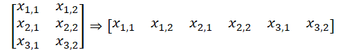
It should be noted that in this implementation I use equal parameters: segment size, segment window step, and segment embedding size. Thus, the size of the source data buffer before and after segmentation did not change. However, the sequence of data in the buffer has changed. The data tensor from two dimensions L * V was reformatted into three dimensions L/p * V * p, where L is the length of the multimodal sequence of initial data, V is the number of variables analyzed, and p is segment size.
To the segment tokens in the block of the independent channel trunk, the authors of the method add two trainable tensors: positional coding and channel identification. The sum of 2 numbers is a number, so in my implementation I decided to use a single learnable positional encoding layer that learns the positional label of each individual element in the input tensor.
   if(!cCIPosition.Init(0, 1, OpenCL, window * units_count * variables, optimization, iBatch))
      return false;
   cCIPosition.SetActivationFunction(None);
In the global mixing block, the algorithm also provides positional coding. We initialize a similar layer for the second information flow highway.
   if(!cCMPosition.Init(0, 2, OpenCL, window * units_count * variables, optimization, iBatch))
      return false;
   cCMPosition.SetActivationFunction(None);
We will construct the independent channel backbone using the independent channel CNeuronMVMHAttentionMLKV attention block discussed above.
   if(!cChanelIndependentAttention.Init(0, 3, OpenCL, window, window_key, heads, heads_kv, units_count,
                                              layers, layers_to_one_kv, variables, optimization, iBatch))
      return false;
   cChanelIndependentAttention.SetActivationFunction(None);
And to organize the global mixing block, we will use the previously created attention block CNeuronMLMHAttentionMLKV.
   if(!cChanelMixAttention.Init(0, 4, OpenCL, window * variables, window_key, heads, heads_kv, units_count,
                                                             layers, layers_to_one_kv, optimization, iBatch))
      return false;
   cChanelMixAttention.SetActivationFunction(None);
Note that in this case the window size of the analyzed vector of one element is equal to the product of the segment size and the number of analyzed variables, which corresponds to the channel mixing paradigm.
The injection of global information into independent channels is carried out within the cross-attention block.
   if(!cGlobalInjectionAttention.Init(0, 5, OpenCL, window, window_key, heads, window * variables, heads_kv,
                                      units_count, units_count, layers, layers_to_one_kv, variables, 1,
                                      optimization, iBatch))
      return false;
   cGlobalInjectionAttention.SetActivationFunction(None);
Note that in this case we set the number of unitary rows in the context to 1, since we are working with mixed channels here.
At the end of the initialization method, we perform a swap of data buffers, which will allow us to avoid unnecessary copying between the buffers of our class and internal objects.
   if(!SetOutput(cGlobalInjectionAttention.getOutput(), true) ||
      !SetGradient(cGlobalInjectionAttention.getGradient(), true)
     )
      return false;
We initialize an auxiliary buffer for storing intermediate data and return the logical result of the operations to the calling program.
   if(!cTemp.BufferInit(cPatching.Neurons(), 0) ||
      !cTemp.BufferCreate(OpenCL)
     )
      return false;
//---
   return true;
  }
After initializing the class object, we move on to building the feed-forward pass algorithm for our class. We have already discussed the main stages of the algorithm in the process of implementing the initialization method. And now we just have to describe them in the feedForward method.
bool CNeuronInjectTST::feedForward(CNeuronBaseOCL *NeuronOCL)
  {
   if(!cPatching.FeedForward(NeuronOCL))
      return false;
In the method parameters we receive a pointer to the object of the previous layer, which passes us the original data. We immediately pass the received pointer to the method of the nested data segmentation layer with the same name.
Note that at this stage we do not check the relevance of the obtained pointer, since the necessary controls are implemented in the segmentation layer method and re-checking would be unnecessary.
The next step is to add positional encoding to the segmented data.
   if(!cCIPosition.FeedForward(cPatching.AsObject()) ||
      !cCMPosition.FeedForward(cPatching.AsObject())
     )
      return false;
After which we first pass the data through a block of independent channels.
   if(!cChanelIndependentAttention.FeedForward(cCIPosition.AsObject()))
      return false;
And then through the global mixing block.
   if(!cChanelMixAttention.FeedForward(cCMPosition.AsObject()))
      return false;
Please note that despite the sequence of execution, these are 2 independent streams of information. Only in the contextual attention block is the injection of global data into independent channels carried out.
   if(!cGlobalInjectionAttention.FeedForward(cCIPosition.AsObject(), cCMPosition.getOutput()))
      return false;
//---
   return true;
  }
We moved the decision-making process outside the CNeuronInjectTST class.
As you can see, the feed-forward pass method turned out to be quite concise and readable. In other words, as expected from a large-node implementation of the algorithm. Backward pass methods are constructed in a similar way. You can find the code them yourself in the attachment. The full code of this class and all its methods is presented in the attachment. The attachment also contains complete code for all programs used in the article.
2.3 Architecture of Trainable Models
Above we have implemented the basic algorithms of the InjectTST method by meansMQL5 and now we can implement the proposed approaches into our own models. The method we are considering was proposed for forecasting time series. And we, similar to a number of previously considered methods for forecasting time series, will try to implement the proposed approaches into the Environmental State Encoder model. As you know, the description of the architecture of this model is presented in the CreateEncoderDescriptions method.
bool CreateEncoderDescriptions(CArrayObj *&encoder)
  {
//---
   CLayerDescription *descr;
//---
   if(!encoder)
     {
      encoder = new CArrayObj();
      if(!encoder)
         return false;
     }
In the parameters of this method we receive a pointer to a dynamic array object for recording the model architecture. In the body of the method, we immediately check the relevance of the received pointer and, if necessary, create a new dynamic array object. And then we begin to describe the architecture of the model being created.
The first is the basic fully connected layer, which is used to record the original data.
//--- Input layer
   if(!(descr = new CLayerDescription()))
      return false;
   descr.type = defNeuronBaseOCL;
   int prev_count = descr.count = (HistoryBars * BarDescr);
   descr.activation = None;
   descr.optimization = ADAM;
   if(!encoder.Add(descr))
     {
      delete descr;
      return false;
     }
As always, we plan to feed the model with raw input data. And they undergo primary processing in the batch data normalization layer, where information from different distributions is brought into a comparable form.
//--- layer 1
   if(!(descr = new CLayerDescription()))
      return false;
   descr.type = defNeuronBatchNormOCL;
   descr.count = prev_count;
   descr.batch = 1e4;
   descr.activation = None;
   descr.optimization = ADAM;
   if(!encoder.Add(descr))
     {
      delete descr;
      return false;
     }
Next up is our new layer of independent channels with global injection.
//--- layer 2
   if(!(descr = new CLayerDescription()))
      return false;
   descr.type = defNeuronInjectTST;
   descr.window = PatchSize;                                      //Patch window
   descr.window_out = 8;                                          //Window Key
To specify the segment size we add the PatchSize constant. We calculate the size of the sequence based on the depth of the analyzed history and the size of the segment.
   prev_count = descr.count =
                   (HistoryBars + descr.window - 1) / descr.window; //Units
Number of attention heads for Query, Key and Value entities, and we will also write the number of unitary sequences into an array.
     {
      int temp[] =
        {
         4,                                                       //Heads
         2,                                                       //Heads KV
         BarDescr                                                 //Variables
        };
      ArrayCopy(descr.heads, temp);
     }
All internal blocks will contain 4 folded layers.
descr.layers = 4; //Layers
And one Key-Value tensor will be relevant for 2 nested layers.
   descr.step = 2;                                                //Layers to 1 KV
   descr.batch = 1e4;
   descr.activation = None;
   descr.optimization = ADAM;
   if(!encoder.Add(descr))
     {
      delete descr;
      return false;
     }
Next we need to add a head for predicting subsequent values. We remember that at the output of the InjectTST block we get a tensor of dimensionL/p * V * p. And in order to make a forecast of data within independent channels, we first need to transpose the data.
//--- layer 3
   if(!(descr = new CLayerDescription()))
      return false;
   descr.type = defNeuronTransposeOCL;
   descr.count = prev_count;
   descr.window = PatchSize * BarDescr;
   descr.activation = None;
   descr.optimization = ADAM;
   if(!encoder.Add(descr))
     {
      delete descr;
      return false;
     }
Then we use two-layer MLP to predict independent channels.
//--- layer 4
   if(!(descr = new CLayerDescription()))
      return false;
   descr.type = defNeuronConvOCL;
   descr.count = PatchSize * BarDescr;
   descr.window = prev_count;
   descr.window_out = NForecast;
   descr.activation = LReLU;
   descr.optimization = ADAM;
   if(!encoder.Add(descr))
     {
      delete descr;
      return false;
     }
//--- layer 5
   if(!(descr = new CLayerDescription()))
      return false;
   descr.type = defNeuronConvOCL;
   descr.count = BarDescr;
   descr.window = PatchSize * NForecast;
   descr.window_out = NForecast;
   descr.activation = TANH;
   descr.optimization = ADAM;
   if(!encoder.Add(descr))
     {
      delete descr;
      return false;
     }
In doing so, we reduce the dimensionality of the data down to Variables * Forecast. Now we can return the predicted values to the original data representation.
//--- layer 6
   if(!(descr = new CLayerDescription()))
      return false;
   descr.type = defNeuronTransposeOCL;
   descr.count = BarDescr;
   descr.window = NForecast;
   descr.activation = None;
   descr.optimization = ADAM;
   if(!encoder.Add(descr))
     {
      delete descr;
      return false;
     }
We add statistical indicators removed from the original data during normalization.
//--- layer 7
   if(!(descr = new CLayerDescription()))
      return false;
   descr.type = defNeuronRevInDenormOCL;
   descr.count = BarDescr * NForecast;
   descr.activation = None;
   descr.optimization = ADAM;
   descr.layers = 1;
   if(!encoder.Add(descr))
     {
      delete descr;
      return false;
     }
In addition, we use the approaches of the FreDF method to align the predicted values of univariate series in the frequency domain.
//--- layer 8
   if(!(descr = new CLayerDescription()))
      return false;
   descr.type = defNeuronFreDFOCL;
   descr.window = BarDescr;
   descr.count =  NForecast;
   descr.step = int(true);
   descr.probability = 0.7f;
   descr.activation = None;
   descr.optimization = ADAM;
   if(!encoder.Add(descr))
     {
      delete descr;
      return false;
     }
//---
   return true;
  }
I use the architectures of the Actor and Critic models from previous works. Therefore, we will not dwell on their description in detail now.
Moreover, in the new Encoder architecture, we did not change either the source data layer or the results to determine the account status. All this allows us to use all previously created programs for interacting with the environment and training models without any changes. Accordingly, we can use the previously collected training sample for the initial training of models.
You can find the full code of all classes and their methods, as well as all programs used in preparing the article, in the attachment.
3. Testing
Above, we implemented the InjectTST method using MQL5 and demonstrated its application in the Environmental State Encoder model. Now, we proceed to evaluating the model’s effectiveness on real historical data.
As before, we first train the Environmental State Encoder model to predict future price movements over a specified forecast horizon. In this experiment, the training dataset consists of historical data from 2023 for the EURUSD instrument on the H1 timeframe.
The Environmental State Encoder analyzes only historical price data, which is not influenced by the Agent's actions. Thus, we train the model until we achieve satisfactory results or the forecasting error plateaus.
Below is a comparative visualization of the predicted and actual price movement trajectories.
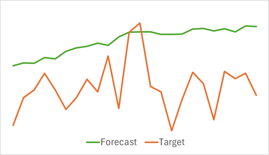
As shown in the graph, the predicted trajectory is shifted upwards and exhibits less pronounced fluctuations. However, the overall trend direction aligns with the target trajectory. While this may not be the most accurate forecast compared to previously explored models, we move on to the second phase of training to assess whether this Encoder can help the Actor develop a profitable strategy.
Training the Actor and Critic models is performed iteratively. Initially, we conduct several epochs of model training using the existing training dataset. Then, during interaction with the environment, we update the dataset based on rewards obtained from actions under the Actor's current policy. This allows us to enrich the training set with real action rewards from the current Actor policy distribution. This enrichment of the training dataset with real reward values allows for better optimization of the Critic's reward function and more precise evaluation of the Actor's actions. This, in turn, enables adjustments to improve the current policy’s effectiveness. The iterations continue until the desired outcome is achieved.
To assess the effectiveness of the trained Actor’s policy, we conduct a test run of the environment interaction advisor within the MetaTrader 5 strategy tester. Testing is performed on historical data from January 2024 while keeping all other parameters unchanged. The results of the test run are presented below.
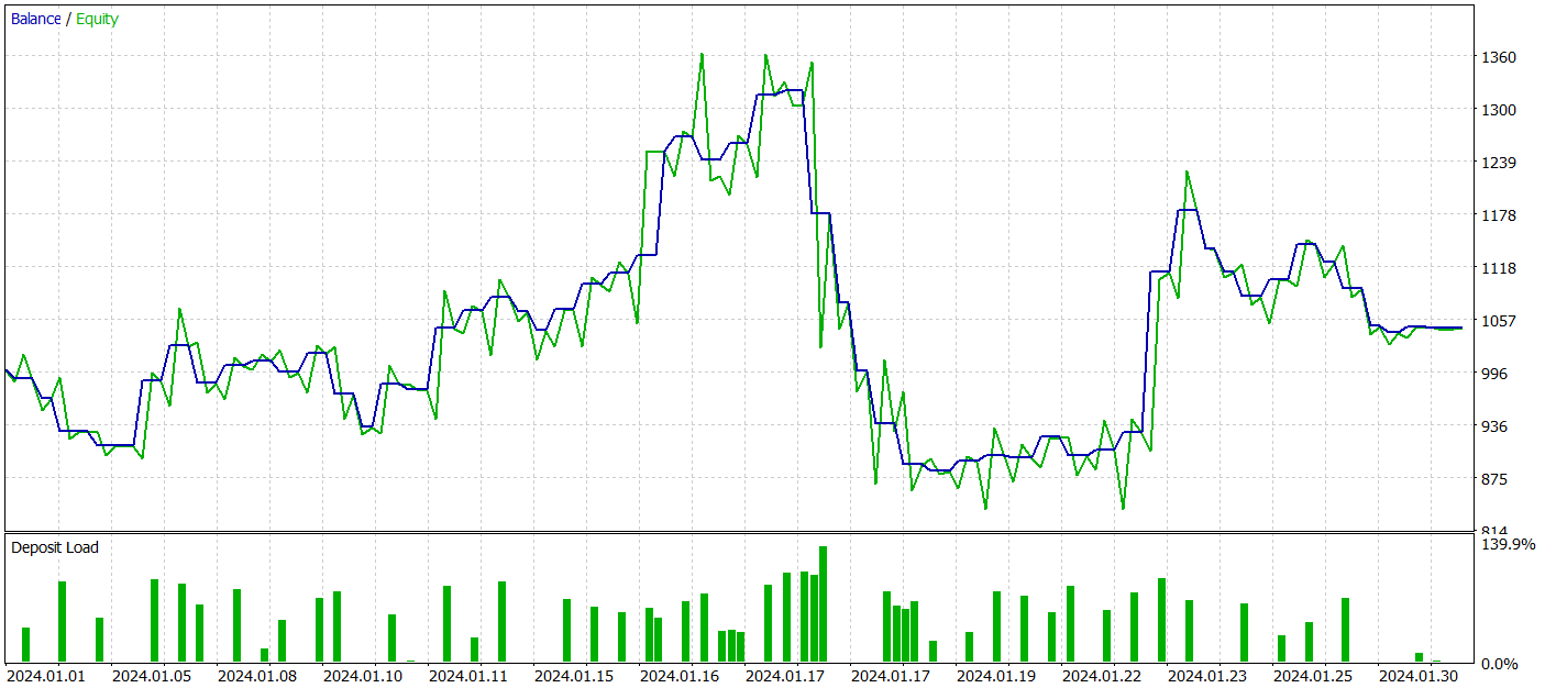
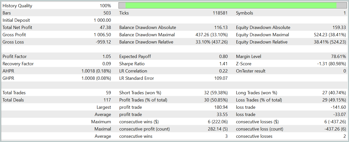
During the testing period, the model achieved a small profit. A total of 59 trades were executed, with 30 closing in profit. The maximum and average profitable trades exceeded their respective losing trades. This resulted in a profit factor of 1.05. However, the balance curve lacks a clear upward trend, and a drawdown of over 33% was recorded during testing.
Conclusion
In this article, we explored InjectTST, a novel time series forecasting method designed to enhance long-horizon predictions by injecting global information into independent data channels.
In the practical section, we implemented the proposed approaches in MQL5 and integrated them into the Environmental State Encoder model. While significant work was done, the results fell short of our expectations.
A thorough analysis is required to determine the reasons for the model's underperformance. However, one potential cause may be the direct approach taken in training the environmental state forecasting model. The authors of InjectTST originally recommended a three-stage training process, which might be necessary to achieve better results.
References
- InjectTST: A Transformer Method of Injecting Global Information into Independent Channels for Long Time Series Forecasting
- Other articles from this series
Programs used in the article
| # | Name | Type | Description |
|---|---|---|---|
| 1 | Research.mq5 | Expert Advisor | Example collection EA |
| 2 | ResearchRealORL.mq5 | Expert Advisor | EA for collecting examples using the Real-ORL method |
| 3 | Study.mq5 | Expert Advisor | Model training EA |
| 4 | StudyEncoder.mq5 | Expert Advisor | Encoder training EA |
| 5 | Test.mq5 | Expert Advisor | Model testing EA |
| 6 | Trajectory.mqh | Class library | System state description structure |
| 7 | NeuroNet.mqh | Class library | A library of classes for creating a neural network |
| 8 | NeuroNet.cl | Code Base | OpenCL program code library |
Translated from Russian by MetaQuotes Ltd.
Original article: https://www.mql5.com/ru/articles/15498
Warning: All rights to these materials are reserved by MetaQuotes Ltd. Copying or reprinting of these materials in whole or in part is prohibited.
This article was written by a user of the site and reflects their personal views. MetaQuotes Ltd is not responsible for the accuracy of the information presented, nor for any consequences resulting from the use of the solutions, strategies or recommendations described.

- Free trading apps
- Over 8,000 signals for copying
- Economic news for exploring financial markets
You agree to website policy and terms of use