Neural Networks in Trading: Practical Results of the TEMPO Method

Introduction

In the previous article we got acquainted with the theoretical aspects of the TEMPO method, which proposes an original approach to using pre-trained language models to solve time series forecasting problems. Here's a brief recall of the main innovations of the proposed algorithm.

The TEMPO method is built on the use of a pre-trained language model. In particular, the authors of the method use pre-trained GPT-2 in their experiments. The main idea of the approach lies in using the model's knowledge obtained during preliminary training to forecast time series. Here, of course, it is worth drawing non-obvious parallels between speech and the time series. Essentially, our speech is a time series of sounds that are recorded using letters. Different intonations are conveyed by punctuation marks.

The Long Language Model (LLM), such as GPT-2, was pre-trained on a large dataset (often in multiple languages) and learned a large number of different dependencies in the temporal sequence of words that we would like to use in time series forecasting. But the sequences of letters and words differ greatly from the time series data being analyzed. We have always said that for the correct operation of any model, it is very important to maintain the distribution of data in the training and test datasets. This also concerns the data analyzed during the operation of the model. Any language model does not work with the text we are accustomed to in its pure form. First, it goes through the embedding (encoding) stage, during which the text is transformed into a certain numerical code (hidden state). The model then operates on this encoded data, and at the output stage, it generates probabilities for subsequent letters and punctuation marks. The most probable symbols are then used to construct human-readable text.

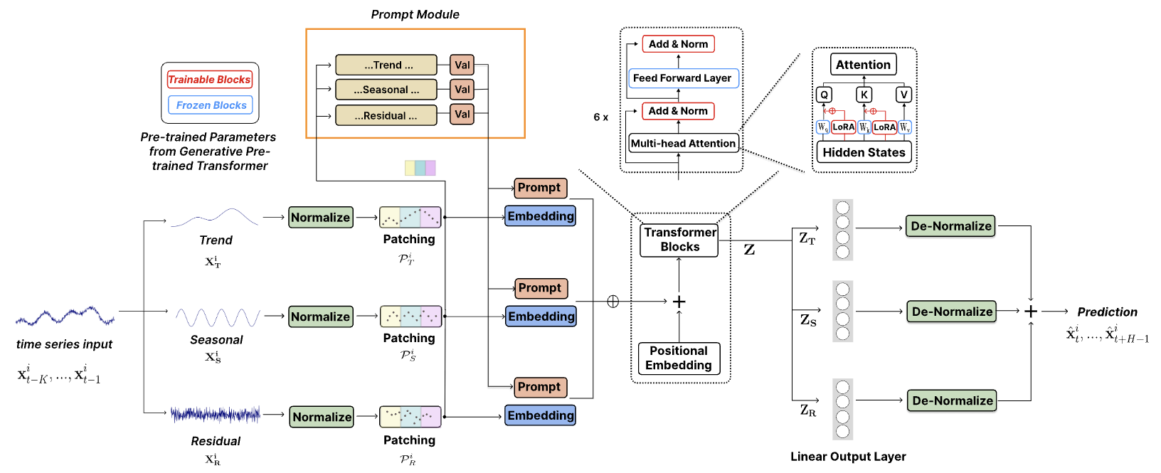
The TEMPO method takes advantage of this property. During the training process of a time series forecasting model, the parameters of the language model are "frozen," while the transformation parameters of the original data into embeddings, compatible with the model, are optimized. The authors of the TEMPO method propose a comprehensive approach to maximize the model's access to useful information. First, the analyzed time series is decomposed into its fundamental components—such as trend, seasonality, and others. Each component is then segmented and converted into embeddings that the language model can interpret. To further guide the model in the desired direction (e.g., trend or seasonality analysis), the authors introduce a system of "soft prompts".

Overall, this approach enhances model interpretability, enabling a better understanding of how different components influence the prediction of future values.

The original visualization of the method is shown below.

1. Model architecture

The proposed model architecture is quite complex, incorporating multiple branches and parallel data streams that are aggregated at the output. Implementing such an algorithm within our existing linear model framework posed significant challenges. To address this, we developed an integrated approach that encapsulates the entire algorithm within a single module, effectively functioning as a single-layer implementation. While this approach somewhat limits users' ability to experiment with varying model complexities - since the structural flexibility of the module is constrained by the parameters of the Init method in our CNeuronTEMPOOCL class - it also significantly simplifies the process of building new models. Users are not required to delve into the intricate details of the architecture. Instead, they only need to specify a few key parameters to construct a robust and sophisticated model architecture. In our view, this trade-off is more practical for the majority of users.

Additionally, one crucial aspect to consider is that the authors of the TEMPO method conducted their experiments using a pre-trained GPT-2 language model. When implementing this in Python, such models can be accessed via libraries like Hugging Face. However, in our implementation, we do not use a pre-trained language model. Instead, we replace it with a cross-attention block, which will be trained alongside the main model.

The TEMPO method is positioned as a time series forecasting model. Consequently, as with similar cases, we integrate its proposed techniques into our Environmental State Encoder model. The architecture of this model is defined in the CreateEncoderDescriptions method.

Within the parameters of this method, we pass a pointer to a dynamic array, where the architectural parameters of the neural layers in the generated model will be stored.

bool CreateEncoderDescriptions(CArrayObj *&encoder)
  {
//---
   CLayerDescription *descr;
//---
   if(!encoder)
     {
      encoder = new CArrayObj();
      if(!encoder)
         return false;
     }

In the method body, we check the relevance of the received pointer and, if necessary, create a new instance of the object.

This is followed by a description of the model. First, we specify a fully connected layer for recording the input data. The size of the created layer must match the size of the input data tensor.

//--- Encoder
   encoder.Clear();
//--- Input layer
   if(!(descr = new CLayerDescription()))
      return false;
   descr.type = defNeuronBaseOCL;
   int prev_count = descr.count = (HistoryBars * BarDescr);
   descr.activation = None;
   descr.optimization = ADAM;
   if(!encoder.Add(descr))
     {
      delete descr;
      return false;
     }

As a reminder, the model receives a tensor of raw input data in its original form, exactly as obtained from the terminal. In all our previous models, the next step involved applying a batch normalization layer to perform preliminary data processing and bring the values to a comparable scale.

However, in this case, we have deliberately excluded the batch normalization layer. Surprisingly, this decision stems from the architecture of the TEMPO method itself. As illustrated in the visualization above, the raw data is immediately directed to the decomposition block, where the analyzed time series is broken down into its three fundamental components: trend, seasonality, and residuals. This decomposition occurs independently for each univariate time series - i.e., for each analyzed parameter of the multimodal time series. The comparability of values within each univariate series is inherently ensured by the nature of the data.

First, the trend component is extracted from the raw data. In our implementation, we achieve this using a piecewise-linear representation of the time series. As you are aware, this method’s algorithm enables the extraction of comparable segments regardless of the scaling and shifting of the raw data distribution that would typically occur during normalization.

Next, we subtract the trend component from the original data and determine the seasonal component. This is accomplished using the discrete Fourier transform, which decomposes the signal into its frequency spectrum, allowing us to identify the most significant periodic dependencies based on amplitude. Like trend extraction, frequency decomposition is also insensitive to data scaling and shifting.

Finally, the residual component is obtained by subtracting the two previously extracted components from the original data.

At this point, it becomes evident that from a model design perspective, preliminary data normalization offers no additional benefits. Moreover, applying normalization at this stage would introduce extra computational overhead, which is undesirable in itself.

Now, consider the next stage. The authors of the TEMPO method introduce normalization of the extracted components, which is clearly essential for subsequent operations with multimodal data. This raises a question: Could we modify the normalization approach? Specifically, could we normalize the raw input data before decomposition and then omit normalization for the individual components? After all, the raw data volume is three times smaller than the combined size of the extracted components. In my view, the answer is likely "no".

To illustrate, let’s take an abstract time series graph and highlight its key trends. It is evident that the trend component encapsulates the majority of the information.

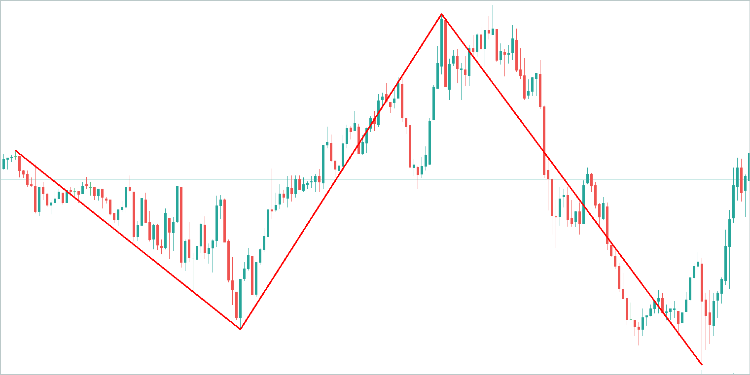
The seasonal component consists of wave-like fluctuations around the trend line, with significantly lower amplitude than the trend itself.

The residual component, representing other variations, has even lower amplitude, primarily reflecting noise. However, this noise cannot be ignored, as it captures external influences such as news events and other unaccounted-for factors that exhibit a non-systematic nature.

Normalizing the raw data before decomposition would address the issue of comparability among individual univariate series. However, it would not solve the problem of comparability between the extracted components themselves. For model stability, it is therefore preferable to apply normalization at the component level after decomposition.

Based on this reasoning, we exclude the batch normalization layer for raw input data. Instead, we introduce our new TEMPO method block immediately after the input data layer.

//--- layer 1
   if(!(descr = new CLayerDescription()))
      return false;
   descr.type = defNeuronTEMPOOCL;
   descr.count = HistoryBars;
   descr.window = BarDescr;
   descr.step = NForecast;

We specify the size of the analyzed multimodal sequence, the number of unitary time series in it, and the planning horizon using previously specified constants.

As part of the experiment in preparing this article, I specified 4 attention heads.

   descr.window_out = 4;

I also set 4 nested layers in the attention block.

   descr.layers = 4;

Here I want to remind you that these parameters are used in 2 nested attention blocks:

• frequency domain attention block used to identify dependencies between the frequency characteristics of individual unitary sequences, and
• cross-attention block for detecting dependencies in a sequence of time series.

Next, we specify the normalization batch size and the model optimization method.

   descr.batch = 1e4;
   descr.activation = None;
   descr.optimization = ADAM;
   if(!encoder.Add(descr))
     {
      delete descr;
      return false;
     }

At this point the model could be considered complete, since at the output of the CNeuronTEMPOOCL block we get the desired forecast values of the analyzed time series. But we will add the final touch - a frequency matching layer for the forecast time series, CNeuronFreDFOCL.

//--- layer 2
   if(!(descr = new CLayerDescription()))
      return false;
   descr.type = defNeuronFreDFOCL;
   descr.window = BarDescr;
   descr.count =  NForecast;
   descr.step = int(true);
   descr.probability = 0.7f;
   descr.activation = None;
   descr.optimization = ADAM;
   if(!encoder.Add(descr))
     {
      delete descr;
      return false;
     }
//---
   return true;
  }

As a result, we get a short and concise model architecture in the form of 3 neural layers. However, underneath it lies a complex, integrated algorithm. After all, we know what's under the "tip of the iceberg", CNeuronTEMPOOCL, 24 nested layers are hidden, 12 of which contain trainable parameters. Moreover, 2 of these nested layers are attention units, for which we specified the creation of a four-layer Self-Attention architecture with 4 attention heads in each. This makes our model truly complex and deep.

We will use the obtained forecast values of the upcoming price movement to train the Actor's behavior policy. Here we have largely retained the architectures from the previous articles, but due to the complexity of the Environment State Encoder and the expected increase in the cost of training it, I decided to reduce the number of nested layers in the cross-attention blocks of the Actor and Critic models. As a reminder, the description of the architecture of these models is presented in the CreateDescriptions method, in the parameters of which we pass pointers to 2 dynamic arrays. So, we will write the description of the architecture of our models into these arrays.

bool CreateDescriptions(CArrayObj *&actor, CArrayObj *&critic)
  {
//---
   CLayerDescription *descr;
//---
   if(!actor)
     {
      actor = new CArrayObj();
      if(!actor)
         return false;
     }
   if(!critic)
     {
      critic = new CArrayObj();
      if(!critic)
         return false;
     }

In the body of the method, we check the relevance of the received pointers and, if necessary, create new instances of objects.

First we describe the Actor architecture, to which we input the tensor describing the state of the account.

//--- Actor
   actor.Clear();
//--- Input layer
   if(!(descr = new CLayerDescription()))
      return false;
   descr.type = defNeuronBaseOCL;
   int prev_count = descr.count = AccountDescr;
   descr.activation = None;
   descr.optimization = ADAM;
   if(!actor.Add(descr))
     {
      delete descr;
      return false;
     }

Please note that here we are talking about the state of the account, not the environment. By the term "state of environment" we mean the parameters of price movement dynamics and analyzed indicators. In "state of the account" we include the current value of the account balance, the volume and direction of open positions, as well as the profit or loss accumulated on them.

We transform the information received at the input of the model into a hidden state using a basic fully connected layer.

//--- layer 1
   if(!(descr = new CLayerDescription()))
      return false;
   descr.type = defNeuronBaseOCL;
   prev_count = descr.count = EmbeddingSize;
   descr.activation = SIGMOID;
   descr.optimization = ADAM;
   if(!actor.Add(descr))
     {
      delete descr;
      return false;
     }

Next we use a cross-attention block where we compare the current account state with the predicted value of the upcoming price movement obtained from the Environment State Encoder.

//--- layer 2
   if(!(descr = new CLayerDescription()))
      return false;
   descr.type = defNeuronMLCrossAttentionMLKV;
     {
      int temp[] = {1, NForecast};
      ArrayCopy(descr.units, temp);
     }
     {
      int temp[] = {EmbeddingSize, BarDescr};
      ArrayCopy(descr.windows, temp);
     }
     {
      int temp[] = {4, 2};
      ArrayCopy(descr.heads, temp);
     }
   descr.layers = 4;
   descr.step = 1;
   descr.window_out = 32;
   descr.activation = None;
   descr.optimization = ADAM;
   if(!actor.Add(descr))
     {
      delete descr;
      return false;
     }

Here, it is important to focus on one key aspect - the subspace of data values obtained from the State Score Encoder. While we previously employed the same approach, it did not raise any concerns at the time. So, what has changed?

As they say, "the devil is in the details". Previously, we used a batch normalization layer at the input of the Environmental State Encoder to bring raw data into a comparable format. At the model's output, we applied the CNeuronRevINDenormOCL layer to reverse this transformation, restoring the data to its original subspace. For the Actor and Critic, we worked with the hidden representation of predictive values in a comparable form before applying shift and scaling operations back into the original data subspaces. This ensured that subsequent analysis relied on consistent and interpretable data, making it easier for the model to process.

However, in the case of CNeuronTEMPOOCL, we deliberately omitted the preliminary normalization of input data, as previously discussed. As a result, the model now outputs unnormalized predicted price movements, which may complicate the tasks of the Actor and Critic and, consequently, reduce their effectiveness. One potential solution is to normalize the predicted time series values before their subsequent use. The simplest way to achieve this would be to introduce a small preprocessing model with a single normalization layer. However, we did not implement this step.

Additionally, I would like to remind you that instead of simply summing the three forecast components (trend, seasonality, and others) at the output of the CNeuronTEMPOOCL block, we used a convolutional layer without an activation function. This replaces simple summation with a weighted summation of the obtained data.

   if(!cSum.Init(0, 24, OpenCL, 3, 3, 1, iVariables, iForecast, optimization, iBatch))
      return false;
   cSum.SetActivationFunction(None);

Limiting the maximum value of the model parameters to less than 1 allows us to exclude obviously large values at the model output.

#define MAX_WEIGHT 1.0e-3f

Of course, this approach inherently limits the accuracy of our Environmental State Encoder. After all, how can we align real indicator values, such as RSI (which ranges from 0 to 100), with predicted results whose absolute values are below 1? In such cases, when using MSE as the loss function, there is a high likelihood that the predicted values will reach the maximum possible level. To address this, we introduced the CNeuronFreDFOCL frequency alignment block at the output of the Environmental State Encoder. This block is less sensitive to data scaling and enables the model to learn the structure of upcoming price movements, which, in this context, is more important than absolute values.

I acknowledge that this proposed solution is not immediately intuitive and may be somewhat challenging to grasp. However, its effectiveness will ultimately be evaluated based on the practical results of our models.

Now, returning to the architecture of our Actor: following the cross-attention block, we employ a perceptron composed of three fully connected layers for decision-making.

//--- layer 3
   if(!(descr = new CLayerDescription()))
      return false;
   descr.type = defNeuronBaseOCL;
   descr.count = LatentCount;
   descr.activation = SIGMOID;
   descr.optimization = ADAM;
   if(!actor.Add(descr))
     {
      delete descr;
      return false;
     }
//--- layer 4
   if(!(descr = new CLayerDescription()))
      return false;
   descr.type = defNeuronBaseOCL;
   descr.count = LatentCount;
   descr.activation = SIGMOID;
   descr.optimization = ADAM;
   if(!actor.Add(descr))
     {
      delete descr;
      return false;
     }
//--- layer 5
   if(!(descr = new CLayerDescription()))
      return false;
   descr.type = defNeuronBaseOCL;
   descr.count = 2 * NActions;
   descr.activation = None;
   descr.optimization = ADAM;
   if(!actor.Add(descr))
     {
      delete descr;
      return false;
     }

At its output we add stochasticity to the policy of our Actor.

//--- layer 6
   if(!(descr = new CLayerDescription()))
      return false;
   descr.type = defNeuronVAEOCL;
   descr.count = NActions;
   descr.optimization = ADAM;
   if(!actor.Add(descr))
     {
      delete descr;
      return false;
     }

We then align the frequency characteristics of the adopted solution.

//--- layer 7
   if(!(descr = new CLayerDescription()))
      return false;
   descr.type = defNeuronFreDFOCL;
   descr.window = NActions;
   descr.count =  1;
   descr.step = int(false);
   descr.probability = 0.7f;
   descr.activation = None;
   descr.optimization = ADAM;
   if(!actor.Add(descr))
     {
      delete descr;
      return false;
     }

The architecture of the Critic almost completely repeats the Actor architecture presented above. There are only minor differences. In particular, we feed the model's input not with the account state, but with the Actor's action tensor.

//--- Critic
   critic.Clear();
//--- Input layer
   if(!(descr = new CLayerDescription()))
      return false;
   descr.type = defNeuronBaseOCL;
   prev_count = descr.count = NActions;
   descr.activation = None;
   descr.optimization = ADAM;
   if(!critic.Add(descr))
     {
      delete descr;
      return false;
     }

At the output of the model we do not use stochasticity, giving a clear assessment of the proposed actions.

//--- layer 6
   if(!(descr = new CLayerDescription()))
      return false;
   descr.type = defNeuronBaseOCL;
   descr.count = NRewards;
   descr.activation = None;
   descr.optimization = ADAM;
   if(!critic.Add(descr))
     {
      delete descr;
      return false;
     }
//--- layer 7
   if(!(descr = new CLayerDescription()))
      return false;
   descr.type = defNeuronFreDFOCL;
   descr.window = NRewards;
   descr.count =  1;
   descr.step = int(false);
   descr.probability = 0.7f;
   descr.activation = None;
   descr.optimization = ADAM;
   if(!critic.Add(descr))
     {
      delete descr;
      return false;
     }
//---
   return true;
  }

You can find a full description of the architectural solutions of all the models used in the attachment.

2. Model Training

As observed from the architectural description of the trained models above, the implementation of the TEMPO method has not altered the structure of the original data or the results of the trained models. Therefore, we can confidently use previously collected training datasets for the initial model training. Furthermore, we can continue collecting data, training models, and updating the training dataset using the previously developed programs for environment interaction and model training.

For interacting with the environment and gathering training data, we use two programs:

• "...\Experts\TEMPO\ResearchRealORL.mq5" — collects data based on a historical set of real trades. The methodology is detailed in the referenced article.
• "...\Experts\TEMPO\Research.mq5" — Expert Advisor primarily designed to analyze the performance of a pre-trained policy and update the training dataset within the current policy environment. This enables fine-tuning of the Actor's policy based on real reward feedback. However, this EA can also be used to collect an initial training dataset based on the Actor's behavior policy initialized with random parameters.

Regardless of whether we already have collected environment interaction data, we can launch any of the above expert advisors in the MetaTrader 5 strategy tester to create a new training dataset or update an existing one.

The collected training data is first used to train the Environmental State Encoder to predict future price movements. For this, we run the "...\Experts\TEMPO\StudyEncoder.mq5" EA in real-time mode in MetaTrader 5.

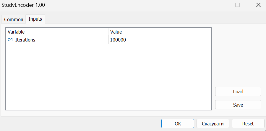
It is important to note that during training, the Environmental State Encoder operates solely on price dynamics and analyzed indicators, which are not influenced by the Agent's actions. Therefore, all training dataset passes on the same historical segment remain identical for the model. Consequently, updating the training dataset during encoder training does not provide additional information. Thus, we must be patient and train the model until we achieve satisfactory results.

Once again, I would like to emphasize that due to the specifics of our architectural approach, as discussed earlier, we do not expect "low" error values at this stage. However, we still aim to minimize the error as much as possible, stopping the training process when the prediction error stabilizes within a narrow range.

The second stage involves iterative training of the Actor and Critic models. At this stage, we use the "...\Experts\TEMPO\Study.mq5" EA, which is also run in real-time mode. This time, we "freeze" the Environmental State Encoder parameters and train the two models (Actor and Critic) in parallel.

The Critic learns the environment's reward function from the training dataset, mapping the predicted environment state and the Agent’s actions from the training dataset to estimate the expected reward. This stage follows supervised learning principles, as the actual rewards for the executed actions are stored in the training dataset.

The Actor then optimizes its policy based on feedback from the Critic, aiming to maximize overall profitability.

This process is iterative, as the Actor's action subspace shifts during training. To maintain relevance, we need to update the training dataset to capture real rewards in the newly adjusted action subspace. This allows the Critic to refine the reward function and provide a more accurate assessment of the Actor's actions, thereby guiding policy adjustments in the desired direction.

To update the training dataset, we re-run the slow optimization process of the "...\Experts\TEMPO\Research.mq5" EA.

At this stage, one might question the necessity of training the State Score Encoder separately from the other models. On the one hand, a pre-trained State Score Encoder provides the most probable market movements, effectively acting as a digital filter that reduces noise in the raw data. Additionally, we use a planning horizon significantly shorter than the depth of the analyzed history. This means the Encoder also compresses data for subsequent analysis, potentially improving the efficiency of the Actor and Critic models.

On the other hand, do we truly need a forecast of future price movements? We have previously emphasized that what matters more is a clear interpretation of the current state, allowing the Agent to select the optimal action with maximum accuracy. To explore this question, we developed another training EA: "...\Experts\TEMPO\Study2.mq5". This program is based on "...\Experts\TEMPO\Study.mq5". Therefore, we will focus solely on its direct model training method: Train.

void Train(void)
  {
//---
   vector<float> probability = GetProbTrajectories(Buffer, 0.9);
//---
   vector<float> result, target, state;
   bool Stop = false;

In the body of the method, we first generate a vector of probabilities of choosing trajectories from the experience replay buffer based on the total profitability of the passes. After that we initialize the necessary local variables.

At this point we complete the preparatory work and organize the model training loop.

   for(int iter = 0; (iter < Iterations && !IsStopped() && !Stop); iter ++)
     {
      int tr = SampleTrajectory(probability);
      int i = (int)((MathRand() * MathRand() / MathPow(32767, 2)) * (Buffer[tr].Total - 2 - NForecast));
      if(i <= 0)
        {
         iter --;
         continue;
        }
      state.Assign(Buffer[tr].States[i].state);
      if(MathAbs(state).Sum() == 0)
        {
         iter --;
         continue;
        }

In the loop body, we sample one trajectory from the experience replay buffer and randomly select an environment state on it.

We transfer the description of the selected environmental state from the training sample to the data buffer and perform a feed-forward pass of the Environmental State Encoder.

      bState.AssignArray(state);
      //--- State Encoder
      if(!Encoder.feedForward((CBufferFloat*)GetPointer(bState), 1, false, (CBufferFloat*)NULL))
        {
         PrintFormat("%s -> %d", __FUNCTION__, __LINE__);
         Stop = true;
         break;
        }

Then we take from the experience replay buffer the Agent's actions performed in the selected state when interacting with the environment, and perform their assessment by the Critic.

      //--- Critic
      bActions.AssignArray(Buffer[tr].States[i].action);
      if(bActions.GetIndex() >= 0)
         bActions.BufferWrite();
      Critic.TrainMode(true);
      if(!Critic.feedForward((CBufferFloat*)GetPointer(bActions), 1, false, GetPointer(Encoder), LatentLayer))
        {
         PrintFormat("%s -> %d", __FUNCTION__, __LINE__);
         Stop = true;
         break;
        }

Note that the experience replay buffer contains the actual evaluation of these actions and we can adjust the reward function learned by the Critic towards minimizing errors. To do this, we extract the actual reward received from the experience replay buffer and perform Critic's backpropagation pass.

      result.Assign(Buffer[tr].States[i + 1].rewards);
      target.Assign(Buffer[tr].States[i + 2].rewards);
      result = result - target * DiscFactor;
      Result.AssignArray(result);
      if(!Critic.backProp(Result, (CNet *)GetPointer(Encoder), LatentLayer) ||
         !Encoder.backPropGradient((CBufferFloat*)NULL))
        {
         PrintFormat("%s -> %d", __FUNCTION__, __LINE__);
         Stop = true;
         break;
        }

In this step, we add a backpropagation pass of the Environment State Encoder to draw the model's attention to reference points, allowing for more accurate action estimates.

The next step is to adjust the Actor's policy. First, from the experience replay buffer, we prepare a description of the account state corresponding to the previously selected state of the environment.

      //--- Policy
      float PrevBalance = Buffer[tr].States[MathMax(i - 1, 0)].account[0];
      float PrevEquity = Buffer[tr].States[MathMax(i - 1, 0)].account[1];
      bAccount.Clear();
      bAccount.Add((Buffer[tr].States[i].account[0] - PrevBalance) / PrevBalance);
      bAccount.Add(Buffer[tr].States[i].account[1] / PrevBalance);
      bAccount.Add((Buffer[tr].States[i].account[1] - PrevEquity) / PrevEquity);
      bAccount.Add(Buffer[tr].States[i].account[2]);
      bAccount.Add(Buffer[tr].States[i].account[3]);
      bAccount.Add(Buffer[tr].States[i].account[4] / PrevBalance);
      bAccount.Add(Buffer[tr].States[i].account[5] / PrevBalance);
      bAccount.Add(Buffer[tr].States[i].account[6] / PrevBalance);
      double time = (double)Buffer[tr].States[i].account[7];
      double x = time / (double)(D'2024.01.01' - D'2023.01.01');
      bAccount.Add((float)MathSin(x != 0 ? 2.0 * M_PI * x : 0));
      x = time / (double)PeriodSeconds(PERIOD_MN1);
      bAccount.Add((float)MathCos(x != 0 ? 2.0 * M_PI * x : 0));
      x = time / (double)PeriodSeconds(PERIOD_W1);
      bAccount.Add((float)MathSin(x != 0 ? 2.0 * M_PI * x : 0));
      x = time / (double)PeriodSeconds(PERIOD_D1);
      bAccount.Add((float)MathSin(x != 0 ? 2.0 * M_PI * x : 0));
      if(bAccount.GetIndex() >= 0)
         bAccount.BufferWrite();

We run the Actor's feed-forward pass to generate an action vector taking into account the current policy.

      //--- Actor
      if(!Actor.feedForward((CBufferFloat*)GetPointer(bAccount), 1, false, GetPointer(Encoder), LatentLayer))
        {
         PrintFormat("%s -> %d", __FUNCTION__, __LINE__);
         Stop = true;
         break;
        }

After that, we disable the training mode for the Critic and evaluate the actions generated by the Actor.

      Critic.TrainMode(false);
      if(!Critic.feedForward((CNet *)GetPointer(Actor), -1, (CNet*)GetPointer(Encoder), LatentLayer))
        {
         PrintFormat("%s -> %d", __FUNCTION__, __LINE__);
         Stop = true;
         break;
        }

We adjust the Actor's policy in 2 stages. First, we check the effectiveness of the current pass. If, in the process of interaction with the environment, this pass turned out to be profitable, then we will adjust the Actor's action policy towards the actions stored in the experience replay buffer.

      if(Buffer[tr].States[0].rewards[0] > 0)
         if(!Actor.backProp(GetPointer(bActions), GetPointer(Encoder), LatentLayer) ||
            !Encoder.backPropGradient((CBufferFloat*)NULL))
           {
            PrintFormat("%s -> %d", __FUNCTION__, __LINE__);
            Stop = true;
            break;
           }

At the same time, we also adjust the Environmental State Encoder parameters to identify data points that influence Actor's policy effectiveness.

In the second stage of the Actor policy training we will offer Critic to indicate the direction of adjustment of the agent's actions to increase profitability/reduce unprofitability by 1%. To do this, we take the current rating of the Actor's actions and improve it by 1%.

      Critic.getResults(Result);
      for(int c = 0; c < Result.Total(); c++)
        {
         float value = Result.At(c);
         if(value >= 0)
            Result.Update(c, value * 1.01f);
         else
            Result.Update(c, value * 0.99f);
        }

We use the obtained result as a reference for the Critic's backpropagation pass. As a reminder, at this stage we have disabled the Critic's learning process. Therefore, when performing a backpropagation pass, its parameters will not be adjusted. But the Actor will receive an error gradient. And we will be able to adjust the Actor’s parameters towards increasing the effectiveness of its policy.

      if(!Critic.backProp(Result, (CNet *)GetPointer(Encoder), LatentLayer) ||
         !Actor.backPropGradient((CNet *)GetPointer(Encoder), LatentLayer, -1, true) ||
         !Encoder.backPropGradient((CBufferFloat*)NULL))
        {
         PrintFormat("%s -> %d", __FUNCTION__, __LINE__);
         Stop = true;
         break;
        }

Next, we just need to inform the user about the model training progress and move on to the next iteration of the loop.

      if(GetTickCount() - ticks > 500)
        {
         double percent = double(iter + i) * 100.0 / (Iterations);
         string str = StringFormat("%-14s %6.2f%% -> Error %15.8f\n", "Actor", percent, Actor.getRecentAverageError());
         str += StringFormat("%-14s %6.2f%% -> Error %15.8f\n", "Critic", percent, Critic.getRecentAverageError());
         Comment(str);
         ticks = GetTickCount();
        }
     }

Once the training process is complete, we clear the comments field on the symbol chart.

   Comment("");
//---
   PrintFormat("%s -> %d -> %-15s %10.7f", __FUNCTION__, __LINE__, "Actor", Actor.getRecentAverageError());
   PrintFormat("%s -> %d -> %-15s %10.7f", __FUNCTION__, __LINE__, "Critic", Critic.getRecentAverageError());
   ExpertRemove();
//---
  }

We output the model training results to the terminal log and initialize the EA termination process.

The complete code for this Expert Advisor, along with all the programs used in the preparation of this article, is available in the attachment.

3. Testing

After completing the development and training phases, we have reached the key stage: the practical evaluation of our trained models.

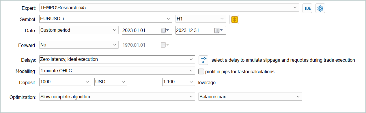
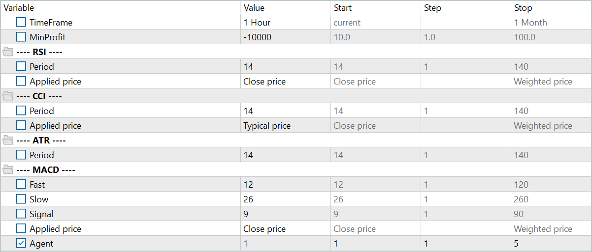
The models were trained on historical data for the EURUSD instrument over the entire year of 2023 on the H1 timeframe. All indicator parameters were set to their default values.

Testing of the trained models was conducted on historical data from January 2024 while keeping all other parameters unchanged. This approach ensures the closest possible approximation to real-world operating conditions.

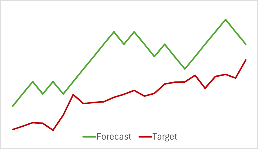
At the first stage, we trained the Environmental State Encoder model. Below is a visualization of the actual and predicted price movements over a 24-hour period with a forecast step of one hour, corresponding to the following day on the H1 timeframe. The same timeframe was used for analysis. 

From the presented chart, we can observe that the generated forecast generally captured the main direction of the upcoming movement. It even managed to align in both timing and direction with certain local extrema. However, the predicted price trajectory appears smoother, resembling trendlines drawn over the instrument's price chart.

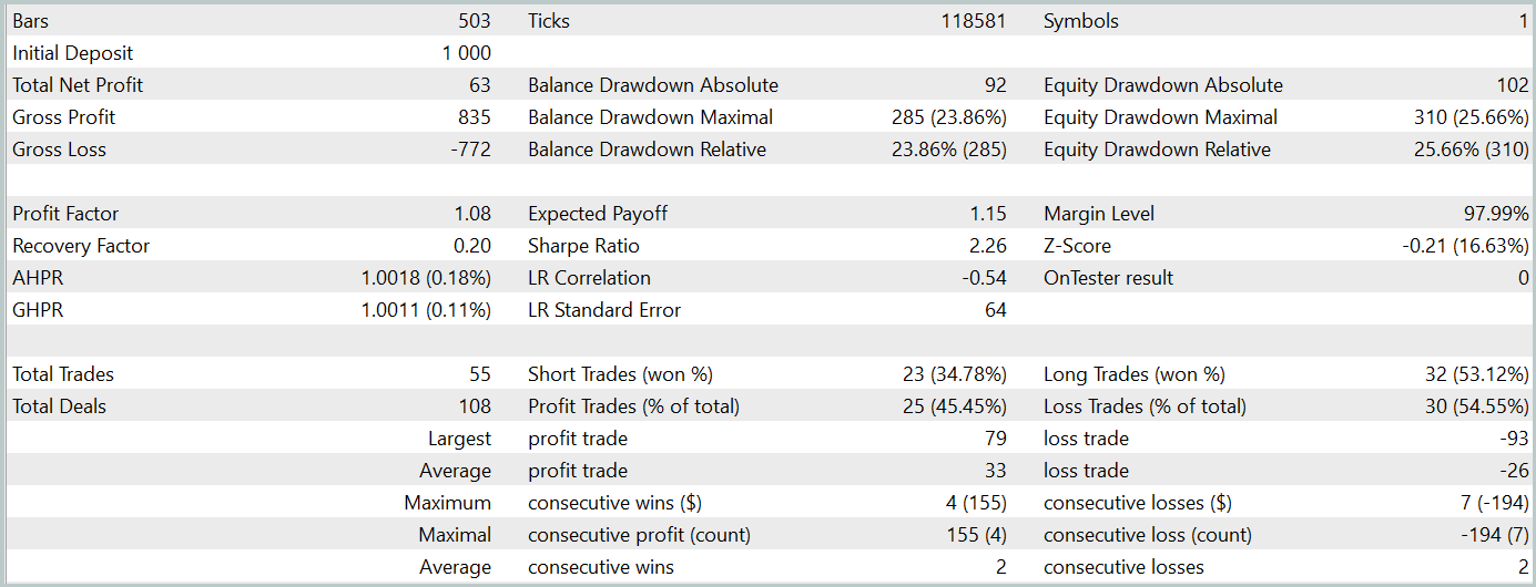
In the second stage, we trained the Actor and Critic models. We will not evaluate the accuracy of Critic's assessment of actions. Because its main task is to direct the Actor policy training in the right direction. Instead, we focus on the profitability of the Actor's learned policy during the test period. The Actor's performance in the strategy tester is presented below.  

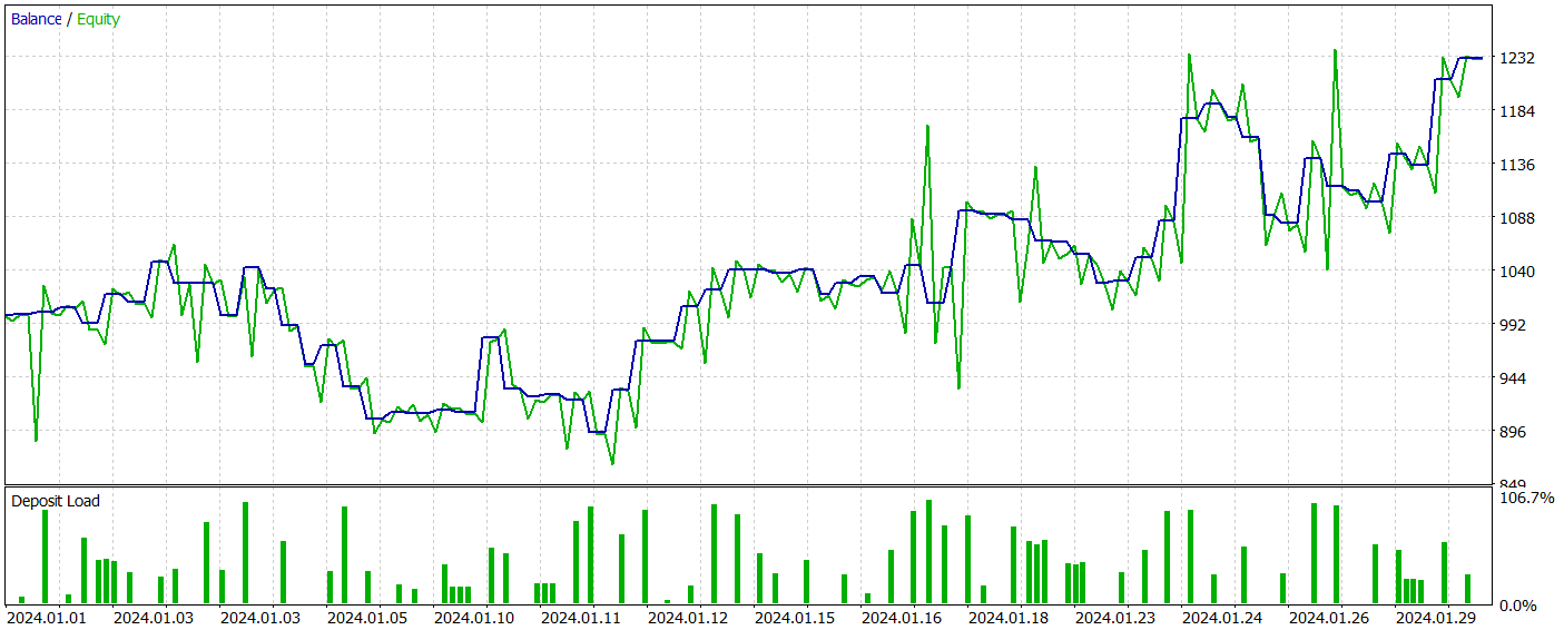
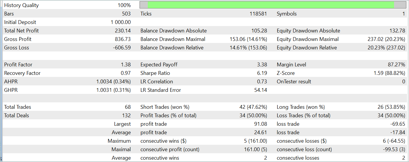
During the test period (January 2024), the Actor executed 68 trades, with half of them closing in profit. More importantly, both the maximum and average profitable trades exceeded their losing counterparts (91.08 and 24.61 vs. -69.85 and -17.84, respectively), resulting in an overall profit of 23%.

However, the equity chart reveals significant fluctuations above and below the balance line. This initially raises concerns about "holding onto losses" and delayed position exits. Notably, at these moments, the deposit load approaches 100%, suggesting excessive risk exposure. This is further confirmed by the maximum drawdown exceeding 20%.

Next, we performed additional training of the Actor's policy with adjustments to the Environmental State Encoder's parameters. It is important to highlight that this fine-tuning was done without updating the training dataset. In other words, the training base remained unchanged. However, this process had a negative effect. Model performance deteriorated: the number of trades decreased, the percentage of profitable trades dropped to 45%, overall profitability declined, and the equity drawdown exceeded 25%.

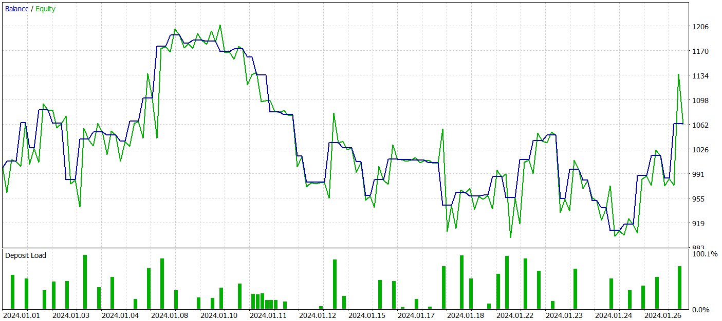
Interestingly, the accuracy of predicted price movement trajectories also changed.

My perspective is that when we begin optimizing the Environmental State Encoder's parameters to align with the goals of the Actor and Critic, we introduce additional noise at the Encoder's output. During the initial training phase, the predictive model had a clear correspondence between input data and results, allowing it to learn and generalize patterns effectively. However, the error gradient received from the Actor and Critic introduces conflicting noise as the model attempts to minimize its error based on the data provided by the Environmental State Encoder. As a result, the Encoder ceases to function as a filter for raw data, leading to reduced effectiveness across all models.

Conclusion

We explored an innovative and complex method for time series forecasting, TEMPO, in which the authors proposed using pre-trained language models for time series prediction tasks. The proposed algorithm introduces a novel approach to time series decomposition, improving the efficiency of learning data representations.

We conducted extensive work implementing these approaches in MQL5. Despite not having access to a pre-trained language model, our experiments yielded intriguing results.

Overall, the proposed methods can be applied to the development of real trading models. However, it is essential to recognize that training models based on Transformer architectures requires the collection of substantial amounts of data and can be computationally expensive.

References

• TEMPO: Prompt-based Generative Pre-trained Transformer for Time Series Forecasting
• Other articles from this series

Programs used in the article

#	Name	Type	Description
1	Research.mq5	Expert Advisor	Example collection EA
2	ResearchRealORL.mq5	Expert Advisor	EA for collecting examples using the Real-ORL method
3	Study.mq5	Expert Advisor	Model training EA
4	StudyEncoder.mq5	Expert Advisor	Encoder training EA
5	Test.mq5	Expert Advisor	Model testing EA
6	Trajectory.mqh	Class library	System state description structure
7	NeuroNet.mqh	Class library	A library of classes for creating a neural network
8	NeuroNet.cl	Code Base	OpenCL program code library
9	Study2.mq5	Expert Advisor	Expert Advisor for training Actor and Critic models with Encoder parameter adjustments