
Neural Networks in Trading: Using Language Models for Time Series Forecasting

Introduction
Throughout this series of articles, we have explored a variety of architectural approaches for time series modeling. Many of these approaches achieve commendable results. However, it is evident that they do not fully use the advantage of complex patterns present in time series, such as seasonality and trend. These components are fundamental distinguishing characteristics of time series data. Consequently, recent studies suggest that deep learning-based architectures may not be as robust as previously believed, with even shallow neural networks or linear models outperforming them on certain benchmarks.
Meanwhile, the emergence of basic models in natural language processing (NLP) and computer vision (CV) has marked significant milestones in effective representation learning. Pretraining foundational models for time series using large datasets enhances performance in subsequent tasks. Moreover, large language models enable the use of pre-trained representations instead of requiring models to be trained from scratch. However, existing foundational structures and methodologies in language models do not fully capture the evolution of temporal patterns, which is crucial for time series modeling.
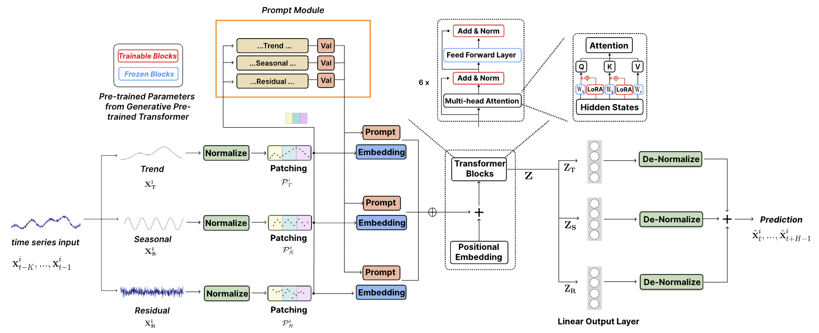
The authors of the paper "TEMPO: Prompt-based Generative Pre-trained Transformer for Time Series Forecasting" address the critical challenge of adapting large pre-trained models for time series forecasting. They propose TEMPO, a comprehensive model based on GPT, designed for effective time series representation learning. TEMPO consists of two key analytical components: one focusing on modeling specific time series patterns such as trends and seasonality, and the other aimed at deriving more generalized insights from intrinsic data properties through a prompt-based approach. Specifically, TEMPO first decomposes the original multimodal time series data into three components: trend, seasonality, and residuals. Each component is then mapped into a corresponding latent space to construct the initial time series embedding for GPT.
The authors conduct a formal analysis linking the time series domain with the frequency domain to emphasize the necessity of decomposing such components for time series analysis. They also theoretically demonstrate that the attention mechanism struggles to perform this decomposition automatically.
TEMPO uses prompts that encode temporal knowledge about trends and seasonality, effectively fine-tuning GPT for forecasting tasks. Additionally, trend, seasonality, and residuals are used to provide an interpretable structure for understanding the interactions between the original components.
1. The TEMPO Algorithm
In their work, the authors of TEMPO adopt a hybrid approach that combines the robustness of statistical time series analysis with the adaptability of data-driven methods. They introduce a novel integration of seasonal and trend decomposition into pre-trained language models based on the Transformer architecture. This strategy harnesses the unique advantages of both statistical and machine learning methods, enhancing the model's ability to process time series data efficiently.
Additionally, they introduce a semi-soft prompt-based approach, increasing the adaptability of pre-trained models for time series processing. This innovative technique enables models to integrate their extensive pre-trained knowledge with the specific requirements of time series analysis.
For multimodal time series data, decomposing complex raw data into meaningful components such as trends and seasonality helps optimize information extraction.
![]()
Trend Component XT captures long-term patterns in the data. Seasonal Component XS encapsulates repetitive short-term cycles, assessed after removing the trend. Residual Component XR represents the remaining part of the data after extracting trend and seasonality.
In practice, utilizing as much information as possible is recommended for more accurate decomposition. However, to maintain computational efficiency, the authors opt for a localized decomposition using a fixed-size window rather than a global decomposition over the entire dataset. Trainable parameters are introduced to estimate various components of local decomposition, extending this principle to other model components.
Experimental results demonstrate that decomposition significantly simplifies the forecasting process.
The proposed decomposition of raw data is crucial for modern Transformer-based architectures since attention mechanisms theoretically cannot automatically disentangle unidirectional trend and seasonal signals. If trend and seasonal components are non-orthogonal, they cannot be completely separated using any set of orthogonal bases. The Self-Attention layer naturally transforms into an orthogonal transformation, similar to Principal Component Analysis. Thus, directly attending to raw time series data would be ineffective for disentangling non-orthogonal trend and seasonal components.
The TEMPO method first applies reversible normalization to each global component to facilitate information transfer and minimize distribution shift-induced losses.
Additionally, a reconstruction loss function based on Mean Squared Error (MSE) is implemented to ensure that the local decomposition components align with the global decomposition observed in the training dataset.
Next, the time series data is segmented with positional encoding added to extract local semantics by aggregating adjacent time steps into tokens. This significantly expands the historical horizon while reducing redundancy.
The resulting time series tokens are then passed through an embedding layer. These learned embeddings enable the language model architecture to effectively transfer its capabilities to a new sequential modality of the time series data.
Prompting techniques have demonstrated remarkable effectiveness across various applications by applying prior knowledge encoded in carefully designed prompts. This success is attributed to prompts providing structure that aligns model outputs with desired objectives. This enhances accuracy, consistency, and overall content quality. In an effort to exploit the rich semantic information inherent in different time series components, the authors introduce a softened prompting strategy. This approach generates distinct prompts corresponding to each primary time series component: trend, seasonality, and residuals. These prompts are combined with their respective raw data components, enabling a more advanced sequence modeling approach that accounts for the multifaceted nature of time series data.
This structure associates each data instance with specific prompts as inductive biases, jointly encoding critical forecasting-related information. It should be noted that the proposed dynamic framework maintains a high degree of adaptability, ensuring compatibility with a broad range of time series analyses. This adaptability highlights the potential of prompting strategies to evolve in response to the complexities presented by different time series datasets.
The authors of TEMPO employ a decoder-based GPT model as the foundational structure for time series representation learning. To effectively utilize decomposed semantic information, prompts and various components are integrated and passed through the GPT block.
An alternative approach involves using separate GPT blocks for different types of time series components.
The overall forecast is then derived as a combination of individual component predictions. Each component, after passing through the GPT block, is processed via a fully connected layer to generate predictions. The final forecasts are projected back into the original data space by incorporating the corresponding statistical parameters extracted during normalization. Summing the individual component predictions reconstructs the full time series trajectory.
The authors' visualization of the TEMPO method is provided below.
2. Implementing in MQL5
After considering the theoretical aspects of the TEMPO method, we move on to the practical part of our article, in which we implement our vision of the proposed approaches using MQL5.
It is important to note that, unfortunately, we do not have access to a pre-trained language model. As a result, we cannot fully evaluate the transferability of language model representations to time series forecasting. However, we can replicate the proposed architectural framework and assess its effectiveness in forecasting financial time series using real historical data.
Before moving on to examining the code, we first examine the architectural choices employed in our implementation.
Incoming raw data is decomposed into three components: trend, seasonality, and residuals. To extract the trend, the authors of the method used the calculation of the average value of the input data using a sliding window. This generally resembles the standard Moving Average indicator. In our implementation, I opt for the previously discussed Piecewise Linear Representation (PLR) method. In my opinion, this is a more informative method, capable of identifying trends of varying lengths. However, since PLR results cannot be directly subtracted from the original series, additional algorithmic refinements are necessary, which we will explore during implementation.
Regarding seasonality extraction, a frequency spectrum approach is a natural choice. However, since the Discrete Fourier Transform (DFT) fully represents the time series in the frequency domain, the inverse DFT (iDFT) will reconstruct the original time series without distortion. To isolate the seasonal component from noise and outliers, we need to cut certain frequency bands. Hence, the next question is which volume and list of frequencies to reset. There is no clear answer to this question. We have already discussed similar issues in time series forecasting in the frequency domain. But this time I approached the issue from a slightly different angle. In our data analysis, we use a multimodal time series that relates to one financial instrument. And it is quite expected that the cycles of individual components will be consistent with each other. So why not use the Self-Attention mechanism to identify consistent frequencies in the spectra of individual unitary time series. We expect that the matched spectrum frequencies will highlight the seasonal component.
In this way we can separate the original data into the individual components provided by the TEMPO method. The operation of the constructed model is partially clarified. We already have a ready-made solution for breaking unitary models into separate segments and embedding them. The same can be said about Transformer-based architectural solutions. What about prompts? The authors of the method propose using prompts that can push the GPT model to generate a sequence in the expected context. In this work, I decided to use the PLR output as the prompts.
And, probably, the last global question concerns the number of attention models used: a general model or one model per component. I chose to use a general model because it would allow the entire data processing process to be organized simultaneously in parallel streams. Whereas using a separate model for each component would result in them being processed sequentially. This, in turn, would increase both the time for training models and subsequently for making decisions.
We have discussed the main points of the model being built and can now move on to practical work.
2.1 Extending the OpenCL program
Let's start our work by creating new kernels on the OpenCL program side. As mentioned above, to extract the main trends from the multimodal time series of the original data, we will use the Piecewise Linear Representation method (PLR), which involves representing each segment as 3 values: slope, offset, and segment size. Obviously, given such a representation of the time series, it is quite difficult to subtract trends from the original data. However, it is possible. To implement this functionality, let's create a CutTrendAndOther kernel. In the parameters, this kernel receives 4 pointers to data buffers. 2 of them contain the input data in the form of a tensor of the input time series (inputs) and the piecewise linear representation tensor (plr). We will save the results of the operations in 2 other buffers:
- trend – trends in the form of a regular time series
- other – the difference in values between the original data and the trend line
__kernel void CutTrendAndOther(__global const float *inputs,
                               __global const float *plr,
                               __global float *trend,
                               __global float *other
                              )
  {
   const size_t i = get_global_id(0);
   const size_t lenth = get_global_size(0);
   const size_t v = get_global_id(1);
   const size_t variables = get_global_size(1);
We plan to call this kernel in a 2-dimensional task space. The first dimension represents the size of the input data sequence, and the second represents the number of variables (unitary sequences) being analyzed. In the kernel body, we identify the current thread in all dimensions of the task space.
After that, we can declare the necessary constants.
//--- constants
   const int shift_in = i * variables + v;
   const int step_in = variables;
   const int shift_plr = v;
   const int step_plr = 3 * step_in;
The next step is to find the segment of the piecewise linear representation to which the current element of the sequence belongs. To do this, we create a loop with iteration over segments.
//--- calc position
   int pos = -1;
   int prev_in = 0;
   int dist = 0;
   do
     {
      pos++;
      prev_in += dist;
      dist = (int)fmax(plr[shift_plr + pos * step_plr + 2 * step_in] * lenth, 1);
     }
   while(!(prev_in <= i && (prev_in + dist) > i));
Based on the parameters of the found segment, we will determine the value of the trend line at the current point and its deviation from the value of the original time series.
//--- calc trend
   float sloat = plr[shift_plr + pos * step_plr];
   float intercept = plr[shift_plr + pos * step_plr + step_in];
   pos = i - prev_in;
   float trend_i = sloat * pos + intercept;
   float other_i = inputs[shift_in] - trend_i;
Now we just need to save the output values into the corresponding elements of the global result buffers.
//--- save result
   trend[shift_in] = trend_i;
   other[shift_in] = other_i;
  }
Similarly, we will construct a kernel of the error gradient distribution through the above operations for the backporpagation pass, CutTrendAndOtherGradient. This kernel receives pointers to similar data buffers with error gradients in its parameters.
__kernel void CutTrendAndOtherGradient(__global float *inputs_gr,
                                       __global const float *plr,
                                       __global float *plr_gr,
                                       __global const float *trend_gr,
                                       __global const float *other_gr
                                      )
  {
   const size_t i = get_global_id(0);
   const size_t lenth = get_global_size(0);
   const size_t v = get_global_id(1);
   const size_t variables = get_global_size(1);
Here we use the same 2-dimensional task space in which we identify the current thread. After that we define the values of the constants.
//--- constants
   const int shift_in = i * variables + v;
   const int step_in = variables;
   const int shift_plr = v;
   const int step_plr = 3 * step_in;
Next, we repeat the algorithm searching for the required segment.
//--- calc position
   int pos = -1;
   int prev_in = 0;
   int dist = 0;
   do
     {
      pos++;
      prev_in += dist;
      dist = (int)fmax(plr[shift_plr + pos * step_plr + 2 * step_in] * lenth, 1);
     }
   while(!(prev_in <= i && (prev_in + dist) > i));
But this time, we calculate the segment parameter error gradients.
//--- get gradient
   float other_i_gr = other_gr[shift_in];
   float trend_i_gr = trend_gr[shift_in] - other_i_gr;
//--- calc plr gradient
   pos = i - prev_in;
   float sloat_gr = trend_i_gr * pos;
   float intercept_gr = trend_i_gr;
And we save the results in the data buffer.
//--- save result
   plr_gr[shift_plr + pos * step_plr] += sloat_gr;
   plr_gr[shift_plr + pos * step_plr + step_in] += intercept_gr;
   inputs_gr[shift_in] = other_i_gr;
  }
Note that we do not overwrite, but append the error gradient to the existing data in the PRP gradient buffer. This is due to the fact that we plan to use the time series PRP results in 2 directions:
- Isolating trends as implemented in the kernel presented above
- As prompts to the attention model, as mentioned above
Therefore, we need to collect the error gradient from 2 directions. In order to eliminate the use of an additional buffer and the unnecessary operation of summing the values of 2 buffers, we implemented summations in this kernel.
In addition, we created kernels CutOneFromAnother and CutOneFromAnotherGradient to separate the seasonal component from other data. The algorithm of these kernels is very simple and consists of literally 2-3 lines of code. I think you won't have any trouble understanding it on your own. The complete code for all the programs used in this article is included in the attachments.
This concludes operation on the OpenCL program side. Next, we can move to working with our main library.
2.2 Creating a TEMPO method class
On the side of the main program, we will build a rather complex and comprehensive algorithm of the considered TEMPO method. As you might have noticed, the proposed approach has a complex and branched data flow structure. Probably, this is the case when the implementation of the entire approach within the framework of one class will significantly increase the efficiency of exploitation of the proposed approaches.
To implement the proposed approaches, we will create the CNeuronTEMPOOCL class, which will inherit the main functionality from the base class of the fully connected layer, CNeuronBaseOCL. Below is the rich structure of the new class. It contains both elements already familiar to us from previous works and completely new ones. We will become more familiar with the functionality of each element in the structure of the new class in the process of implementing its methods.
class CNeuronTEMPOOCL   :  public CNeuronBaseOCL
  {
protected:
   //--- constants
   uint              iVariables;
   uint              iSequence;
   uint              iForecast;
   uint              iFFT;
   //--- Trend
   CNeuronPLROCL     cPLR;
   CNeuronBaseOCL    cTrend;
   //--- Seasons
   CNeuronBaseOCL    cInputSeasons;
   CNeuronTransposeOCL cTranspose[2];
   CBufferFloat      cInputFreqRe;
   CBufferFloat      cInputFreqIm;
   CNeuronBaseOCL    cInputFreqComplex;
   CNeuronBaseOCL    cNormFreqComplex;
   CBufferFloat      cMeans;
   CBufferFloat      cVariances;
   CNeuronComplexMLMHAttention cFreqAtteention;
   CNeuronBaseOCL    cUnNormFreqComplex;
   CBufferFloat      cOutputFreqRe;
   CBufferFloat      cOutputFreqIm;
   CNeuronBaseOCL    cOutputTimeSeriasRe;
   CBufferFloat      cOutputTimeSeriasIm;
   CBufferFloat      cZero;
   //--- Noise
   CNeuronBaseOCL    cResidual;
   //--- Forecast
   CNeuronBaseOCL    cConcatInput;
   CNeuronBatchNormOCL cNormalize;
   CNeuronPatching   cPatching;
   CNeuronBatchNormOCL cNormalizePLR;
   CNeuronPatching   cPatchingPLR;
   CNeuronPositionEncoder acPE[2];
   CNeuronMLCrossAttentionMLKV cAttention;
   CNeuronTransposeOCL  cTransposeAtt;
   CNeuronConvOCL    acForecast[2];
   CNeuronTransposeOCL  cTransposeFrc;
   CNeuronRevINDenormOCL cRevIn;
   CNeuronConvOCL    cSum;
   //--- Complex functions
   virtual bool      FFT(CBufferFloat *inp_re, CBufferFloat *inp_im,
                         CBufferFloat *out_re, CBufferFloat *out_im, bool reverse = false);
   virtual bool      ComplexNormalize(void);
   virtual bool      ComplexUnNormalize(void);
   virtual bool      ComplexNormalizeGradient(void);
   virtual bool      ComplexUnNormalizeGradient(void);
   //---
   bool              CutTrendAndOther(CBufferFloat *inputs);
   bool              CutTrendAndOtherGradient(CBufferFloat *inputs_gr);
   bool              CutOneFromAnother(void);
   bool              CutOneFromAnotherGradient(void);
   //---
   virtual bool      feedForward(CNeuronBaseOCL *NeuronOCL) override;
   //---
   virtual bool      calcInputGradients(CNeuronBaseOCL *NeuronOCL) override;
   virtual bool      updateInputWeights(CNeuronBaseOCL *NeuronOCL) override;
   //---

public:
                     CNeuronTEMPOOCL(void)   {};
                    ~CNeuronTEMPOOCL(void)   {};
   //---
   virtual bool      Init(uint numOutputs, uint myIndex, COpenCLMy *open_cl,
                          uint sequence, uint variables, uint forecast, uint heads, uint layers,
                          ENUM_OPTIMIZATION optimization_type, uint batch);
   //---
   virtual int       Type(void)   const   {  return defNeuronTEMPOOCL;   }
   //---
   virtual bool      Save(int const file_handle);
   virtual bool      Load(int const file_handle);
   //---
   virtual bool      WeightsUpdate(CNeuronBaseOCL *source, float tau);
   virtual void      SetOpenCL(COpenCLMy *obj);
   //---
   virtual CBufferFloat   *getWeights(void)  override;
  };
Note that despite the wide variety of nested objects, they are all declared statically. This allows us to leave the class's constructor and destructor empty. All operations related to freeing the memory after a class object is deleted will be performed by the system itself.
All nested objects and variables are initialized in the Init method. As usual, in the method parameters we receive the main parameters that allow us to uniquely define the architecture of the created layer. The parameters are already familiar to us:
- sequence — the size of the analyzed sequence of the multimodal time series
- variables — the number of analyzed variables (unitary sequences)
- forecast — depth of planning of forecast values
- heads — the number of attention heads in the Self-Attention mechanisms used
- layers — the number of layers in attention blocks.
bool CNeuronTEMPOOCL::Init(uint numOutputs, uint myIndex, COpenCLMy *open_cl,
                           uint sequence, uint variables, uint forecast, uint heads, uint layers,
                           ENUM_OPTIMIZATION optimization_type, uint batch)
  {
//--- base
   if(!CNeuronBaseOCL::Init(numOutputs, myIndex, open_cl, forecast * variables,
                                                          optimization_type, batch))
      return false;
In the body of the method for initializing inherited objects, we, as usual, call the method of the parent class with the same name. In addition to initializing inherited objects, the parent class method implements the required validation of the received parameters.
After successful execution of the parent class method operations, we save the received parameters in nested variables.
//--- constants
   iVariables = variables;
   iForecast = forecast;
   iSequence = MathMax(sequence, 1);
Next, we define the size of the data buffers for signal frequency decomposition operations.
//--- Calculate FFTsize
   uint size = iSequence;
   int power = int(MathLog(size) / M_LN2);
   if(MathPow(2, power) < size)
      power++;
   iFFT = uint(MathPow(2, power));
To isolate the trends fromn the analyzed input sequence, we initialize a piecewise linear decomposition object of the sequence.
//--- trend
   if(!cPLR.Init(0, 0, OpenCL, iVariables, iSequence, true, optimization, iBatch))
      return false;
Then we initialize the object to write certain trends in the form of a regular time series.
   if(!cTrend.Init(0, 1, OpenCL, iSequence * iVariables, optimization, iBatch))
      return false;
We will write the deviation of the time series of trends from the initial values in a separate object, which will act as the initial data for the seasonal fluctuations selection block.
//--- seasons
   if(!cInputSeasons.Init(0, 2, OpenCL, iSequence * iVariables, optimization, iBatch))
      return false;
It is worth noting here that the obtained initial data represent a sequence of multimodal data describing individual time steps. To extract the frequency spectrum of unitary time series, we need to transpose the input tensor. At the output of the block, we perform the reverse operation. To implement this functionality, we initialize two data transposition layers.
   if(!cTranspose[0].Init(0, 3, OpenCL, iSequence, iVariables, optimization, iBatch))
      return false;
   if(!cTranspose[1].Init(0, 4, OpenCL, iVariables, iSequence, optimization, iBatch))
      return false;
We save the results of the signal frequency decomposition in two data buffers: one for the real part of the signal and the other for the imaginary part.
   if(!cInputFreqRe.BufferInit(iFFT * iVariables, 0) || !cInputFreqRe.BufferCreate(OpenCL))
      return false;
   if(!cInputFreqIm.BufferInit(iFFT * iVariables, 0) || !cInputFreqIm.BufferCreate(OpenCL))
      return false;
But for the attention block in the frequency domain, we need to concatenate two data buffers into one object.
   if(!cInputFreqComplex.Init(0, 5, OpenCL, iFFT * iVariables * 2, optimization, batch))
      return false;
Don't forget that models show more stable results when working with normalized data. So, let's create objects to write normalized data and extracted parameters of the original distribution.
   if(!cNormFreqComplex.Init(0, 6, OpenCL, iFFT * iVariables * 2, optimization, batch))
      return false;
   if(!cMeans.BufferInit(iVariables, 0) || !cMeans.BufferCreate(OpenCL))
      return false;
   if(!cVariances.BufferInit(iVariables, 0) || !cVariances.BufferCreate(OpenCL))
      return false;
Now we have reached the initialization of the attention object in the frequency domain. Let me remind you that, according to our logic, its task is to identify consistent frequency characteristics in multimodal data, which will help us identify seasonal fluctuations in the input data.
   if(!cFreqAtteention.Init(0, 7, OpenCL, iFFT, 32, heads, iVariables, layers, optimization, batch))
      return false;
In this case, we use the number of attention heads and the number of layers in the attention block according to the values of the external parameters.
After identifying the key frequency characteristics, we perform the inverse operations. First, let's return the frequencies to their original distribution.
   if(!cUnNormFreqComplex.Init(0, 8, OpenCL, iFFT * iVariables * 2, optimization, batch))
      return false;
Then we separate the real and imaginary parts of the signal into separate data buffers
   if(!cOutputFreqRe.BufferInit(iFFT * iVariables, 0) || !cOutputFreqRe.BufferCreate(OpenCL))
      return false;
   if(!cOutputFreqIm.BufferInit(iFFT * iVariables, 0) || !cOutputFreqIm.BufferCreate(OpenCL))
      return false;
and transform them into the time domain.
   if(!cOutputTimeSeriasRe.Init(0, 9, OpenCL, iFFT * iVariables, optimization, iBatch))
      return false;
   if(!cOutputTimeSeriasIm.BufferInit(iFFT * iVariables, 0) ||
      !cOutputTimeSeriasIm.BufferCreate(OpenCL))
      return false;
Next, we create an auxiliary buffer with zero values, which will be used to fill in empty values.
   if(!cZero.BufferInit(iFFT * iVariables, 0) || !cZero.BufferCreate(OpenCL))
      return false;
This completes our work with the seasonal component selection block. Let's isolate the difference in signals into a separate object of the third component of the signal.
//--- Noise
   if(!cResidual.Init(0, 10, OpenCL, iSequence * iVariables, optimization, iBatch))
      return false;
After splitting the original data signal into 3 components, we move on to the next stage of the TEMPO algorithm – predicting subsequent values. Here we first concatenate the data from the three components into a single tensor.
//--- Forecast
   if(!cConcatInput.Init(0, 11, OpenCL, 3 * iSequence * iVariables, optimization, iBatch))
      return false;
After that we align the data.
   if(!cNormalize.Init(0, 12, OpenCL, 3 * iSequence * iVariables, iBatch, optimization))
      return false;
Next we need to segment the unitary sequences, which are now 3 times more due to the decomposition of each unitary sequence into three components.
   int window = MathMin(5, (int)iSequence - 1);
   int patches = (int)iSequence - window + 1;
   if(!cPatching.Init(0, 13, OpenCL, window, 1, 8, patches, 3 * iVariables, optimization, iBatch))
      return false;
   if(!acPE[0].Init(0, 14, OpenCL, patches, 3 * 8 * iVariables, optimization, iBatch))
      return false;
We will add positional coding to the resulting segments.
Similar operations are performed for the piecewise linear representation of the input time series.
   int plr = cPLR.Neurons();
   if(!cNormalizePLR.Init(0, 15, OpenCL, plr, iBatch, optimization))
      return false;
   plr = MathMax(plr/(3 * (int)iVariables),1);
   if(!cPatchingPLR.Init(0, 16, OpenCL, 3, 3, 8, plr, iVariables, optimization, iBatch))
      return false;
   if(!acPE[1].Init(0, 17, OpenCL, plr, 8 * iVariables, optimization, iBatch))
      return false;
We initialize the cross-attention layer, which will analyze the signal decomposed into three components in the context of the piecewise linear representation of the original time series.
   if(!cAttention.Init(0, 18, OpenCL, 3 * 8 * iVariables, 3 * iVariables, MathMax(heads, 1),
                       8 * iVariables, MathMax(heads / 2, 1), patches, plr, MathMax(layers, 1),
                       2, optimization, iBatch))
      return false;
After processing, we move on to forecasting subsequent data. Рere we realize that, as in the case of frequency decomposition, we need to predict the data of unitary sequences. For this, we first need to transpose the data.
   if(!cTransposeAtt.Init(0, 19, OpenCL, patches, 3 * 8 * iVariables, optimization, iBatch))
      return false;
Next, we use a block of two consecutive convolutional layers, which will perform the role of predicting data in individual unitary sequences. The first layer will predict unitary sequences for each embedding element.
   if(!acForecast[0].Init(0, 20, OpenCL, patches, patches, iForecast, 3 * 8 * iVariables,
                                                                      optimization, iBatch))
      return false;
   acForecast[0].SetActivationFunction(LReLU);
The second one will collapse the sequences of embeddings to unitary series of the analyzed components of the original data.
   if(!acForecast[1].Init(0, 21, OpenCL, 8 * iForecast, 8 * iForecast, iForecast, 3 * iVariables,
                                                                            optimization, iBatch))
      return false;
   acForecast[1].SetActivationFunction(TANH);
After that we return the tensor of predicted values to the dimension of expected results.
   if(!cTransposeFrc.Init(0, 22, OpenCL, 3 * iVariables, iForecast, optimization, iBatch))
      return false;
We project the obtained values into the original distribution of the analyzed components. To do this, we add statistical parameters removed during data normalization.
   if(!cRevIn.Init(0, 23, OpenCL, 3 * iVariables * iForecast, 11, GetPointer(cNormalize)))
      return false;
To obtain the predicted value of the target variables, we need to add up the predicted values of the individual components. I decided to replace the simple summation operation with a weighted sum with trainable parameters within the convolutional layer.
   if(!cSum.Init(0, 24, OpenCL, 3, 3, 1, iVariables, iForecast, optimization, iBatch))
      return false;
   cSum.SetActivationFunction(None);
To avoid unnecessary data copying, we replace pointers with the corresponding buffers.
   SetActivationFunction(None);
   SetOutput(cSum.getOutput(), true);
   SetGradient(cSum.getGradient(), true);
//---
   return true;
  }
This completes the description of the new class initialization method. Do not forget to monitor the operations processes at every stage. At the end of the method, we return the logical value of the operations to the caller.
After initializing the object, we move on to the next step, which is building a feed-forward pass algorithm. To implement the feed-forward pass, I built a number of methods to queue the execution of the kernels described above. The algorithm of such methods is already familiar to you. The new methods do not use any specific features. Therefore, I will leave such methods for independent study. The full code of this class and all its methods is presented in the attachment. Now, lets move on to the implementation of the main feed-forward pass algorithm in the CNeuronTEMPOOCL::feedForward method.
bool CNeuronTEMPOOCL::feedForward(CNeuronBaseOCL *NeuronOCL)
  {
//--- trend
   if(!cPLR.FeedForward(NeuronOCL))
      return false;
In the method parameters we receive a pointer to the object of the previous layer, which passes the original data. We transfer this pointer to the feed-forward method of the nested layer that extracts trends using the piecewise linear representation method.
Please note that at this stage we do not validate the received pointer. This validation is already implemented in the nested object method we call. Organizing another control point would be redundant.
Once the trends have been identified, we subtract their impact from the original data.
   if(!CutTrendAndOther(NeuronOCL.getOutput()))
      return false;
The next stage of our work is to extract the seasonal component. Here we first transpose the data obtained after subtracting trends.
   if(!cTranspose[0].FeedForward(cInputSeasons.AsObject()))
      return false;
Next, we will use the fast Fourier transform to obtain the frequency spectrum of the analyzed signal.
   if(!FFT(cTranspose[0].getOutput(), NULL,GetPointer(cInputFreqRe),GetPointer(cInputFreqIm),false))
      return false;
We concatenate the real and imaginary parts of the frequency characteristics into a single tensor
   if(!Concat(GetPointer(cInputFreqRe), GetPointer(cInputFreqIm), cInputFreqComplex.getOutput(),
                                                                           1, 1, iFFT * iVariables))
      return false;
and normalize the obtained values.
   if(!ComplexNormalize())
      return false;
Then, in the attention block, we select a significant part of the frequency characteristic spectrum.
   if(!cFreqAtteention.FeedForward(cNormFreqComplex.AsObject()))
      return false;
By performing the inverse operations, we obtain the seasonal component in the form of a time series.
   if(!ComplexUnNormalize())
      return false;
   if(!DeConcat(GetPointer(cOutputFreqRe), GetPointer(cOutputFreqIm),
                cUnNormFreqComplex.getOutput(), 1, 1, iFFT * iVariables))
      return false;
   if(!FFT(GetPointer(cOutputFreqRe), GetPointer(cOutputFreqIm),
           GetPointer(cInputFreqRe), GetPointer(cOutputTimeSeriasIm), true))
      return false;
   if(!DeConcat(cOutputTimeSeriasRe.getOutput(), cOutputTimeSeriasRe.getGradient(),
                GetPointer(cInputFreqRe), iSequence, iFFT - iSequence, iVariables))
      return false;
   if(!cTranspose[1].FeedForward(cOutputTimeSeriasRe.AsObject()))
      return false;
After that we select the value of the third component.
//--- Noise
   if(!CutOneFromAnother())
      return false;
Having extracted the three components from the time series, we concatenate them into a single tensor.
//--- Forecast
   if(!Concat(cTrend.getOutput(), cTranspose[1].getOutput(), cResidual.getOutput(),
              cConcatInput.getOutput(), 1, 1, 1, 3 * iSequence * iVariables))
      return false;
Note that when concatenating data, we take one element of each individual component sequentially. This allows us to place elements of different components related to the same time step of the same unitary series next to each other. This data sequence will allow us to use a convolutional layer for weighted summation of the predicted values of individual components to obtain the target predicted sequence at the layer output.
Next, we normalize the values of the tensor of concatenated components, which will allow us to align the values of individual components and analyzed variables.
   if(!cNormalize.FeedForward(cConcatInput.AsObject()))
      return false;
We split the normalized data into segments and create embeddings for them.
   if(!cPatching.FeedForward(cNormalize.AsObject()))
      return false;
After that, we add positional encoding to uniquely identify the position of each element in the tensor.
   if(!acPE[0].FeedForward(cPatching.AsObject()))
      return false;
In a similar way, we prepare the data for the piecewise linear representation of the time series. First, we normalize the data.
   if(!cNormalizePLR.FeedForward(cPLR.AsObject()))
      return false;
Then we split it into segments and add positional encoding.
   if(!cPatchingPLR.FeedForward(cPatchingPLR.AsObject()))
      return false;
   if(!acPE[1].FeedForward(cPatchingPLR.AsObject()))
      return false;
Now that we have prepared the component representation and the prompts, we can use the attention block, which should isolate the main features of the representation of the analyzed time series.
   if(!cAttention.FeedForward(acPE[0].AsObject(), acPE[1].getOutput()))
      return false;
Then we transpose the data.
   if(!cTransposeAtt.FeedForward(cAttention.AsObject()))
      return false;
Then future values are predicted using a two-layer MLP, which is represented by two convolutional layers.
   if(!acForecast[0].FeedForward(cTransposeAtt.AsObject()))
      return false;
   if(!acForecast[1].FeedForward(acForecast[0].AsObject()))
      return false;
The use of convolutional layers allows us to organize independent prediction of sequences in terms of individual unitary sequences.
We return the forecast data to its original representation.
   if(!cTransposeFrc.FeedForward(acForecast[1].AsObject()))
      return false;
Next, we add the parameters of the statistical distribution of the original data, which were removed during the normalization of the concatenated component tensor.
   if(!cRevIn.FeedForward(cTransposeFrc.AsObject()))
      return false;
At the end of the method, we sum the predicted values of the individual components to obtain the desired series of future values.
   if(!cSum.FeedForward(cRevIn.AsObject()))
      return false;
//---
   return true;
  }
Here I want to remind you that, by replacing the pointers to the result and error gradient buffers, we eliminated the unnecessary data copying from the result buffer of the component summation layer to the result buffer of our layer. Moreover, this allows us to avoid the reverse operation – copying error gradients when constructing backpropagation methods.
As you know, in our implementation the backpropagation pass usually consists of 2 methods:
- calcInputGradients that distributes the error gradient to all elements in accordance with their influence on the overall result and
- updateInputWeights that adjusts the model parameters in order to minimize errors.
We first perform error gradient distribution operations to determine the influence of each model parameter on the overall outcome. These operations represent the reverse order of the data flow in the feed-forward pass.
bool CNeuronTEMPOOCL::calcInputGradients(CNeuronBaseOCL *NeuronOCL)
  {
   if(!NeuronOCL)
      return false;
//--- Devide to Trend, Seasons and Noise
   if(!cRevIn.calcHiddenGradients(cSum.AsObject()))
      return false;
First, we distribute the obtained error gradient between individual components and adjust it for data normalization parameters.
//--- Forecast gradient
   if(!cTransposeFrc.calcHiddenGradients(cRevIn.AsObject()))
      return false;
Then we propagate the error gradient through the MLP.
   if(!acForecast[1].calcHiddenGradients(cTransposeFrc.AsObject()))
      return false;
   if(acForecast[1].Activation() != None &&
      !DeActivation(acForecast[1].getOutput(), acForecast[1].getGradient(),
                    acForecast[1].getGradient(), acForecast[1].Activation())
     )
      return false;
   if(!acForecast[0].calcHiddenGradients(acForecast[1].AsObject()))
      return false;
And then pass it through the cross-attention layer.
//--- Attention gradient
   if(!cTransposeAtt.calcHiddenGradients(acForecast[0].AsObject()))
      return false;
   if(!cAttention.calcHiddenGradients(cTransposeAtt.AsObject()))
      return false;
   if(!acPE[0].calcHiddenGradients(cAttention.AsObject(), acPE[1].getOutput(),
                                   acPE[1].getGradient(), (ENUM_ACTIVATION)acPE[1].Activation()))
      return false;
The cross-attention block in the feed-forward pass receives data from two data threads:
- Concatenated components
- Piecewise linear representation of the original data
We distribute the error gradient sequentially in both directions. First in the direction of PLR.
//--- Gradient to PLR
   if(!cPatchingPLR.calcHiddenGradients(acPE[1].AsObject()))
      return false;
   if(!cNormalizePLR.calcHiddenGradients(cPatchingPLR.AsObject()))
      return false;
   if(!cPLR.calcHiddenGradients(cNormalizePLR.AsObject()))
      return false;
Then onto the concatenated component tensor.
//--- Gradient to Concatenate buffer of Trend, Season and Noise
   if(!cPatching.calcHiddenGradients(acPE[0].AsObject()))
      return false;
   if(!cNormalize.calcHiddenGradients(cPatching.AsObject()))
      return false;
   if(!cConcatInput.calcHiddenGradients(cNormalize.AsObject()))
      return false;
Next, we distribute the error gradient into the individual component buffers.
//--- DeConcatenate
   if(!DeConcat(cTrend.getGradient(), cOutputTimeSeriasRe.getGradient(), cResidual.getGradient(),
                cConcatInput.getGradient(), 1, 1, 1, 3 * iSequence * iVariables))
      return false;
Please pay attention that when the concatenated tensor was split into separate parts, each of the components received its share of the error gradient. But there is another data thread. When determining the residual noise component, we subtracted the seasonal component from the total value. Therefore, the seasonal component influences the noise values and should receive a noise error gradient. Let's adjust the gradient values.
//--- Seasons
   if(!CutOneFromAnotherGradient())
      return false;
   if(!SumAndNormilize(cOutputTimeSeriasRe.getGradient(), cTranspose[1].getGradient(),
                       cTranspose[1].getGradient(), 1, false, 0, 0, 0, 1))
      return false;
Next, we need to prepare the error gradient for the seasonal component time series. When forming the seasonal component from the frequency spectrum using the inverse Fourier transform method, we obtain the real and imaginary parts of the time series. We determine the error gradient of the real part by the value obtained from the noise and from the concatenated component tensor. We supplement the missing elements with zero values.
   if(!cOutputTimeSeriasRe.calcHiddenGradients(cTranspose[1].AsObject()))
      return false;
   if(!Concat(cOutputTimeSeriasRe.getGradient(), GetPointer(cZero), GetPointer(cInputFreqRe),
                                                 iSequence, iFFT - iSequence, iVariables))
      return false;
For the imaginary part we expect zero values. Therefore, we write the values of the imaginary part with the opposite sign into the error gradient.
   if(!SumAndNormilize(GetPointer(cOutputTimeSeriasIm), GetPointer(cOutputTimeSeriasIm),

                       GetPointer(cOutputTimeSeriasIm), 1, false, 0, 0, 0, -0.5f))
      return false;
We translate the obtained error gradients into the frequency domain.
   if(!FFT(GetPointer(cInputFreqRe), GetPointer(cOutputTimeSeriasIm), GetPointer(cOutputFreqRe),

           GetPointer(cOutputFreqIm), false))
      return false;
And pass them through the frequency attention layer to the original data.
   if(!Concat(GetPointer(cOutputFreqRe), GetPointer(cOutputFreqIm),
              cUnNormFreqComplex.getGradient(), 1, 1, iFFT * iVariables))
      return false;
   if(!ComplexUnNormalizeGradient())
      return false;
   if(!cNormFreqComplex.calcHiddenGradients(cFreqAtteention.AsObject()))
      return false;
   if(!ComplexNormalizeGradient())
      return false;
   if(!DeConcat(GetPointer(cOutputFreqRe), GetPointer(cOutputFreqIm),
                cInputFreqComplex.getGradient(), 1, 1, iFFT * iVariables))
      return false;
   if(!FFT(GetPointer(cOutputFreqRe), GetPointer(cOutputFreqIm),
           GetPointer(cInputFreqRe), GetPointer(cInputFreqIm), true))
      return false;
   if(!DeConcat(cTranspose[0].getGradient(), GetPointer(cInputFreqIm),
                GetPointer(cInputFreqRe), iSequence, iFFT - iSequence, iVariables))
      return false;
   if(!cInputSeasons.calcHiddenGradients(cTranspose[0].AsObject()))
      return false;
Then, we add the noise error gradient to the obtained gradient of the original data.
   if(!SumAndNormilize(cInputSeasons.getGradient(), cResidual.getGradient(),
                       cInputSeasons.getGradient(), 1, 1, false, 0, 0, 1))
      return false;
Now we just need to propagate the error gradient through the PLR layer and pass it to the previous layer.
//--- trend
   if(!CutTrendAndOtherGradient(NeuronOCL.getGradient()))
      return false;
//---  input gradient
   if(!NeuronOCL.calcHiddenGradients(cPLR.AsObject()))
      return false;
   if(!SumAndNormilize(NeuronOCL.getGradient(), cInputSeasons.getGradient(),
                       NeuronOCL.getGradient(), 1, false, 0, 0, 0, 1))
      return false;
//---
   return true;
  }
The algorithm of the method that updates model parameters is quite standard. It only sequentially calls the same-name methods of nested objects that contain the parameters being trained. Therefore, we will not dwell on a detailed consideration of the method now. You can analyze it on your own. The same applies to auxiliary methods that serve our new class. You can find the full code of the class and all its methods in the attachment.
Conclusion
In this article we have introduced a new complex time series forecasting method TEMPO, which implies the use of pre-trained language models to forecast time series. In addition, the authors of the method proposed a new approach to decomposing time series, which increases the efficiency of learning the representation of the original data.
In the practical part of this article, we implemented our vision of the proposed approaches using MQL5. We have done quite a lot of work. Unfortunately, the format of the article does not allow the inclusion of the entire volume of work. Therefore, the results of the model operation on real historical data will be presented in the next article.
References
- TEMPO: Prompt-based Generative Pre-trained Transformer for Time Series Forecasting
- Other articles from this series
Programs used in the article
| # | Name | Type | Description |
|---|---|---|---|
| 1 | Research.mq5 | Expert Advisor | Example collection EA |
| 2 | ResearchRealORL.mq5 | Expert Advisor | EA for collecting examples using the Real-ORL method |
| 3 | Study.mq5 | Expert Advisor | Model training EA |
| 4 | StudyEncoder.mq5 | Expert Advisor | Encoder training EA |
| 5 | Test.mq5 | Expert Advisor | Model testing EA |
| 6 | Trajectory.mqh | Class library | System state description structure |
| 7 | NeuroNet.mqh | Class library | A library of classes for creating a neural network |
| 8 | NeuroNet.cl | Code Base | OpenCL program code library |
Translated from Russian by MetaQuotes Ltd.
Original article: https://www.mql5.com/ru/articles/15451
Warning: All rights to these materials are reserved by MetaQuotes Ltd. Copying or reprinting of these materials in whole or in part is prohibited.
This article was written by a user of the site and reflects their personal views. MetaQuotes Ltd is not responsible for the accuracy of the information presented, nor for any consequences resulting from the use of the solutions, strategies or recommendations described.

 Mastering Log Records (Part 5): Optimizing the Handler with Cache and Rotation
- Free trading apps
- Over 8,000 signals for copying
- Economic news for exploring financial markets
You agree to website policy and terms of use