Hidden Markov Models for Trend-Following Volatility Prediction

Introduction

Hidden Markov Models(HMMs) are powerful statistical tools that identify underlying market states by analyzing observable price movements. In trading, HMMs enhance volatility prediction and inform trend-following strategies by modeling and anticipating shifts in market regimes. 

In this article, we will present the complete procedure for developing a trend-following strategy that utilizes HMMs to predict volatility as a filter. The process involves developing a backbone strategy in MQL5 using MetaTrader 5, fetching data and training the HMMs in Python, and integrating the models back into MetaTrader 5, where we will validate the strategy through backtesting.

Motivation

In the book Evidence-Based Technical Analysis Dave Aronson suggests that traders develop their strategies using scientific methods. This process begins with forming a hypothesis based on the intuition behind the idea and strictly testing it to avoid data snooping bias. For this article, we will try to do the same. Firstly, we must try to understand what is Hidden Markov model and why it could benefit us in our strategy development.

A Hidden Markov Model (HMM) is an unsupervised machine learning model that represents systems where the underlying state is hidden, but can be inferred through observable events or data. It is based on the Markov assumption, which posits that the system's future state depends only on its present state and not on its past states. In an HMM, the system is modeled as a set of discrete states, with each state having a certain probability of transitioning to another state. These transitions are governed by a set of probabilities known as the transition probabilities. The observed data (such as asset prices or market returns) are generated by the system, but the states themselves are not directly observable, hence the term "hidden."

These are its components:

1. States: These are the unobservable conditions or regimes of the system. In financial markets, these states might represent different market conditions, such as a bull market, bear market, or periods of high and low volatility. These states evolve based on certain probabilistic rules.

2. Transition Probabilities: These define the likelihood of moving from one state to another. The system’s state at time t only depends on the state at time t-1, adhering to the Markov property. Transition matrices are used to quantify these probabilities.

3. Emission Probabilities: These describe the likelihood of observing a particular piece of data (e.g., a stock price or return) given the underlying state. Each state has a probability distribution that dictates the likelihood of observing certain market conditions or price movements when in that state.

4. Initial Probabilities: These represent the probability of the system starting in a particular state, providing the starting point for the model's analysis.

Given these components, the model uses Bayesian inference to infer the most likely sequence of hidden states over time based on observed data. This is typically done through algorithms like the Forward-Backward algorithm or the Viterbi algorithm, which estimate the likelihood of the observed data given the sequence of hidden states.

In trading, volatility is a key factor that influences asset prices and market dynamics. HMMs can be particularly effective in predicting volatility by identifying underlying market regimes that are not directly observable but significantly influence market behavior.

1. Identifying Market Regimes: By segmenting market conditions into distinct states (such as high volatility or low volatility), HMMs can capture the shifts in market regimes. This allows traders to understand when the market is likely to experience periods of high volatility or stable conditions, which can directly impact the prices of assets.

2. Volatility Clustering: Financial markets exhibit volatility clustering, where periods of high volatility are often followed by high volatility, and periods of low volatility follow low volatility. HMMs can model this characteristic by assigning high probabilities of remaining in high-volatility states or low-volatility states for extended periods, thus providing more accurate predictions of future market movements.

3. Volatility Forecasting: By observing the transitions between different market states, HMMs can provide predictive insights into future volatility. For example, if the model identifies that the market is in a high-volatility state, traders can anticipate larger price movements and adjust their strategies accordingly. Additionally, if the market is transitioning toward a low-volatility state, the model can help traders adjust their risk exposure or adapt their trading strategies.

4. Adaptability: HMMs continuously update their probability distributions and state transitions based on new data, making them adaptable to changing market conditions. This ability to adjust in real-time gives traders an edge in anticipating shifts in volatility and adjusting their strategies dynamically.

As studied by numerous scholars, our hypothesis is that in high volatility, our trend-following strategy tends to perform better because greater market movement drives the price to form a trend. We plan to use Hidden Markov Models (HMMs) to cluster volatility and define high and low volatility states. Then, we will train a model to predict whether the next volatility state will be high or low. If a strategy signal occurs while the model predicts a high volatility state, we will enter a trade; otherwise, we will stay out of the market.

Backbone Strategy

The trend-following strategy we will use is the same one I implemented in my previous machine learning article. The basic logic involves two moving averages: a fast one and a slow one. A trade signal is generated when the two MAs cross, and the trade direction follows the fast moving average, hence the term "trend-following." The exit signal occurs when the price crosses the slow moving average, allowing more room for trailing stops. The complete code is as follows:

#include <Trade/Trade.mqh>
//XAU - 1h.
CTrade trade;

input ENUM_TIMEFRAMES TF = PERIOD_CURRENT;
input ENUM_MA_METHOD MaMethod = MODE_SMA;
input ENUM_APPLIED_PRICE MaAppPrice = PRICE_CLOSE;
input int MaPeriodsFast = 15;
input int MaPeriodsSlow = 25;
input int MaPeriods = 200;
input double lott = 0.01;
ulong buypos = 0, sellpos = 0;
input int Magic = 0;
int barsTotal = 0;
int handleMaFast;
int handleMaSlow;
int handleMa;

//+------------------------------------------------------------------+
//| Expert initialization function                                   |
//+------------------------------------------------------------------+
int OnInit()
  {
   trade.SetExpertMagicNumber(Magic);
   handleMaFast =iMA(_Symbol,TF,MaPeriodsFast,0,MaMethod,MaAppPrice);
   handleMaSlow =iMA(_Symbol,TF,MaPeriodsSlow,0,MaMethod,MaAppPrice);  
   handleMa = iMA(_Symbol,TF,MaPeriods,0,MaMethod,MaAppPrice); 
   return(INIT_SUCCEEDED);
  }

//+------------------------------------------------------------------+
//| Expert deinitialization function                                 |
//+------------------------------------------------------------------+
void OnDeinit(const int reason)
  {

  }  

//+------------------------------------------------------------------+
//| Expert tick function                                             |
//+------------------------------------------------------------------+
void OnTick()
  {
  int bars = iBars(_Symbol,PERIOD_CURRENT);
  //Beware, the last element of the buffer list is the most recent data, not [0]
  if (barsTotal!= bars){
     barsTotal = bars;
     double maFast[];
     double maSlow[];
     double ma[];
     CopyBuffer(handleMaFast,BASE_LINE,1,2,maFast);
     CopyBuffer(handleMaSlow,BASE_LINE,1,2,maSlow);
     CopyBuffer(handleMa,0,1,1,ma);
     double bid = SymbolInfoDouble(_Symbol, SYMBOL_BID);
     double ask = SymbolInfoDouble(_Symbol, SYMBOL_ASK);
     double lastClose = iClose(_Symbol, PERIOD_CURRENT, 1);
     //The order below matters
     if(buypos>0&& lastClose<maSlow[1]) trade.PositionClose(buypos);
     if(sellpos>0 &&lastClose>maSlow[1])trade.PositionClose(sellpos);   
     if (maFast[1]>maSlow[1]&&maFast[0]<maSlow[0]&&buypos ==sellpos)executeBuy(); 
     if(maFast[1]<maSlow[1]&&maFast[0]>maSlow[0]&&sellpos ==buypos) executeSell();
     if(buypos>0&&(!PositionSelectByTicket(buypos)|| PositionGetInteger(POSITION_MAGIC) != Magic)){
      buypos = 0;
      }
     if(sellpos>0&&(!PositionSelectByTicket(sellpos)|| PositionGetInteger(POSITION_MAGIC) != Magic)){
      sellpos = 0;
      }
    }
 }

//+------------------------------------------------------------------+
//| Expert trade transaction handling function                       |
//+------------------------------------------------------------------+
void OnTradeTransaction(const MqlTradeTransaction& trans, const MqlTradeRequest& request, const MqlTradeResult& result) {
    if (trans.type == TRADE_TRANSACTION_ORDER_ADD) {
        COrderInfo order;
        if (order.Select(trans.order)) {
            if (order.Magic() == Magic) {
                if (order.OrderType() == ORDER_TYPE_BUY) {
                    buypos = order.Ticket();
                } else if (order.OrderType() == ORDER_TYPE_SELL) {
                    sellpos = order.Ticket();
                }
            }
        }
    }
}

//+------------------------------------------------------------------+
//| Execute sell trade function                                      |
//+------------------------------------------------------------------+
void executeSell() {      
       double bid = SymbolInfoDouble(_Symbol, SYMBOL_BID);
       bid = NormalizeDouble(bid,_Digits);
       trade.Sell(lott,_Symbol,bid);  
       sellpos = trade.ResultOrder();  
       }   

//+------------------------------------------------------------------+
//| Execute buy trade function                                       |
//+------------------------------------------------------------------+
void executeBuy() {
       double ask = SymbolInfoDouble(_Symbol, SYMBOL_ASK);
       ask = NormalizeDouble(ask,_Digits);
       trade.Buy(lott,_Symbol,ask);
       buypos = trade.ResultOrder();
}

I will not elaborate further on the validation and suggestions for selecting your backbone strategy. More details can be found in my previous machine learning article, which is linked here.

Fetching Data

In this article, we will define two states: high volatility and low volatility, represented by 1 and 0, respectively. Volatility will be defined as the standard deviation of returns over the last 50 candles as follows:

Where:

• ri represents the return of the i-th candle (calculated as the percentage change in price between consecutive closed candles).

• μ is the mean return of the last 50 closed candles, given by:

For training the model, we will only need the close price data and the datetime. Although directly fetching data from the MetaTrader 5 terminal is possible, most of the data provided by the terminal is limited to real tick data. To obtain longer-period OHLC data from your broker, we can create an OHLC getter Expert Advisor to handle this task.

#include <FileCSV.mqh>

int barsTotal = 0;
CFileCSV csvFile;

input string fileName = "Name.csv";
string headers[] = {
    "time",
    "close"
};

string data[100000][2];
int indexx = 0;
vector xx;

input bool SaveData = true;

//+------------------------------------------------------------------+
//| Expert initialization function                                   |
//+------------------------------------------------------------------+
int OnInit()
  {//Initialize model
   return(INIT_SUCCEEDED);
  }

//+------------------------------------------------------------------+
//| Expert deinitialization function                                 |
//+------------------------------------------------------------------+
void OnDeinit(const int reason)
  {
   if (!SaveData) return;
   if(csvFile.Open(fileName, FILE_WRITE|FILE_ANSI))
     {
      //Write the header
      csvFile.WriteHeader(headers);
      //Write data rows
      csvFile.WriteLine(data);
      //Close the file
      csvFile.Close();
     }
   else
     {
      Print("File opening error!");
     }

  }
  
//+------------------------------------------------------------------+
//| Expert tick function                                             |
//+------------------------------------------------------------------+
void OnTick()
  {
  int bars = iBars(_Symbol,PERIOD_CURRENT);
  
  if (barsTotal!= bars){
     barsTotal = bars;
   data[indexx][0] =(string)TimeTradeServer() ;
   data[indexx][1] = DoubleToString(iClose(_Symbol,PERIOD_CURRENT,1), 8); 
   indexx++;
   }
 }

This code reads and writes financial data (time and close price) to a CSV file. On each tick, it checks if the number of bars has changed. If so, it updates the data array with the current server time and close price of the symbol. When the script is deinitialized, it writes the collected data to a CSV file, including headers and rows of data. It uses the CFileCSV class for file handling.

Run this Expert Advisor in the strategy tester using the desired timeframe and period, and a CSV file will be saved in the /Tester/Agent-sth000 directory.

We will use in-sample data from January 1, 2020, to January 1, 2024, for training. Data from January 1, 2024, to January 1, 2025, will be used for out-of-sample testing.

Training Models

Now, open any Python editor and make sure to install the necessary libraries using pip as required throughout this section.

The CSV file initially contains only one column, where time and close values are mixed and separated by a semicolon. The values are stored as strings for better storage. To process this, we first read the CSV file as follows to separate the two columns and convert the values from strings into datetime and float types.

import pandas as pd
data = pd.read_csv("XAU_test.csv",sep=";")
data = data.dropna()
data["close"] = data["close"].astype(float)
data['time'] = pd.to_datetime(data['time'])
data.set_index('time', inplace=True)

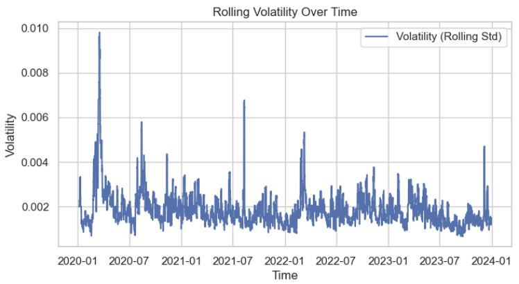
The volatility can be easily calculated with this line:

data['volatility'] = data['returns'].rolling(window=50).std()

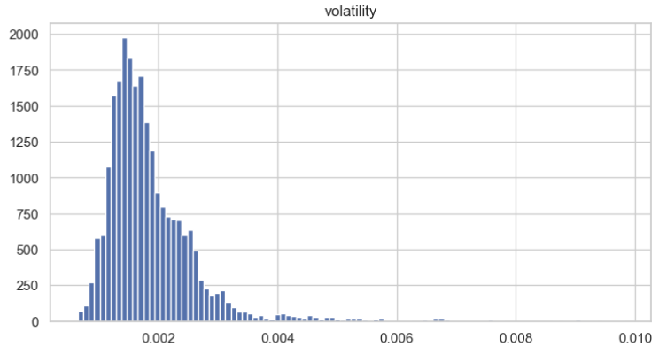
Next, we visualize the volatility distribution to better understand its features. We can see clearly that it approximately follows normal distribution.

We use the Augmented Dickey-Fuller (ADF) test to validate that the volatility data is stationary. The test should most likely produce the following result:

Augmented Dickey-Fuller Test: Volatility
ADF Statistic: -13.120552520156329
p-value: 1.5664189630119278e-24
# Lags Used: 46
Number of Observations Used: 23516
=> The series is likely stationary.

Although Hidden Markov Models (HMMs) are not strictly necessary for stationary data due to their rolling update behavior, having stationary data significantly benefits the clustering process and improves model precision.

Despite the volatility data is likely stationary and normally distributed, we still want to normalize it to a standard normal distribution so that the range becomes more tractable. 

In statistics, this process is called "scaling," where any normally distributed random variable x can be transformed to a standard normal distribution N(0,1) using the following operation:

Here, μ represents the mean and σ represents the standard deviation of x.

Keep in mind that later, when integrating back into the MetaTrader 5 editor, we will need to perform the same normalization operations. That's why we also need to store the mean and standard deviation.

from sklearn.preprocessing import StandardScaler
scaler = StandardScaler()
scaled_volatility = scaler.fit_transform(data[['volatility']])
scaled_volatility = scaled_volatility.reshape(-1, 1)
scaler_mean = scaler.mean_[0]  # Mean of the volatility feature
scaler_std = scaler.scale_[0]  # Standard deviation of the volatility feature

Then, we train the model on the scaled volatility data like this:

from hmmlearn import hmm
import numpy as np
# Define the number of hidden states
n_states = 2
# Initialize the Gaussian HMM
model = hmm.GaussianHMM(n_components=n_states, covariance_type="full", n_iter=100, random_state=42, verbose = True)
# Fit the model to the scaled volatility data
model.fit(scaled_volatility)

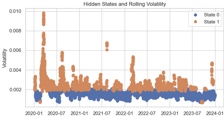
When predicting the hidden states for each training data point, the cluster distribution appears quite reasonable, with only minor errors.

# Predict the hidden states
hidden_states = model.predict(scaled_volatility)

# Add the hidden states to your dataframe
data['hidden_state'] = hidden_states
plt.figure(figsize=(14, 6))
for state in range(n_states):
    state_mask = data['hidden_state'] == state
    plt.plot(data.index[state_mask], data['volatility'][state_mask], 'o', label=f'State {state}')
plt.title('Hidden States and Rolling Volatility')
plt.xlabel('Time')
plt.ylabel('Volatility')
plt.legend()
plt.show()

Finally, we format the desired output into MQL5 language, and save them into a JSON header file, making it easier to copy and paste the corresponding matrix values into the MetaTrader 5 editor.

import json

# Your HMM model parameters
transition_matrix = model.transmat_
means = model.means_
covars = model.covars_

# Construct the data in the required format
data = {
    "A": [
        [transition_matrix[0, 0], transition_matrix[0, 1]],
        [transition_matrix[1, 0], transition_matrix[1, 1]]
    ],
    "mu": [means[0, 0], means[1, 0]],
    "sigma_sq": [covars[0, 0], covars[1, 0]],
    "scaler_mean": scaler_mean,
    "scaler_std": scaler_std
}

# Create the output content in the desired format
output_str = """
const double A[2][2] = { 
    {%.16f, %.16f}, 
    {%.16f, %.16f}
};
const double mu[2] = {%.16f, %.16f};
const double sigma_sq[2] = {%.16f, %.16f};
const double scaler_mean = %.16f;
const double scaler_std = %.16f;
""" % (
    data["A"][0][0], data["A"][0][1], data["A"][1][0], data["A"][1][1],
    data["mu"][0], data["mu"][1],
    data["sigma_sq"][0], data["sigma_sq"][1],
    data["scaler_mean"], data["scaler_std"]
)

# Write to a file
with open('model_parameters.h', 'w') as f:
    f.write(output_str)

print("Parameters saved to model_parameters.h")

The resulted file should look something like this:

const double A[2][2] = { 
    {0.9941485184089348, 0.0058514815910651}, 
    {0.0123877225858242, 0.9876122774141759}
};
const double mu[2] = {-0.4677410059727503, 0.9797900996225393};
const double sigma_sq[2] = {0.1073520489683212, 1.4515804806463273};
const double scaler_mean = 0.0018685496675093;
const double scaler_std = 0.0008350190448735;

We should paste them into our EA's code as global variables.

Integration

Now, let's head back to the MetaTrader 5 code editor and build on top of our original strategy code.

We first need to create functions to calculate the rolling volatility that keeps updating.

//+------------------------------------------------------------------+
//| Get volatility Function                                          |
//+------------------------------------------------------------------+
void GetVolatility(){
// Step 1: Get the last two close prices to compute the latest percent change
        double close_prices[2];
        int copied = CopyClose(_Symbol, PERIOD_CURRENT, 1, 2, close_prices);
        if(copied != 2){
            Print("Failed to copy close prices. Copied: ", copied);
            return;
        }
        
        // Step 2: Compute the latest percent change
        double latest_close = close_prices[0];
        double previous_close = close_prices[1];
        double percent_change = 0.0;
        if(previous_close != 0){
            percent_change = (latest_close - previous_close) / previous_close;
        }
        else{
            Print("Previous close price is zero. Percent change set to 0.");
        }
        
        // Step 3: Update the percent_changes buffer
        percent_changes[percent_change_index] = percent_change;
        percent_change_index++;
        if(percent_change_index >= 50){
            percent_change_index = 0;
            percent_change_filled = true;
        }
        
        // Step 4: Once the buffer is filled, compute the rolling std dev
        if(percent_change_filled){
            double current_stddev = ComputeStdDev(percent_changes, 50);
            // Step 5: Scale the std dev
            double scaled_stddev = (current_stddev - scaler_mean) / scaler_std;
            
            // Step 6: Update the volatility array (ring buffer for Viterbi)
            // Shift the volatility array to make room for the new std dev
            for(int i = 0; i < 49; i++){
                volatility[i] = volatility[i+1];
            }
            volatility[49] = scaled_stddev; // Insert the latest std dev
       }
}

//+------------------------------------------------------------------+
//| Compute Standard Deviation Function                              |
//+------------------------------------------------------------------+
double ComputeStdDev(double &data[], int size)
{
    if(size <= 1)
        return 0.0;
    
    double sum = 0.0;
    double sum_sq = 0.0;
    for(int i = 0; i < size; i++)
    {
        sum += data[i];
        sum_sq += data[i] * data[i];
    }
    double mean = sum / size;
    double variance = (sum_sq - (sum * sum) / size) / (size - 1);
    return MathSqrt(variance);
}

• GetVolatility() computes and tracks rolling volatility over time by using the scaled standard deviation of percentage price changes.
• ComputeDtsDev() serves as a helper function to calculate the standard deviation of a given data array. 

Then, we write two functions that calculate the current hidden state based on our matrices and the current rolling volatility.

//+------------------------------------------------------------------+
//| Viterbi Algorithm Implementation in MQL5                         |
//+------------------------------------------------------------------+
int Viterbi(double &obs[], int &states[])
{
    // Initialize dynamic programming tables
    double T1[2][50];
    int T2[2][50];

    // Initialize first column
    for(int s = 0; s < 2; s++)
    {
         double emission_prob = (1.0 / MathSqrt(2 * M_PI * sigma_sq[s])) * MathExp(-MathPow(obs[0] - mu[s], 2) / (2 * sigma_sq[s])) + 1e-10;

        T1[s][0] = MathLog(pi[s]) + MathLog(emission_prob);
        T2[s][0] = 0;
    }

    // Fill the tables
    for(int t = 1; t < 50; t++)
    {
        for(int s = 0; s < 2; s++)
        {
            double max_prob = -DBL_MAX; // Initialize to negative infinity
            int max_state = 0;
            for(int s_prev = 0; s_prev < 2; s_prev++)
            {
                double transition_prob = A[s_prev][s];
                if(transition_prob <= 0) transition_prob = 1e-10; // Prevent log(0)
                double prob = T1[s_prev][t-1] + MathLog(transition_prob);
                if(prob > max_prob)
                {
                    max_prob = prob;
                    max_state = s_prev;
                }
            }
            // Calculate emission probability with epsilon
            double emission_prob = (1.0 / MathSqrt(2 * M_PI * sigma_sq[s])) * MathExp(-MathPow(obs[t] - mu[s], 2) / (2 * sigma_sq[s])) + 1e-10;
            T1[s][t] = max_prob + MathLog(emission_prob);
            T2[s][t] = max_state;
        }
    }

    // Backtrack to find the optimal state sequence
    // Find the state with the highest probability in the last column
    double max_final_prob = -DBL_MAX;
    int last_state = 0;
    for(int s = 0; s < 2; s++)
    {
        if(T1[s][49] > max_final_prob)
        {
            max_final_prob = T1[s][49];
            last_state = s;
        }
    }    
    // Initialize the states array
    ArrayResize(states, 50);
    states[49] = last_state;
    // Backtrack
    for(int t = 48; t >= 0; t--)
    {
        states[t] = T2[states[t+1]][t+1];
    }
    return 0; // Success
}

//+------------------------------------------------------------------+
//| Predict Current Hidden State                                     |
//+------------------------------------------------------------------+
int PredictCurrentState(double &obs[])
{   
    // Define states array
    int states[50];
    
    // Apply Viterbi
    int ret = Viterbi(obs, states);
    if(ret != 0)
        return -1; // Error
    
    // Return the most probable current state
    return states[49];
}

The Viterbi() function implements the Viterbi algorithm, a dynamic programming method for finding the most probable sequence of hidden states in a Hidden Markov Model (HMM) given the observed data (obs[]).

1. Initialization:

• Dynamic Programming Tables:

  • T1[s][t] : Log-probability of the most probable state sequence that ends in state s at time t.
  • T2[s][t] : Pointer table storing the state that maximized the probability of transitioning to state s at time t.

• First Time Step (t = 0):

  • Compute the initial probabilities using the prior probabilities of each state (π[s]) and the emission probabilities for the first observation (obs[0]).

2. Recursive Calculation:

For each time step t from 1 to 49 :

1. For each state s:

   Compute the maximum probability of transitioning from any previous state s_prev to s using the following equation:               

   

   Here, the transition probability A[s_prev, s] is converted to log-space to avoid numerical underflow.

2. Store the state s_prev that maximized the probability in T2[s][t].

3. Backtracking to Retrieve the Optimal Path:

1. Start from the state with the highest probability at the last time step (t = 49).
2. Trace back through T2 to reconstruct the most probable sequence of states, storing the result in states[].

The final output is states[] which contains the most probable state sequence.

The PredictCurrentState() function utilizes the Viterbi() function to predict the current hidden state based on observations.

1. For initialization, it defines an array states[50] to store the result from Viterbi().
2. Then it passes the observation sequence obs[] to the Viterbi() function to compute the most probable sequence of hidden states.
3. Lastly, it returns the state at the last time step (states[49]), which represents the most probable current hidden state.

If you're confused by the mathematics behind this, I highly recommend checking out some more intuitive illustrations on the internet. Here, I'll try to briefly explain what we're doing.

The observed states are the scaled volatility data, which we can obtain and store in the obs[] array, containing 50 elements in this case. These elements correspond to y1, y2, ... y50 in the diagram. The corresponding hidden states can be either 0 or 1, representing the abstract conditions of current volatility (high or low).

These hidden states are determined through clustering during the model training process we performed earlier in Python. It's important to note that the Python code doesn't know exactly what each number represents—it only knows how to cluster the data and identify the features of the transition properties between states.

Initially, we randomly assign a state to x1, assuming each state has an equal weight. If we don't want to make this assumption, we could calculate the stationary distribution of the initial state using our training data, which would be the eigenvector of the transition matrix. For simplicity, we assume the stationary distribution vector to be [0.5, 0.5].

Through the training of the Hidden Markov Model, we obtain the probability of transitioning to a different hidden state and the probability of emitting a different observation. Using Bayes' Theorem, we can calculate the probability of all possible paths for each Markov chain and determine the most probable path. This allows us to find the most likely outcome for x50, the final hidden state in the sequence.

Finally, we adjust the original OnTick() logic by calculating the hidden states for each close and adding an entry criterion that the hidden state must equal 1.

//+------------------------------------------------------------------+
//| Check Volatility is filled Function                              |
//+------------------------------------------------------------------+
bool IsVolatilityFilled(){
     bool volatility_filled = true;
     for(int i = 0; i < 50; i++){
         if(volatility[i] == 0){
             volatility_filled = false;
             break;
         }
     }
     if(!volatility_filled){
         Print("Volatility buffer not yet filled.");
         return false;
     }
     else return true;
}  

//+------------------------------------------------------------------+
//| Expert tick function                                             |
//+------------------------------------------------------------------+
void OnTick()
  {
  int bars = iBars(_Symbol,PERIOD_CURRENT);
  if (barsTotal!= bars){
     barsTotal = bars;
     double maFast[];
     double maSlow[];
     double ma[];  
     
     GetVolatility();
     if(!IsVolatilityFilled()) return;
     int currentState = PredictCurrentState(volatility);
     
     CopyBuffer(handleMaFast,BASE_LINE,1,2,maFast);
     CopyBuffer(handleMaSlow,BASE_LINE,1,2,maSlow);
     CopyBuffer(handleMa,0,1,1,ma);

     double bid = SymbolInfoDouble(_Symbol, SYMBOL_BID);
     double ask = SymbolInfoDouble(_Symbol, SYMBOL_ASK);
     double lastClose = iClose(_Symbol, PERIOD_CURRENT, 1);
     //The order below matters
     if(buypos>0&& lastClose<maSlow[1]) trade.PositionClose(buypos);
     if(sellpos>0 &&lastClose>maSlow[1])trade.PositionClose(sellpos);        
     if (maFast[1]>maSlow[1]&&maFast[0]<maSlow[0]&&buypos ==sellpos&&currentState==1)executeBuy(); 
     if(maFast[1]<maSlow[1]&&maFast[0]>maSlow[0]&&sellpos ==buypos&&currentState==1) executeSell();
     
     if(buypos>0&&(!PositionSelectByTicket(buypos)|| PositionGetInteger(POSITION_MAGIC) != Magic)){
      buypos = 0;
      }
     if(sellpos>0&&(!PositionSelectByTicket(sellpos)|| PositionGetInteger(POSITION_MAGIC) != Magic)){
      sellpos = 0;
      }
    }
 }

Backtest

We trained the model using in-sample data from January 1, 2020, to January 1, 2024. Now, we want to test the results for the period from January 1, 2024, to January 1, 2025, on XAUUSD in the 1-hour timeframe.

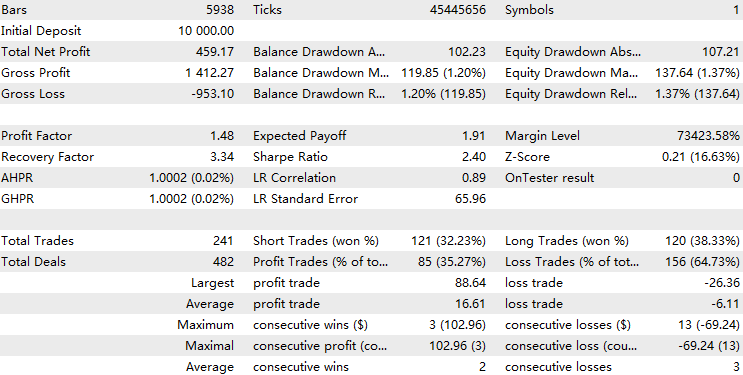
Firstly, we will compare the performance with the baseline, which is the result without integrating the HMM.

Now we perform a backtest of the EA with the HMM model filter implemented.

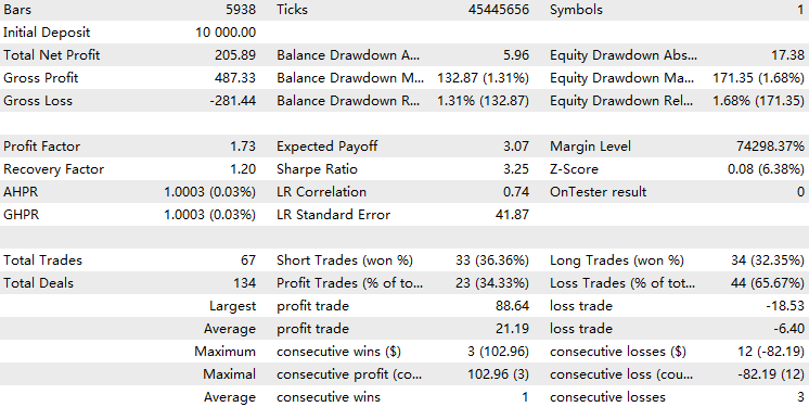
We can see that the EA with the HMM implementation filtered out about 70% of the total trades. It outperforms the baseline, with a profit factor of 1.73 compared to the baseline's 1.48, as well as a higher Sharpe ratio. This suggests that the HMM model we trained exhibits some level of predictability.

If we perform a rolling backtest, where we repeat this 4-year training and 1-year testing procedure starting from 2004, and compile all the results into one equity curve, we will get a result like this:

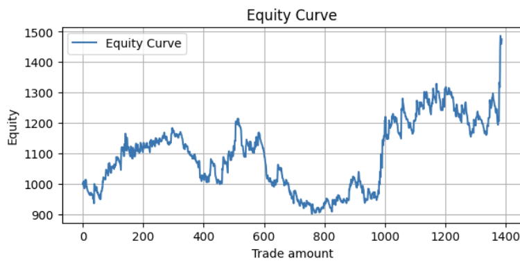
Metrics:

Profit Factor: 1.10
Maximum Drawdown: -313.17
Average Win: 11.41
Average Loss: -5.01
Win Rate: 32.56%

This is quite profitable with some space for improvement.

Reflections

In the current trading world, which is dominated by machine learning methods, there is an ongoing debate about whether to use more complex models, such as Recurrent Neural Networks (RNNs), or to stick with simpler models, like Hidden Markov Models (HMMs).

Pros:

1. Simplicity: Easier to implement and interpret compared to complex models like RNN which introduces ambiguity of what each parameter and operation represents.
2. Less Data Requirement: Requires fewer training samples to estimate model parameters, and require less computing power.
3. Fewer parameters: More resilient towards overfitting issues.

Cons:

1. Limited Complexity: May fail to capture intricate patterns in volatile data that RNNs can model.
2. Assumption of Markov Process: Assumes volatility transitions are memoryless, which may not hold in real markets.
3. Overfitting Risk: Despite its simplicity, if too many states are involved, HMM would still be prone to overfitting.

It is a popular approach to predict volatility rather than prices using machine learning methods, as scholars have found volatility predictions to be more reliable. However, a limitation in the approach introduced in this article is that the observations we fetch every new bar (50-period rolling average volatility) and the hidden states we define (high/low volatility states) are somewhat correlated, leading to reduced prediction significance. This suggests that similar results might have been achieved by simply using the observation data as filters.

For future development, I encourage readers to explore other definitions for hidden states, as well as experiment with more than two states to improve the model's robustness and prediction power.

Conclusion

In this article, we first explained the motivation for utilizing HMMs as a volatility state predictor for a trend-following strategy, while also introducing the basic concept of HMM. Next, we walked through the entire strategy development process, which included developing a backbone strategy in MQL5 using MetaTrader 5, fetching data, and training the HMMs in Python, followed by integrating the models back into MetaTrader 5. Afterward, we performed a backtest and analyzed its performance, briefly explaining the mathematical logic behind HMMs through a diagram. Finally, I shared my reflections on the strategy, along with aspirations for future development on top of this framework.

File Table

File Name	Usage
HMM Test.mq5	The trading EA implementation
Classic Trend Following.mq5	The baseline strategy EA
OHLC Getter.mq5	The EA for fetching data
FileCSV.mqh	The Include file for storing data in CSV
rollingBacktest.ipynb	For training model and obtaining matrices