
Data Science and Machine Learning (Part 20): Algorithmic Trading Insights, A Faceoff Between LDA and PCA in MQL5

-- The more you have, The less you see!
What is Linear Discriminant Analysis(LDA)?
LDA is a supervised generalization machine learning algorithm that aims to find a linear combination of features that best separates the classes in a dataset.
Just like the Principal Component Analysis (PCA), it is a dimension reduction algorithm. These algorithms are a common choice for dimensionality reduction, in this article we are going to compare them and observe in what situation each algorithm works best. We already discussed the PCA in the prior articles of this series. Let us commence by observing what the LDA algorithm is all about as we will discuss it mostly, finally we will compare their performances on a simple dataset and in the strategy tester, make sure you stick to the end for awesome data science stuff.

Objectives/Theory:
The objectives of Linear Discriminant Analysis (LDA) include:
- Maximizing Class Separability: LDA aims to find linear combinations of features that maximize the separation between classes in the data. By projecting the data onto these discriminative dimensions, LDA helps to increase the distinction between different classes, making classification more effective.
- Reducing Dimensionality: LDA reduces the dimensionality of the feature space by projecting the data onto a lower-dimensional subspace. This dimensionality reduction is achieved while preserving as much class-discriminatory information as possible. The reduced feature space can lead to simpler models, faster computation, and improved generalization performance.
- Minimizing Within-Class Variability: LDA aims to minimize the within-class scatter or variability by ensuring that data points belonging to the same class are tightly clustered together in the transformed space. By reducing within-class variability, LDA helps to enhance the separability between classes and improve the robustness of the classification model.
- Maximizing Between-Class Variability: Conversely, LDA seeks to maximize the between-class scatter or variability by maximizing the distance between the class means in the transformed space. By maximizing between-class variability while minimizing within-class variability, LDA achieves better discrimination between classes, leading to more accurate classification results.
- Handling Multiclass Classification: LDA can handle multiclass classification problems where there are more than two classes. By considering the relationships between all classes simultaneously, LDA finds a common subspace that optimally separates all classes, leading to effective classification boundaries in high-dimensional feature spaces.
Assumptions:
Linear Discriminant Analysis makes several assumptions, take a look a thousands of protein dataset, It assumes that.
- Measurements are independent from each other
- Data is normally distributed within the features
- The classes in the dataset have the same co-variance matrix
Steps in the Linear Discriminant Algorithm
01: Compute the Within-Class Scatter Matrix (SW)
Calculate the scatter matrices for each class.
  matrix SW, SB; //within and between scatter matrices
  SW.Init(num_features, num_features);
  SB.Init(num_features, num_features);

  for (ulong i=0; i<num_classes; i++)
   {
     matrix class_samples = {};
      for (ulong j=0, count=0; j<x.Rows(); j++)
         {
           if (y[j] == classes[i]) //Collect a matrix for samples belonging to a particular class
            {
               count++;
               class_samples.Resize(count, num_features);
               class_samples.Row(x.Row(j), count-1);
            }
         }


     matrix diff = Base::subtract(class_samples, class_means.Row(i)); //Each row subtracted to the mean
     if (diff.Rows()==0 && diff.Cols()==0) //if the subtracted matrix is zero stop the program for possible bugs or errors
      {
        DebugBreak();
        return x_centered;
      }

     SW += diff.Transpose().MatMul(diff); //Find within scatter matrix

     vector mean_diff = class_means.Row(i) - x_centered.Mean(0);
     SB += class_samples.Rows() * mean_diff.Outer(mean_diff); //compute between scatter matrix
   }
Sum these individual scatter matrices to get the within-class scatter matrix.
02: Compute the Between-Class Scatter Matrix (SB)
Calculate the mean vector for each class.
  matrix SW, SB; //within and between scatter matrices
  SW.Init(num_features, num_features);
  SB.Init(num_features, num_features);

  for (ulong i=0; i<num_classes; i++)
   {

     matrix class_samples = {};
      for (ulong j=0, count=0; j<x.Rows(); j++)
         {
           if (y[j] == classes[i]) //Collect a matrix for samples belonging to a particular class
            {
               count++;
               class_samples.Resize(count, num_features);
               class_samples.Row(x.Row(j), count-1);
            }
         }

     matrix diff = Base::subtract(class_samples, class_means.Row(i)); //Each row subtracted to the mean
     if (diff.Rows()==0 && diff.Cols()==0) //if the subtracted matrix is zero stop the program for possible bugs or errors
      {
        DebugBreak();
        return x_centered;
      }

     SW += diff.Transpose().MatMul(diff); //Find within scatter matrix

     vector mean_diff = class_means.Row(i) - x_centered.Mean(0);
     SB += class_samples.Rows() * mean_diff.Outer(mean_diff); //compute between scatter matrix
   }
Calculate the between-class scatter matrix.
SB += class_samples.Rows() * mean_diff.Outer(mean_diff); //compute between scatter matrix 03: Compute Eigenvalues and Eigenvectors:
Solve the generalized eigenvalue problem involving SW and SB obtain the eigenvalues and their corresponding eigenvectors.
  matrix eigen_vectors;
  vector eigen_values;

  matrix SBSW = SW.Inv().MatMul(SB);

  SBSW += this.m_regparam * MatrixExtend::eye((uint)SBSW.Rows());

  if (!SBSW.Eig(eigen_vectors, eigen_values))
    {
      Print("%s Failed to calculate eigen values and vectors Err=%d",__FUNCTION__,GetLastError());
      DebugBreak();

      matrix empty = {};
      return empty;
    }
Select Discriminative Features
Sort the eigenvalues in descending order.
   vector args = MatrixExtend::ArgSort(eigen_values);
   MatrixExtend::Reverse(args);

   eigen_values = Base::Sort(eigen_values, args);
   eigen_vectors = Base::Sort(eigen_vectors, args);
Choose the top k eigenvectors to form the transformation matrix.
this.m_components = extract_components(eigen_values); Since both Linear Discriminant analysis and the Principal Component Analysis serve similar purpose of dimensionality reduction we can use similar techniques to extract components such as variance and the Scree Plot just like the ones we used in the PCA article.
We can extend our LDA class to be capable of extracting components for itself when the NULL number of components is selected by default.
  if (this.m_components == NULL)
    this.m_components = extract_components(eigen_values);
  else //plot the scree plot
    extract_components(eigen_values);
Project Data onto New Feature Space
Multiply the original data by the selected eigenvectors to obtain the new feature space.
  this.projection_matrix = Base::Slice(eigen_vectors, this.m_components);

  return x_centered.MatMul(projection_matrix.Transpose());
All this code is executed inside the function fit_transform which is the function responsible for training and preparing the Linear Discriminant Analysis algorithm. To make our class capable of handling new/unseen data we need to add the functions for further transformations.
matrix CLDA::transform(const matrix &x)
 {
   if (this.projection_matrix.Rows() == 0)
    {
      printf("%s fit_transform method must be called befor transform",__FUNCTION__);
      matrix empty = {};
      return empty;
    }
  matrix x_centered = Base::subtract(x, this.mean);

  return x_centered.MatMul(this.projection_matrix.Transpose());
 }
//+------------------------------------------------------------------+
//|                                                                  |
//+------------------------------------------------------------------+
vector CLDA::transform(const vector &x)
 {
   matrix m = MatrixExtend::VectorToMatrix(x, this.num_features);

   if (m.Rows()==0)
    {
      vector empty={};
      return empty; //return nothing since there is a failure in converting vector to matrix
    }

   m = transform(m);
   return MatrixExtend::MatrixToVector(m);
 }
LDA class overview
Our overall LDA class now looks like below:
enum lda_criterion //selecting best components criteria selection
  {
    CRITERION_VARIANCE,
    CRITERION_KAISER,
    CRITERION_SCREE_PLOT
  };

class CLDA
  {
CPlots   plt;

protected:
   uint m_components;
   lda_criterion m_criterion;

   matrix projection_matrix;
   ulong num_features;
   double m_regparam;
   vector mean;

   uint CLDA::extract_components(vector &eigen_values, double threshold=0.95);

public:
                     CLDA(uint k=NULL, lda_criterion CRITERION_=CRITERION_SCREE_PLOT, double reg_param =1e-6);
                    ~CLDA(void);

                     matrix fit_transform(const matrix &x, const vector &y);
                     matrix transform(const matrix &x);
                     vector transform(const vector &x);
  };
The reg_param which stands for regularization parameter is of less importance knowing, that it only helps regularize SW and SB matrices to make the eigenvalues and vectors calculations less error-prone.
   SW += this.m_regparam * MatrixExtend::eye((uint)num_features);
   SB += this.m_regparam * MatrixExtend::eye((uint)num_features);
Using Linear Discriminant Analysis On a Dataset
Let us apply our LDA class to the popular Iris dataset and observe what it does.
   string headers;
   matrix data = MatrixExtend::ReadCsv("iris.csv",headers); //Read csv
Remember this is a supervised machine learning technique, meaning that we have to collect the independent and target variables separately and give them to a model.
   matrix x;
   vector y;
   MatrixExtend::XandYSplitMatrices(data, x, y);
#include <MALE5\Dimensionality Reduction\LDA.mqh>

CLDA *lda;
//+------------------------------------------------------------------+
//| Expert initialization function                                   |
//+------------------------------------------------------------------+
int OnInit()
  {
//---

   string headers;
   matrix data = MatrixExtend::ReadCsv("iris.csv",headers); //Read csv

   matrix x;
   vector y;
   MatrixExtend::XandYSplitMatrices(data, x, y);

   Print("Original X\n",x);

   lda = new CLDA();
   matrix transformed_x = lda.fit_transform(x, y);

   Print("Transformed X\n",transformed_x);

   return(INIT_SUCCEEDED);
  }
Outputs
HH      0       10:18:21.210    LDA Test (EURUSD,H1)    Original X
IQ      0       10:18:21.210    LDA Test (EURUSD,H1)    [[5.1,3.5,1.4,0.2]
HF      0       10:18:21.210    LDA Test (EURUSD,H1)     [4.9,3,1.4,0.2]
...
...
ES      0       10:18:21.211    LDA Test (EURUSD,H1)     [6.5,3,5.2,2]
ML      0       10:18:21.211    LDA Test (EURUSD,H1)     [6.2,3.4,5.4,2.3]
EI      0       10:18:21.211    LDA Test (EURUSD,H1)     [5.9,3,5.1,1.8]]
IL      0       10:18:21.243    LDA Test (EURUSD,H1)
DD      0       10:18:21.243    LDA Test (EURUSD,H1)    Transformed X
DM      0       10:18:21.243    LDA Test (EURUSD,H1)    [[-1.058063221542643,2.676898315513957]
JD      0       10:18:21.243    LDA Test (EURUSD,H1)     [-1.060778666796316,2.532150351483708]
DM      0       10:18:21.243    LDA Test (EURUSD,H1)     [-0.9139922886488467,2.777963946569435]
...
...
IK      0       10:18:21.244    LDA Test (EURUSD,H1)     [1.527279343196588,-2.300606221030168]
QN      0       10:18:21.244    LDA Test (EURUSD,H1)     [0.9614855249192527,-1.439559895222919]
EF      0       10:18:21.244    LDA Test (EURUSD,H1)     [0.6420061576026481,-2.511057690832021…]
A beautiful scree plot was shown on the chart too:
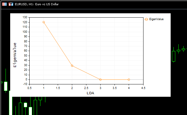
From the scree plot we can see the best number of components is at the elbow point which is 2, and that is exactly the number of components our class returned, awesome. Now let us visualize the components returned to see if they are distinctive, as we all know that the purpose of reducing dimensions is to get the minimum number of components that explains all the variance in the original data, simply put a simplified version of our data.
I decided to save the components from our EA into a csv file and plot them using python on this notebook https://www.kaggle.com/code/omegajoctan/lda-vs-pca-components-iris-data
MatrixExtend::WriteCsv("iris-data lda-components.csv",transformed_x); 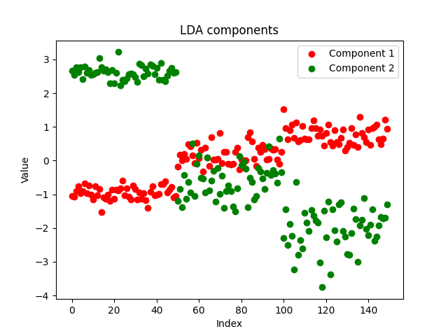
The components looks clean, indicating a successful implementation. Now let us see what the PCA components looks like:
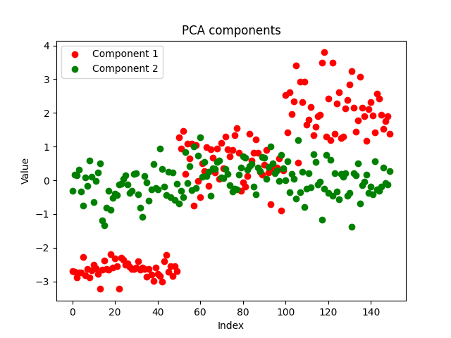
Both methods have separated the data well, We can't say which performed better by looking at the plot, let us use the same model under the same parameters for the same dataset and observe the accuracy of both models on both training and out-of-sample testing.
LDA vs PCA during Train-Test
Using the decision tree model with the same parameters for two separate data obtained from LDA and PCA algorithms respectively.
#include <MALE5\Dimensionality Reduction\LDA.mqh>
#include <MALE5\Dimensionality Reduction\PCA.mqh>
#include <MALE5\Decision Tree\tree.mqh>
#include <MALE5\Metrics.mqh>

CLDA *lda;
CPCA *pca;
CDecisionTreeClassifier *classifier_tree;

input int random_state_ = 42;
input double training_sample_size = 0.7;
//+------------------------------------------------------------------+
//| Expert initialization function                                   |
//+------------------------------------------------------------------+
int OnInit()
  {
//---

   string headers;
   matrix data = MatrixExtend::ReadCsv("iris.csv",headers); //Read csv

   Print("<<<<<<<< LDA Applied >>>>>>>>>");

   matrix x_train, x_test;
   vector y_train, y_test;

   MatrixExtend::TrainTestSplitMatrices(data,x_train,y_train,x_test,y_test,training_sample_size,random_state_);

   lda = new CLDA(NULL);

   matrix x_transformed = lda.fit_transform(x_train, y_train); //Transform the training data

   classifier_tree = new CDecisionTreeClassifier();
   classifier_tree.fit(x_transformed, y_train); //Train the model using the transformed data

   vector preds = classifier_tree.predict(x_transformed); //Make predictions using the transformed data

   Print("Train accuracy: ",Metrics::confusion_matrix(y_train, preds).accuracy);

   x_transformed = lda.transform(x_test);
   preds = classifier_tree.predict(x_transformed);

   Print("Test accuracy: ",Metrics::confusion_matrix(y_test, preds).accuracy);

   delete (classifier_tree);
   delete (lda);

//---

   Print("<<<<<<<< PCA Applied >>>>>>>>>");

   pca = new CPCA(NULL);

   x_transformed = pca.fit_transform(x_train);

   classifier_tree = new CDecisionTreeClassifier();
   classifier_tree.fit(x_transformed, y_train);

   preds = classifier_tree.predict(x_transformed); //Make predictions using the transformed data

   Print("Train accuracy: ",Metrics::confusion_matrix(y_train, preds).accuracy);

   x_transformed = pca.transform(x_test);
   preds = classifier_tree.predict(x_transformed);

   Print("Test accuracy: ",Metrics::confusion_matrix(y_test, preds).accuracy);

   delete (classifier_tree);
   delete(pca);

   return(INIT_SUCCEEDED);
  }
LDA results
GM      0       18:23:18.285    LDA Test (EURUSD,H1)    <<<<<<<< LDA Applied >>>>>>>>>
MR      0       18:23:18.302    LDA Test (EURUSD,H1)
JP      0       18:23:18.344    LDA Test (EURUSD,H1)    Confusion Matrix
FK      0       18:23:18.344    LDA Test (EURUSD,H1)    [[39,0,0]
CR      0       18:23:18.344    LDA Test (EURUSD,H1)     [0,30,5]
QF      0       18:23:18.344    LDA Test (EURUSD,H1)     [0,2,29]]
IS      0       18:23:18.344    LDA Test (EURUSD,H1)
OM      0       18:23:18.344    LDA Test (EURUSD,H1)    Classification Report
KF      0       18:23:18.344    LDA Test (EURUSD,H1)
QQ      0       18:23:18.344    LDA Test (EURUSD,H1)    _    Precision  Recall  Specificity  F1 score  Support
FF      0       18:23:18.344    LDA Test (EURUSD,H1)    1.0    1.00     1.00     1.00       1.00     39.0
GI      0       18:23:18.344    LDA Test (EURUSD,H1)    2.0    0.94     0.86     0.97       0.90     35.0
ML      0       18:23:18.344    LDA Test (EURUSD,H1)    3.0    0.85     0.94     0.93       0.89     31.0
OS      0       18:23:18.344    LDA Test (EURUSD,H1)
FN      0       18:23:18.344    LDA Test (EURUSD,H1)    Accuracy                                   0.93
JO      0       18:23:18.344    LDA Test (EURUSD,H1)    Average   0.93    0.93    0.97      0.93    105.0
KJ      0       18:23:18.344    LDA Test (EURUSD,H1)    W Avg     0.94    0.93    0.97      0.93    105.0
EQ      0       18:23:18.344    LDA Test (EURUSD,H1)    Train accuracy: 0.933
JH      0       18:23:18.344    LDA Test (EURUSD,H1)    Confusion Matrix
LS      0       18:23:18.344    LDA Test (EURUSD,H1)    [[11,0,0]
IJ      0       18:23:18.344    LDA Test (EURUSD,H1)     [0,13,2]
RN      0       18:23:18.344    LDA Test (EURUSD,H1)     [0,1,18]]
IK      0       18:23:18.344    LDA Test (EURUSD,H1)
OE      0       18:23:18.344    LDA Test (EURUSD,H1)    Classification Report
KN      0       18:23:18.344    LDA Test (EURUSD,H1)
QI      0       18:23:18.344    LDA Test (EURUSD,H1)    _    Precision  Recall  Specificity  F1 score  Support
LN      0       18:23:18.344    LDA Test (EURUSD,H1)    1.0    1.00     1.00     1.00       1.00     11.0
CQ      0       18:23:18.344    LDA Test (EURUSD,H1)    2.0    0.93     0.87     0.97       0.90     15.0
QD      0       18:23:18.344    LDA Test (EURUSD,H1)    3.0    0.90     0.95     0.92       0.92     19.0
OK      0       18:23:18.344    LDA Test (EURUSD,H1)
FF      0       18:23:18.344    LDA Test (EURUSD,H1)    Accuracy                                   0.93
GD      0       18:23:18.344    LDA Test (EURUSD,H1)    Average   0.94    0.94    0.96      0.94    45.0
HQ      0       18:23:18.344    LDA Test (EURUSD,H1)    W Avg     0.93    0.93    0.96      0.93    45.0
CF      0       18:23:18.344    LDA Test (EURUSD,H1)    Test accuracy: 0.933
LDA produced a stable model with 93% accuracy on both training and testing, let us look at the PCA.
PCA results:
MM      0       18:26:40.994    LDA Test (EURUSD,H1)    <<<<<<<< PCA Applied >>>>>>>>>

LS      0       18:26:41.071    LDA Test (EURUSD,H1)    Confusion Matrix
LJ      0       18:26:41.071    LDA Test (EURUSD,H1)    [[39,0,0]
ER      0       18:26:41.071    LDA Test (EURUSD,H1)     [0,34,1]
OE      0       18:26:41.071    LDA Test (EURUSD,H1)     [0,4,27]]
KD      0       18:26:41.071    LDA Test (EURUSD,H1)
IL      0       18:26:41.071    LDA Test (EURUSD,H1)    Classification Report
MG      0       18:26:41.071    LDA Test (EURUSD,H1)
CR      0       18:26:41.071    LDA Test (EURUSD,H1)    _    Precision  Recall  Specificity  F1 score  Support
DE      0       18:26:41.071    LDA Test (EURUSD,H1)    1.0    1.00     1.00     1.00       1.00     39.0
EH      0       18:26:41.071    LDA Test (EURUSD,H1)    2.0    0.89     0.97     0.94       0.93     35.0
KL      0       18:26:41.071    LDA Test (EURUSD,H1)    3.0    0.96     0.87     0.99       0.92     31.0
ID      0       18:26:41.071    LDA Test (EURUSD,H1)
NO      0       18:26:41.071    LDA Test (EURUSD,H1)    Accuracy                                   0.95
CH      0       18:26:41.071    LDA Test (EURUSD,H1)    Average   0.95    0.95    0.98      0.95    105.0
KK      0       18:26:41.071    LDA Test (EURUSD,H1)    W Avg     0.95    0.95    0.98      0.95    105.0
NR      0       18:26:41.071    LDA Test (EURUSD,H1)    Train accuracy: 0.952
LK      0       18:26:41.071    LDA Test (EURUSD,H1)    Confusion Matrix
FR      0       18:26:41.071    LDA Test (EURUSD,H1)    [[11,0,0]
FJ      0       18:26:41.072    LDA Test (EURUSD,H1)     [0,14,1]
MM      0       18:26:41.072    LDA Test (EURUSD,H1)     [0,3,16]]
NL      0       18:26:41.072    LDA Test (EURUSD,H1)
HD      0       18:26:41.072    LDA Test (EURUSD,H1)    Classification Report
LO      0       18:26:41.072    LDA Test (EURUSD,H1)
FJ      0       18:26:41.072    LDA Test (EURUSD,H1)    _    Precision  Recall  Specificity  F1 score  Support
KM      0       18:26:41.072    LDA Test (EURUSD,H1)    1.0    1.00     1.00     1.00       1.00     11.0
EP      0       18:26:41.072    LDA Test (EURUSD,H1)    2.0    0.82     0.93     0.90       0.88     15.0
HD      0       18:26:41.072    LDA Test (EURUSD,H1)    3.0    0.94     0.84     0.96       0.89     19.0
HL      0       18:26:41.072    LDA Test (EURUSD,H1)
OG      0       18:26:41.072    LDA Test (EURUSD,H1)    Accuracy                                   0.91
PS      0       18:26:41.072    LDA Test (EURUSD,H1)    Average   0.92    0.93    0.95      0.92    45.0
IP      0       18:26:41.072    LDA Test (EURUSD,H1)    W Avg     0.92    0.91    0.95      0.91    45.0
PE      0       18:26:41.072    LDA Test (EURUSD,H1)    Test accuracy: 0.911
PCA gave a more accurate model providing 95% accuracy on training and 91.1% accuracy on testing.
Advantages of Linear Discriminant Analysis(LDA)
Linear Discriminant Analysis (LDA) offers several advantages, making it a widely used technique in classification and dimensionality reduction tasks:
- Helps in dimensionality reduction. LDA reduces the dimensionality of the feature space by transforming the original features into a lower-dimensional space. This reduction can lead to simpler models, alleviate the curse of dimensionality, and improve computational efficiency.
- Preserves class discriminatory information. LDA aims to find linear combinations of features that maximize the separation between classes. By focusing on the discriminative information that distinguishes between classes, LDA ensures that the transformed features retain important class-related patterns and structures.
- It extracts features and classifies them in one step. LDA simultaneously performs feature extraction and classification. It learns a transformation of the original features that maximizes class separability, making it inherently suited for classification tasks. This integrated approach can lead to more efficient and interpretable models.
- It is robust to overfitting. LDA is less prone to overfitting compared to other classification algorithms, especially when the number of samples is small relative to the number of features. By reducing the dimensionality of the feature space and focusing on the most discriminative features, LDA can generalize well to unseen data.
- Handles multi-class classification. LDA naturally extends to multiclass classification problems with more than two classes. It considers the relationships between all classes simultaneously, leading to effective separation boundaries in high-dimensional feature spaces.
- Computationally efficient. LDA involves solving eigenvalue problems and matrix multiplications, which are computationally efficient and can be implemented using built-in MQL5 methods. This makes LDA suitable for large-scale datasets and real-time applications.
- Easy to interprete. The transformed features obtained from LDA are interpretable and can be analyzed to understand the underlying patterns in the data. The linear combinations of features learned by LDA can provide insights into the discriminative factors driving the classification decision.
- Its assumptions are often met. LDA assumes that the data are normally distributed within each class with equal covariance matrices. While these assumptions may not always hold in practice, LDA can still perform well even when the assumptions are approximately met.
While Linear Discriminant Analysis (LDA) has several advantages, it also comes with some limitations and disadvantages:
Disadvantages of Linear Discriminant Analysis(LDA)
- It assumes Gaussian distribution within features. LDA assumes that the data within each class are normally distributed with equal covariance matrices. If this assumption is violated, LDA may produce suboptimal results or even fail to converge. In practice, real-world data may exhibit non-normal distributions, which can limit the effectiveness of LDA.
- Can be sensitive to outliers. LDA is sensitive to outliers, especially when the covariance matrices are estimated from limited data. Outliers can significantly affect the estimation of covariance matrices and the resulting discriminant directions, potentially leading to biased or unreliable classification results.
- Less flexible when modelling non-linear relationships. As it assumes that the decision boundaries between classes are linear. If the underlying relationships between features and classes are nonlinear, LDA may not capture these complex patterns effectively. In such cases, nonlinear dimensionality reduction techniques or nonlinear classifiers may be more appropriate.
- Curse of dimensionality is real. When the number of features is much larger than the number of samples, LDA may suffer from the curse of dimensionality. In high-dimensional feature spaces, the estimation of covariance matrices becomes less reliable, and the discriminant directions may not effectively capture the true underlying structure of the data.
- Limited Performance with Imbalanced Classes. LDA may perform poorly when dealing with imbalanced class distributions, where one or more classes have significantly fewer samples than others. In such cases, the class with fewer samples may be poorly represented in the estimation of class means and covariance matrices, leading to biased classification results.
- Can barely handle non-numeric data. LDA typically operates on numeric data, and it may not be directly applicable to datasets containing categorical or non-numeric variables. Preprocessing steps such as encoding categorical variables or transforming non-numeric data into numeric representations may be required, which can introduce additional complexity and potential information loss.
LDA vs PCA in the trading environment
To use these dimension reduction techniques in the trading environment, we have to make a function for training and testing the model of paper then we can use the trained model to make predictions on the strategy tester that will help us analyze their performance.
We will be using the 5 indicators in our dataset we would like to shrink using both of these methods:
int OnInit()
  {

//--- Trend following indicators

    indicator_handle[0] = iAMA(Symbol(), PERIOD_CURRENT, 9 , 2 , 30, 0, PRICE_OPEN);
    indicator_handle[1] = iADX(Symbol(), PERIOD_CURRENT, 14);
    indicator_handle[2] = iADXWilder(Symbol(), PERIOD_CURRENT, 14);
    indicator_handle[3] = iBands(Symbol(), PERIOD_CURRENT, 20, 0, 2.0, PRICE_OPEN);
    indicator_handle[4] = iDEMA(Symbol(), PERIOD_CURRENT, 14, 0, PRICE_OPEN);
 }
void TrainTest()
 {
   vector buffer = {};
   for (int i=0; i<ArraySize(indicator_handle); i++)
    {
      buffer.CopyIndicatorBuffer(indicator_handle[i], 0, 0, bars); //copy indicator buffer
      dataset.Col(buffer, i); //add the indicator buffer values to the dataset matrix
    }

//---

   vector y(bars);
   MqlRates rates[];
   CopyRates(Symbol(), PERIOD_CURRENT,0,bars, rates);
   for (int i=0; i<bars; i++) //Creating the target variable
     {
       if (rates[i].close > rates[i].open) //if bullish candle assign 1 to the y variable else assign the 0 class
        y[i] = 1;
       else
        y[0] = 0;
     }

//---

   dataset.Col(y, dataset.Cols()-1); //add the y variable to the last column

//---

   matrix x_train, x_test;
   vector y_train, y_test;

   MatrixExtend::TrainTestSplitMatrices(dataset,x_train,y_train,x_test,y_test,training_sample_size,random_state_);

   matrix x_transformed = {};
   switch(dimension_reduction)
     {
      case  LDA:

         lda = new CLDA(NULL);

         x_transformed = lda.fit_transform(x_train, y_train); //Transform the training data

        break;
      case PCA:

         pca = new CPCA(NULL);

         x_transformed = pca.fit_transform(x_train);

        break;
     }


   classifier_tree = new CDecisionTreeClassifier();
   classifier_tree.fit(x_transformed, y_train); //Train the model using the transformed data

   vector preds = classifier_tree.predict(x_transformed); //Make predictions using the transformed data

   Print("Train accuracy: ",Metrics::confusion_matrix(y_train, preds).accuracy);

   switch(dimension_reduction)
     {
      case  LDA:

        x_transformed = lda.transform(x_test); //Transform the testing data

        break;

      case PCA:

        x_transformed = pca.transform(x_test);

        break;
     }
   preds = classifier_tree.predict(x_transformed);

   Print("Test accuracy: ",Metrics::confusion_matrix(y_test, preds).accuracy);

 }
Once the data is trained it needs to be tested below was the outcome for both methods starting with LDA:
JK      0       01:00:24.440    LDA Test (EURUSD,H1)
GK      0       01:00:37.442    LDA Test (EURUSD,H1)    Confusion Matrix
QR      0       01:00:37.442    LDA Test (EURUSD,H1)    [[60,266]
FF      0       01:00:37.442    LDA Test (EURUSD,H1)     [46,328]]
DR      0       01:00:37.442    LDA Test (EURUSD,H1)
RN      0       01:00:37.442    LDA Test (EURUSD,H1)    Classification Report
FE      0       01:00:37.442    LDA Test (EURUSD,H1)
LP      0       01:00:37.442    LDA Test (EURUSD,H1)    _    Precision  Recall  Specificity  F1 score  Support
HD      0       01:00:37.442    LDA Test (EURUSD,H1)    0.0    0.57     0.18     0.88       0.28     326.0
FI      0       01:00:37.442    LDA Test (EURUSD,H1)    1.0    0.55     0.88     0.18       0.68     374.0
RM      0       01:00:37.442    LDA Test (EURUSD,H1)
QH      0       01:00:37.442    LDA Test (EURUSD,H1)    Accuracy                                   0.55
KQ      0       01:00:37.442    LDA Test (EURUSD,H1)    Average   0.56    0.53    0.53      0.48    700.0
HP      0       01:00:37.442    LDA Test (EURUSD,H1)    W Avg     0.56    0.55    0.51      0.49    700.0
KK      0       01:00:37.442    LDA Test (EURUSD,H1)    Train accuracy: 0.554
DR      0       01:00:37.443    LDA Test (EURUSD,H1)    Confusion Matrix
CD      0       01:00:37.443    LDA Test (EURUSD,H1)    [[20,126]
LO      0       01:00:37.443    LDA Test (EURUSD,H1)     [12,142]]
OK      0       01:00:37.443    LDA Test (EURUSD,H1)
ME      0       01:00:37.443    LDA Test (EURUSD,H1)    Classification Report
QN      0       01:00:37.443    LDA Test (EURUSD,H1)
GI      0       01:00:37.443    LDA Test (EURUSD,H1)    _    Precision  Recall  Specificity  F1 score  Support
JM      0       01:00:37.443    LDA Test (EURUSD,H1)    0.0    0.62     0.14     0.92       0.22     146.0
KR      0       01:00:37.443    LDA Test (EURUSD,H1)    1.0    0.53     0.92     0.14       0.67     154.0
MF      0       01:00:37.443    LDA Test (EURUSD,H1)
MQ      0       01:00:37.443    LDA Test (EURUSD,H1)    Accuracy                                   0.54
MJ      0       01:00:37.443    LDA Test (EURUSD,H1)    Average   0.58    0.53    0.53      0.45    300.0
OI      0       01:00:37.443    LDA Test (EURUSD,H1)    W Avg     0.58    0.54    0.52      0.45    300.0
QP      0       01:00:37.443    LDA Test (EURUSD,H1)    Test accuracy: 0.54
The PCA performed better during training but dropped a little bit during testing:
GE      0       01:01:57.202    LDA Test (EURUSD,H1)
MS      0       01:01:57.202    LDA Test (EURUSD,H1)    Classification Report
IH      0       01:01:57.202    LDA Test (EURUSD,H1)
OS      0       01:01:57.202    LDA Test (EURUSD,H1)    _    Precision  Recall  Specificity  F1 score  Support
KG      0       01:01:57.202    LDA Test (EURUSD,H1)    0.0    0.62     0.28     0.85       0.39     326.0
GL      0       01:01:57.202    LDA Test (EURUSD,H1)    1.0    0.58     0.85     0.28       0.69     374.0
MP      0       01:01:57.202    LDA Test (EURUSD,H1)
JK      0       01:01:57.202    LDA Test (EURUSD,H1)    Accuracy                                   0.59
HL      0       01:01:57.202    LDA Test (EURUSD,H1)    Average   0.60    0.57    0.57      0.54    700.0
CG      0       01:01:57.202    LDA Test (EURUSD,H1)    W Avg     0.60    0.59    0.55      0.55    700.0
EF      0       01:01:57.202    LDA Test (EURUSD,H1)    Train accuracy: 0.586
HO      0       01:01:57.202    LDA Test (EURUSD,H1)    Confusion Matrix
GG      0       01:01:57.202    LDA Test (EURUSD,H1)    [[26,120]
GJ      0       01:01:57.202    LDA Test (EURUSD,H1)     [29,125]]
KN      0       01:01:57.202    LDA Test (EURUSD,H1)
QJ      0       01:01:57.202    LDA Test (EURUSD,H1)    Classification Report
MQ      0       01:01:57.202    LDA Test (EURUSD,H1)
CL      0       01:01:57.202    LDA Test (EURUSD,H1)    _    Precision  Recall  Specificity  F1 score  Support
QP      0       01:01:57.202    LDA Test (EURUSD,H1)    0.0    0.47     0.18     0.81       0.26     146.0
GE      0       01:01:57.202    LDA Test (EURUSD,H1)    1.0    0.51     0.81     0.18       0.63     154.0
QI      0       01:01:57.202    LDA Test (EURUSD,H1)
MD      0       01:01:57.202    LDA Test (EURUSD,H1)    Accuracy                                   0.50
RE      0       01:01:57.202    LDA Test (EURUSD,H1)    Average   0.49    0.49    0.49      0.44    300.0
IL      0       01:01:57.202    LDA Test (EURUSD,H1)    W Avg     0.49    0.50    0.49      0.45    300.0
PP      0       01:01:57.202    LDA Test (EURUSD,H1)    Test accuracy: 0.503
Lastly we can create a simple trading strategy out of the signals provided by the decision tree model.
void OnTick()
  {
//---

   if (!train_once) //call the function to train the model once on the program lifetime
    {
      TrainTest();
      train_once = true;
    }

//---

   vector inputs(indicator_handle.Size());
   vector buffer;

   for (uint i=0; i<indicator_handle.Size(); i++)
     {
       buffer.CopyIndicatorBuffer(indicator_handle[i], 0, 0, 1); //copy the current indicator value
       inputs[i] = buffer[0]; //add its value to the inputs vector
     }

//---

    SymbolInfoTick(Symbol(), ticks);

     if (isnewBar(PERIOD_CURRENT)) // We want to trade on the bar opening
      {
        vector transformed_inputs = {};
         switch(dimension_reduction) //transform every new data to fit the dimensions selected during training
           {
            case  LDA:
               transformed_inputs = lda.transform(inputs); //Transform the new data
              break;
            case PCA:
               transformed_inputs = pca.transform(inputs);
              break;
           }

        int signal = (int)classifier_tree.predict(transformed_inputs);
        double min_lot = SymbolInfoDouble(Symbol(), SYMBOL_VOLUME_MIN);
        SymbolInfoTick(Symbol(), ticks);

         if (signal == -1)
           {
              if (!PosExists(MAGICNUMBER, POSITION_TYPE_SELL)) // If a sell trade doesnt exist
                m_trade.Sell(min_lot, Symbol(), ticks.bid, ticks.bid+stoploss*Point(), ticks.bid - takeprofit*Point());
           }
         else
           {
             if (!PosExists(MAGICNUMBER, POSITION_TYPE_BUY))  // If a buy trade doesnt exist
               m_trade.Buy(min_lot, Symbol(), ticks.ask, ticks.ask-stoploss*Point(), ticks.ask + takeprofit*Point());
           }
      }
  }
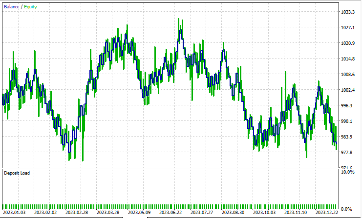
I ran a test in Open Prices Mode from 2023 January to 2024 February on Both methods applied to the simple strategy:
Linear Discriminant Analysis(LDA)

A test on Principal Component Analysis (PCA):
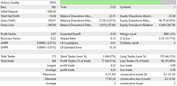
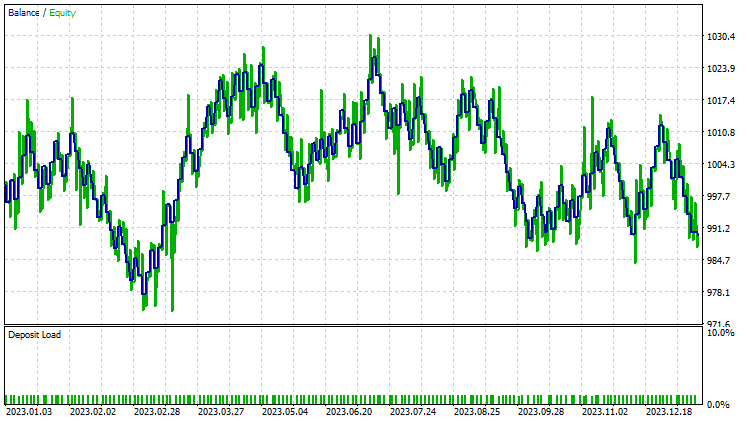
They performed almost the same with LDA making an 8$ loss more than the PCA, While the strategy tester is something every MQL5 trader looks at from a data scientist's angle of view, it is less relevant for these dimensional reduction techniques as their primary job is to simplify the variables especially when working with big data. I also have to explain that when running this EA on the strategy tester I experienced some inconsistencies in the calculations caused by bugs which are unexplored in matrices and vector methods, kindly run the program several times until you get meaningful outcome if you encounter errors and obstacles along the way.
if you have been reading this article series you might be asking yourself why we haven't scaled the transformed data obtained from these two techniques just like we did in the prior article.
Whether the data from PCA or LDA needs to be normalized for a machine learning model depends on the specific characteristics of your dataset, the algorithm you're using, and your objectives. Below are some things to consider:
- PCA Transformation; These two operates on the covariance matrix of the original features and finds orthogonal components (principal components) that capture the maximum variance in the data. The transformed data obtained from these two methods consists of these principal components.
- Normalization Prior to PCA or LDA; It's common practice to normalize the original features before performing PCA or LDA, especially if the features have different scales or units. Normalization ensures that all features contribute equally to the covariance matrix and prevents features with larger scales from dominating the principal components.
- Normalization After PCA or LDA; Whether you need to normalize the transformed data from PCA depends on the specific requirements of your machine learning algorithm and the characteristics of the transformed features. Some algorithms, such as logistic regression or k-nearest neighbors, are sensitive to differences in feature scales and may benefit from normalized features, even after PCA or LDA.
- Other algorithms, such as decision trees we have deployed or random forests, are less sensitive to feature scales and may not require normalization after PCA.
- Impact of Normalization on Interpretability; Normalization after PCA may affect the interpretability of the principal components. If you're interested in understanding the contributions of the original features to the principal components, normalizing the transformed data may obscure these relationships.
- Impact on Performance; Experiment with both normalized and unnormalized transformed data to assess the impact on model performance. In some cases, normalization may lead to better convergence, improved generalization, or faster training, while in other cases, it may have little to no effect.
Track development of machine learning models and much more discussed in this article series on this GitHub repo.
Attachments:
| File | Description/Usage |
|---|---|
| tree.mqh | Contains the decision tree classifier model |
| MatrixExtend.mqh | Has additional functions for matrix manipulations. |
| metrics.mqh | Contains functions and code to measure the performance of ML models. |
| preprocessing.mqh | The library for pre-processing raw input data to make it suitable for Machine learning models usage. |
| base.mqh | The base library for the pca and lda, has some functions to simplfy coding these two libraries |
| pca.mqh | Principal component analysis library |
| lda.mqh | Linear discriminant analysis library |
| plots.mqh | Library for plotting vectors and matrices |
| lda vs pca script.mq5 | Script for showcasing the pca and lda algorithms |
| LDA Test.mq5 | The main EA for testing most of the code |
| iris.csv | The popular iris dataset |
Warning: All rights to these materials are reserved by MetaQuotes Ltd. Copying or reprinting of these materials in whole or in part is prohibited.
This article was written by a user of the site and reflects their personal views. MetaQuotes Ltd is not responsible for the accuracy of the information presented, nor for any consequences resulting from the use of the solutions, strategies or recommendations described.

- Free trading apps
- Over 8,000 signals for copying
- Economic news for exploring financial markets
You agree to website policy and terms of use