Data Science and Machine Learning (Part 18): The battle of Mastering Market Complexity, Truncated SVD Versus NMF

-- The more you have, The less you see!

Contents:

• What is Dimensionality Reduction?
• High Dimensional Data
• Curse of Dimensionality
• What is Truncated SVD?
• Calculating Explained Variance Function
• Dimensionality Reduction using Truncated SVD

1. What is NMF?

•  Transform Method
•  Fit transform method
•  Dimensionality Reduction using NMF

1. Truncated SVD Versus NMF, The Battle:

• Advantages of Truncated SVD
• Advantages of NMF
• Disadvantages of Truncated SVD
• Disadvantages of NMF
• Dimensionality Reduction Trade-offs
• FAQs on Dimensionality Reduction

Dimensionality Reduction

According to Wikipedia, Dimensionality Reduction is the transformation of data from a high-dimensional space into a low dimensional space so that the low-dimensional representation retains some meaningful properties of the original data, ideally close to its intrinsic dimension.

Working in high-dimensional spaces can be undesirable for many reasons; raw data are often sparse as a consequence of the curse of dimensionality, and analyzing the data is usually computationally intractable (hard to control or deal with). Dimensionality reduction is common in fields that deal with large numbers of observations and/or large numbers of variables, such as signal processing, speech recognition, neuroinformatics, and bioinformatics read more.

Below are some key points of dimensionality reduction.

High-Dimensional Data

Let's be real for a second, In most real-world applications many datasets used to build machine-learning models have a very large number of features or variables(dimensions). High-dimensional data can lead to all sorts of challenges such as Increased computation complexity, the risk of overfitting, and difficulties in visualization; That dataset you usually use with 5 independent variables! that's not what the big guys in AI-Algorithmic trading do.

Say you collect all the MT5(38) built-in indicator buffers, You end up with 56 buffers worth of data, This dataset is now huge. 

Curse of Dimensionality

This curse is real, and for those who don't believe, try to implement a Linear regression model with a lot of correlated independent variables.

The presence of highly correlated features can cause the machine learning models to capture the noise and specific patterns present in the training data, which may not generalize well to new, unseen data.

The curse of dimensionality refers to the problems that arise when dealing with high-dimensional data, such as sparse data distribution, increased computational requirements, and the risk of model overfitting read more.

Using a linear regression model, let me demonstrate this closely:

Since the first 13 indicators in the CSV file are trend-following indicators, they are most likely to be correlated with themselves and with the market despite being of different dimensions.

When only 10 trend-following indicators were used to predict the close prices for 100 bars using our linear regression model:

 matrix_utils.TrainTestSplitMatrices(data, train_x, train_y, test_x, test_y);
      
 lr.fit(train_x, train_y, NORM_MIN_MAX_SCALER);
   
 vector preds = lr.predict(train_x);
   
 Print("Train acc = ",metrics.r_squared(train_y, preds));

The result was a 92.2% accurate model on the training phase.

IH      0       16:02:57.760    dimension reduction test (EURUSD,H1)    Train acc = 0.9222314640780123

Even the predictions were so accurate.

KE      0       07:10:55.652    GetAllIndicators Data (EURUSD,H1)       Actuals
GS      0       07:10:55.652    GetAllIndicators Data (EURUSD,H1)       [1.100686090182938,1.092937381937508,1.092258894809645,1.092946246629209,1.092958015748051,1.093392517797872,1.091850551839335,1.093040013995282,1.10067748979471,1.09836069904319,1.100275794247118,1.09882067865937,1.098572498565924,1.100543446136921,1.093174625248424,1.092435707204331,1.094128601953777,1.094192935809526,1.100305866167228,1.098452358470866,1.093010702771546,1.098612431849777,1.100827466038129,1.092880150279397,1.092600810699407,1.098722104612313,1.100707460497776,1.09582736814953,1.093765475161778,1.098767398966827,1.099091982657956,1.1006214183736,1.100698195592653,1.092047903797313,1.098661598784805,1.098489471676998,1.0997812203466,1.091954251247136,1.095870956581002,1.09306319770129,1.092915244023817,1.09488564050598,1.094171202526975,1.092523345374652,1.100564904733422,1.094200831112628,1.094001716368673,1.098530017588284,1.094081896433971,1.099230887219729,1.092892028948739,1.093709694144579,1.092862170694582,1.09148709705318,1.098520929394599,1.095105152264984,1.094272325978734,1.098468177450342,1.095849714911251,1.097952718476183,1.100746388049607,1.100114369109941,1.10052138086191,1.096938196194811,1.099992890418429,1.093106549957034,1.095523586088275,1.092801661288758,1.095956895328893,1.100419992807803]
PO      0       07:10:55.652    GetAllIndicators Data (EURUSD,H1)       Preds
DH      0       07:10:55.652    GetAllIndicators Data (EURUSD,H1)       [1.10068609018278,1.092937381937492,1.092258894809631,1.09294624662921,1.092958015748061,1.093392517797765,1.091850551839298,1.093040013995258,1.100677489794526,1.098360699043097,1.100275794246983,1.098820678659222,1.09857249856584,1.1005434461368,1.093174625248397,1.09243570720428,1.094128601953754,1.094192935809492,1.100305866167089,1.098452358470756,1.09301070277155,1.098612431849647,1.100827466038003,1.092880150279385,1.092600810699346,1.098722104612175,1.100707460497622,1.095827368149497,1.093765475161723,1.098767398966682,1.099091982657809,1.100621418373435,1.100698195592473,1.092047903797267,1.098661598784675,1.098489471676911,1.099781220346472,1.091954251247108,1.095870956580967,1.09306319770119,1.092915244023811,1.094885640505868,1.094171202526922,1.092523345374596,1.100564904733304,1.094200831112605,1.094001716368644,1.098530017588172,1.094081896433954,1.099230887219588,1.092892028948737,1.093709694144468,1.092862170694582,1.091487097053125,1.098520929394468,1.09510515226494,1.094272325978626,1.098468177450255,1.095849714911142,1.097952718476091,1.100746388049438,1.100114369109807,1.100521380861786,1.096938196194706,1.099992890418299,1.093106549956975,1.09552358608823,1.092801661288665,1.095956895328861,1.100419992807666]

I believe You and I both can agree that this is too good to be true. Despite the model showing an impressive 87.5% accuracy in the testing sample, about 5% accuracy drop.

IJ      0       16:02:57.760    dimension reduction test (EURUSD,H1)    Test acc = 0.8758590697252272

We can use the most popular dimension reduction technique called Principal Component Analysis(PCA), to reduce the dimensions of our dataset which now has 10 columns.

//--- Reduce dimension
   
pca = new CPCA(8); //Reduce the dimensions of the data to 8 columns
data = pca.fit_transform(data);
pca.extract_components(data, CRITERION_SCREE_PLOT);

This resulted in a 88.98% accurate linear regression model during training and also 89.991% during testing, The accuracy didn't drop to say the least.

DJ      0       16:03:23.890    dimension reduction test (EURUSD,H1)    Train acc = 0.8898608919375138
RH      0       16:03:23.890    dimension reduction test (EURUSD,H1)    Test acc = 0.8991693574000851

Still an overfitted model but a lot better than a 92% accurate model when it comes to the ability to generalize which is crucial that a ML model has to be capable of, you can reduce the dimensions further to see what dimensions of the data gave the best results on out-of-sample predictions.

Motivation for Dimensionality Reduction

1. Computational Efficiency: Reducing the number of dimensions can speed up the training and execution of machine learning algorithms.
2. Improved Generalization: Dimensionality reduction can help improve a model's ability to generalize to new, unseen data just like we have seen in the linear regression model example.
3. Visualization: Makes it easier to visualize and interpret data in lower-dimensional space, aiding human understanding.

What is Truncated SVD?

Truncated Singular Value Decomposition(Truncated SVD) is a dimensional reduction technique, just like other dimensionality reduction techniques, it reduces the dimensions of high-dimensional data while retaining most of the original information. This technique is particularly useful in scenarios where the data has a large number of features, making it difficult to perform efficient computations or visualize the data.

It is a variant of Singular Value Decomposition(SVD) that approximates the original matrix by keeping only the top k singular values and their corresponding singular vectors.

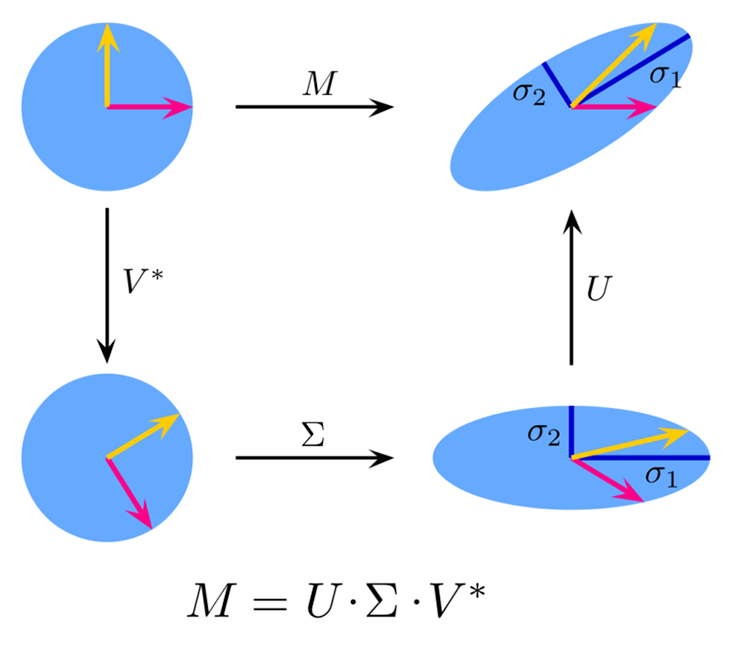
Theory:

image source: Wikipedia

Given a matrix  of dimensions  x , the singular value decomposition of   is given by:

where:

 is an  ×   orthogonal matrix (left singular vectors),

 is an  ×   diagonal matrix with singular values on the diagonal,

 is an   ×  orthogonal matrix (right singular vectors).

Truncated SVD keeps only the top k singular values and their corresponding vectors:

where:

 is an   ×   matrix,

 is a  ×    diagonal matrix,

 is an ×   matrix.

Implementation:

matrix CTruncatedSVD::fit_transform(matrix &X)
 {
  n_features = X.Cols();
  
   if (m_components>n_features)
     {
       printf("%s Number of dimensions K[%d] is supposed to be <= number of features %d",__FUNCTION__,m_components,n_features);
       this.m_components = (uint)n_features;
     }
   
    // Center the data (subtract mean)
    matrix X_centered = CDimensionReductionHelpers::subtract(X, X.Mean(0));
        
   // Compute the covariance matrix
    matrix cov_matrix = X_centered.Cov(false);
    
   // Perform SVD on the covariance matrix
    matrix U, Vt;
    vector Sigma;
    
    if (!X_centered.SVD(U,Vt,Sigma))
       Print(__FUNCTION__," Line ",__LINE__," Failed to calculate SVD Err=",GetLastError());    
        
    this.components_ = CDimensionReductionHelpers::Slice(Vt, this.m_components).Transpose();
    
    if (MQLInfoInteger(MQL_DEBUG))
      Print("components\n",CDimensionReductionHelpers::Slice(Vt, this.m_components),"\ncomponents_T\n",this.components_);
    
    this.explained_variance_ = MathPow(CDimensionReductionHelpers::Slice(Sigma, this.m_components), 2) / (X.Rows() - 1);
    
    return X_centered.MatMul(components_);
 }

There is a builtin-MQL5 method for calculating SVD of a matrix.

// Singular Value Decomposition.

bool matrix::SVD(
  matrix&  U,                   // unitary matrix 
  matrix&  V,                   // unitary matrix 
  vector&  singular_values      // singular values vector
   );

The fit_transform function does the following:

• It centers the data by subtracting the mean.
• It Computes the covariance matrix of the centered data(not important).
• It Performs SVD on the covariance matrix.
• It keeps the top k singular values and vectors.
• It constructs the reduced-dimensional representation of the original matrix.

This does work, But the real question is, How do we find the best number of k components for the data to be reduced?

Calculating Explained Variance Function

The function calculates the total variance by summing the squares of all singular values.

ulong CTruncatedSVD::_select_n_components(vector &singular_values)
 {
    double total_variance = MathPow(singular_values.Sum(), 2);
    
    vector explained_variance_ratio = MathPow(singular_values, 2).CumSum() / total_variance;
    
    if (MQLInfoInteger(MQL_DEBUG))
      Print(__FUNCTION__," Explained variance ratio ",explained_variance_ratio);
    
    vector k(explained_variance_ratio.Size());
    
    for (uint i=0; i<k.Size(); i++)
      k[i] = i+1;
    
    plt.ScatterCurvePlots("Explained variance plot",k,explained_variance_ratio,"variance","components","Variance");
    
   return explained_variance_ratio.ArgMax() + 1;  //Choose k for maximum explained variance
 }

The function takes an array of singular values (singular_values) as input. These singular values are obtained from the Singular Value Decomposition (SVD) of a matrix.

The function then selects the number of components (k) by finding the number of components k with the largest variance. This is achieved using this line of code:

explained_variance_ratio.ArgMax() + 1;

We need to modify our fit_transform function to make it capable of detecting the best number of components(when not given any number) to reduce the dimensions of the data and apply the number of components for the truncated SVD. 

matrix CTruncatedSVD::fit_transform(matrix &X)
 {
  n_features = X.Cols();
  
   if (m_components>n_features)
     {
       printf("%s Number of dimensions K[%d] is supposed to be <= number of features %d",__FUNCTION__,m_components,n_features);
       this.m_components = (uint)n_features;
     }
   
    // Center the data (subtract mean)
    matrix X_centered = CDimensionReductionHelpers::subtract(X, X.Mean(0));
        
   // Compute the covariance matrix
    matrix cov_matrix = X_centered.Cov(false);
    
   // Perform SVD on the covariance matrix
    matrix U, Vt;
    vector Sigma;
    
    if (!cov_matrix.SVD(U,Vt,Sigma))
       Print(__FUNCTION__," Line ",__LINE__," Failed to calculate SVD Err=",GetLastError());    
        
     if (m_components == 0)
       {
         m_components = (uint)this._select_n_components(Sigma);
         Print(__FUNCTION__," Best value of K = ",m_components);
       }
            
    this.components_ = CDimensionReductionHelpers::Slice(Vt, this.m_components).Transpose();
    
    if (MQLInfoInteger(MQL_DEBUG))
      Print("components\n",CDimensionReductionHelpers::Slice(Vt, this.m_components),"\ncomponents_T\n",this.components_);
    
    this.explained_variance_ = MathPow(CDimensionReductionHelpers::Slice(Sigma, this.m_components), 2) / (X.Rows() - 1);
    
    return X_centered.MatMul(components_);
 }

The default k value is now set to zero to allow this to happen effortlessly.

CTruncatedSVD::CTruncatedSVD(uint k=0)
:m_components(k)
 {
 
 }

Dimensionality Reduction using Truncated SVD

Now let's see how the data reduced in dimension by truncated SVD performs:

   truncated_svd = new CTruncatedSVD();
   
   data = truncated_svd.fit_transform(data);
   Print("Reduced matrix\n",data);

//--- 

   matrix train_x, test_x;
   vector train_y, test_y;
   
   data = matrix_utils.concatenate(data, target); //add the target variable to the dataset that is either normalized or not
   
   matrix_utils.TrainTestSplitMatrices(data, train_x, train_y, test_x, test_y, 0.7, 42);
     
   lr.fit(train_x, train_y, NORM_STANDARDIZATION); //training Linear regression model
   
   vector preds = lr.predict(train_x); //Predicting the training data
   
   Print("Train acc = ",metrics.r_squared(train_y, preds)); //Measuring the performance
  
   
   preds = lr.predict(test_x); //predicting the test data 
   
   Print("Test acc = ",metrics.r_squared(test_y, preds)); //measuring the performance

Outputs:

LH      0       20:13:41.385    dimension reduction test (EURUSD,H1)    CTruncatedSVD::_select_n_components Explained variance ratio [0.2399955100411572,0.3875113031818686,0.3903532427910986,0.3929609228375971,0.3932960517565894,0.3933072531960168,0.3933072531960282,0.3933072531960282,0.3933072531960282,0.3933072531960282]
EH      0       20:13:41.406    dimension reduction test (EURUSD,H1)    CTruncatedSVD::fit_transform Best value of K = 7
...
...
...
MR      0       20:13:41.407    dimension reduction test (EURUSD,H1)    Train acc = 0.8934645199970468
HP      0       20:13:41.407    dimension reduction test (EURUSD,H1)    Test acc = 0.8988671205298875

A stunning and stable performance 89.3% accuracy on training while 89.8% accuracy on testing. What about NMF?

What is NMF?

NMF stands for Non-Negative Matrix Factorization, and it is a dimensionality reduction technique that factorizes a matrix into two non-negative matrices. The goal of NMF is to represent the original matrix as the product of two lower-dimensional matrices, where all elements in the matrices are non-negative.

Given an input matrix X of dimensions m×n, NMF factorizes it into two matrices W and H such that:

Where:

 is an  ×    matrix, where k is the number of components or features.

 is a  ×    matrix.

Both  and  have non-negative entries, and this non-negativity constraint makes NMF particularly suitable for applications where the data is naturally non-negative, such as image data, text data, and spectrograms.

The factorization is achieved by minimizing the Frobenius norm of the difference between the original matrix  and its approximation  × . Mathematically, this can be expressed as:

 

where ​   denotes the Frobenius norm.

Implementation:

Transform Method

matrix CNMF::transform(matrix &X)
 {
  n_features = X.Cols();
  if (m_components>n_features)
     {
       printf("%s Number of dimensions K[%d] is supposed to be <= number of features %d",__FUNCTION__,m_components,n_features);
       this.m_components = (uint)n_features;
     }
     
  if (this.W.Rows()==0 || this.H.Rows()==0)
    {
      Print(__FUNCTION__," Model not fitted. Call fit method first.");
      matrix mat={};
      return mat;
    }
  
  return X.MatMul(this.H.Transpose());
 }

The transform function transforms new data X using the already fitted NMF components.

Fit Transform Method

matrix CNMF::fit_transform(matrix &X, uint k=2)
 {
  ulong m = X.Rows(), n = X.Cols();
  double best_frobenius_norm = DBL_MIN;
  
   m_components = m_components == 0 ? (uint)n : k;      
   
//--- Initialize Random values 

   this.W = CMatrixutils::Random(0,1, m, this.m_components, this.m_randseed);  
   this.H = CMatrixutils::Random(0,1,this.m_components, n, this.m_randseed);
   
//--- Update factors
      
   vector loss(this.m_max_iter);
    for (uint i=0; i<this.m_max_iter; i++)
      {
        // Update W
         this.W *= MathAbs((X.MatMul(this.H.Transpose())) / (this.W.MatMul(this.H.MatMul(this.H.Transpose()))+ 1e-10));
         
        // Update H
         this.H *= MathAbs((this.W.Transpose().MatMul(X)) / (this.W.Transpose().MatMul(this.W.MatMul(this.H))+ 1e-10));
         
         loss[i] = MathPow((X - W.MatMul(H)).Flat(1), 2);
                    
         // Calculate Frobenius norm of the difference
        double frobenius_norm = (X - W.MatMul(H)).Norm(MATRIX_NORM_FROBENIUS);

         if (MQLInfoInteger(MQL_DEBUG))
           printf("%s [%d/%d] Loss = %.5f frobenius norm %.5f",__FUNCTION__,i+1,m_max_iter,loss[i],frobenius_norm);
         
          // Check convergence
          if (frobenius_norm < this.m_tol)
              break;
      }
  
  return this.W.MatMul(this.H); 
 }

The fit_transform method performs NMF factorization on the input matrix X and returns the product of matrices W and H.

unlike the truncated SVD which we were able to write code to determine the number of components and apply it to itself, making using the truncated library easier, The NMF learning algorithm is quite different as it requires iterating over an n amount of iterations to find the best values for the algorithm, during the loop the number of k components must remain the same, that's why the fit_transform function takes the value of k components as one of its arguments.

We can get the best number of components for the Non-negative matrix factorization algorithm using the function select_best_components:

uint CNMF::select_best_components(matrix &X)
{
    uint best_components = 1;
    this.m_components = (uint)X.Cols();
    
    vector explained_ratio(X.Cols());    
    for (uint k = 1; k <= X.Cols(); k++)
    {
       // Calculate explained variance or other criterion 
       matrix X_reduced = fit_transform(X, k);
   
       // Calculate explained variance as the ratio of squared Frobenius norms
       double explained_variance = 1.0 - (X-X_reduced).Norm(MATRIX_NORM_FROBENIUS) / (X.Norm(MATRIX_NORM_FROBENIUS));
        
        if (MQLInfoInteger(MQL_DEBUG))
            printf("k %d Explained Var %.5f",k,explained_variance);
       
       explained_ratio[k-1] = explained_variance;       
    }
    return uint(explained_ratio.ArgMax()+1);
}

Due to the randomized nature of both Basic and Coefficient matrices, the results of the iterative multiplicative algorithm will be the random values too, so the outcome should be unpredictable unless the random state is set to some value greater than zero.

class CNMF
  {
protected:
   uint m_components;
   uint m_max_iter;
   int m_randseed;
   ulong n_features;
   matrix W; //Basic matrix
   matrix H; //coefficient matrix
   double m_tol; //loss tolerance
   
public:
                     CNMF(uint max_iter=100, double tol=1e-4, int random_state=-1);
                    ~CNMF(void);
                    
                    matrix fit_transform(matrix &X, uint k=2);
                    matrix transform(matrix &X);
                    uint select_best_components(matrix &X);
                    
  };

Dimensionality Reduction using NMF

Now let's see how the data reduced in dimension by Non-negative Matrix Factorization performs:

   nmf = new CNMF(30);
   
   data = nmf.fit_transform(data, 10);
   Print("Reduced matrix\n",data);

//--- 

   matrix train_x, test_x;
   vector train_y, test_y;
   
   data = matrix_utils.concatenate(data, target); //add the target variable to the dataset that is either normalized or not
      
   matrix_utils.TrainTestSplitMatrices(data, train_x, train_y, test_x, test_y, 0.7, 42);
      
   lr.fit(train_x, train_y, NORM_STANDARDIZATION); //training Linear regression model
   
   vector preds = lr.predict(train_x); //Predicting the training data
   
   Print("Train acc = ",metrics.r_squared(train_y, preds)); //Measuring the performance
   
   preds = lr.predict(test_x); //predicting the test data 
   
   Print("Test acc = ",metrics.r_squared(test_y, preds)); //measuring the performance
   

Outcomes:

DG      0       11:51:07.197    dimension reduction test (EURUSD,H1)    Best k components = 10
LG      0       11:51:07.197    dimension reduction test (EURUSD,H1)    CNMF::fit_transform [1/30] Loss = 187.40949 frobenius norm 141.12462
EG      0       11:51:07.198    dimension reduction test (EURUSD,H1)    CNMF::fit_transform [2/30] Loss = 106.49597 frobenius norm 130.94039
KS      0       11:51:07.198    dimension reduction test (EURUSD,H1)    CNMF::fit_transform [3/30] Loss = 84.38553 frobenius norm 125.05413
OS      0       11:51:07.198    dimension reduction test (EURUSD,H1)    CNMF::fit_transform [4/30] Loss = 67.07345 frobenius norm 118.96900
OR      0       11:51:07.198    dimension reduction test (EURUSD,H1)    CNMF::fit_transform [5/30] Loss = 52.50290 frobenius norm 112.46587
LR      0       11:51:07.198    dimension reduction test (EURUSD,H1)    CNMF::fit_transform [6/30] Loss = 40.14937 frobenius norm 105.48081
RR      0       11:51:07.198    dimension reduction test (EURUSD,H1)    CNMF::fit_transform [7/30] Loss = 29.79307 frobenius norm 98.11626
IR      0       11:51:07.198    dimension reduction test (EURUSD,H1)    CNMF::fit_transform [8/30] Loss = 21.32224 frobenius norm 90.63011
NS      0       11:51:07.198    dimension reduction test (EURUSD,H1)    CNMF::fit_transform [9/30] Loss = 14.63453 frobenius norm 83.36462
HL      0       11:51:07.199    dimension reduction test (EURUSD,H1)    CNMF::fit_transform [10/30] Loss = 9.58168 frobenius norm 76.62838
NL      0       11:51:07.199    dimension reduction test (EURUSD,H1)    CNMF::fit_transform [11/30] Loss = 5.95040 frobenius norm 70.60136
DM      0       11:51:07.199    dimension reduction test (EURUSD,H1)    CNMF::fit_transform [12/30] Loss = 3.47775 frobenius norm 65.31931
LM      0       11:51:07.199    dimension reduction test (EURUSD,H1)    CNMF::fit_transform [13/30] Loss = 1.88772 frobenius norm 60.72185
EN      0       11:51:07.199    dimension reduction test (EURUSD,H1)    CNMF::fit_transform [14/30] Loss = 0.92792 frobenius norm 56.71242
RO      0       11:51:07.199    dimension reduction test (EURUSD,H1)    CNMF::fit_transform [15/30] Loss = 0.39182 frobenius norm 53.19791
NO      0       11:51:07.199    dimension reduction test (EURUSD,H1)    CNMF::fit_transform [16/30] Loss = 0.12468 frobenius norm 50.10411
NH      0       11:51:07.199    dimension reduction test (EURUSD,H1)    CNMF::fit_transform [17/30] Loss = 0.01834 frobenius norm 47.37568
KI      0       11:51:07.199    dimension reduction test (EURUSD,H1)    CNMF::fit_transform [18/30] Loss = 0.00129 frobenius norm 44.96962
KI      0       11:51:07.200    dimension reduction test (EURUSD,H1)    CNMF::fit_transform [19/30] Loss = 0.02849 frobenius norm 42.84850
MJ      0       11:51:07.200    dimension reduction test (EURUSD,H1)    CNMF::fit_transform [20/30] Loss = 0.07289 frobenius norm 40.97668
RJ      0       11:51:07.200    dimension reduction test (EURUSD,H1)    CNMF::fit_transform [21/30] Loss = 0.11920 frobenius norm 39.31975
QK      0       11:51:07.200    dimension reduction test (EURUSD,H1)    CNMF::fit_transform [22/30] Loss = 0.15954 frobenius norm 37.84549
FD      0       11:51:07.200    dimension reduction test (EURUSD,H1)    CNMF::fit_transform [23/30] Loss = 0.19054 frobenius norm 36.52515
RD      0       11:51:07.200    dimension reduction test (EURUSD,H1)    CNMF::fit_transform [24/30] Loss = 0.21142 frobenius norm 35.33409
KE      0       11:51:07.200    dimension reduction test (EURUSD,H1)    CNMF::fit_transform [25/30] Loss = 0.22283 frobenius norm 34.25183
PF      0       11:51:07.200    dimension reduction test (EURUSD,H1)    CNMF::fit_transform [26/30] Loss = 0.22607 frobenius norm 33.26170
GF      0       11:51:07.200    dimension reduction test (EURUSD,H1)    CNMF::fit_transform [27/30] Loss = 0.22268 frobenius norm 32.35028
NG      0       11:51:07.201    dimension reduction test (EURUSD,H1)    CNMF::fit_transform [28/30] Loss = 0.21417 frobenius norm 31.50679
CG      0       11:51:07.201    dimension reduction test (EURUSD,H1)    CNMF::fit_transform [29/30] Loss = 0.20196 frobenius norm 30.72260
CP      0       11:51:07.201    dimension reduction test (EURUSD,H1)    CNMF::fit_transform [30/30] Loss = 0.18724 frobenius norm 29.99074
...
...
FS      0       11:51:07.201    dimension reduction test (EURUSD,H1)    Train acc = 0.604329883526616
IR      0       11:51:07.202    dimension reduction test (EURUSD,H1)    Test acc = 0.5115967009955317

The function select_best_components found that the best number of components was 10, the same as the number of columns in the dataset we gave it, It is fair to say that the accuracy of the data resulted from NMF when applied to the linear regression model produced average results of  61% during training and 51% during testing. Before we conclude that TruncatedSVD is a clear winner in this situation However, we need to acknowledge the fact that Non-negative Matrix Factorization(NMF) requires much programming to make it work. When implemented properly and with a better learning algorithm such as Stochastic Gradient Descent(SGD) or any other smart learning algorithm, it can produce a better dataset but for the basic implementations on both algorithms! Truncated SVD won(on paper though)

Let's see how both perform in the big data:

Let's apply the entire data to our algorithms and measure how would they fare in the entire dataset, This will gives us a clue as to which method should be applied to get the best compressed data for our linear regression model.

Truncated SVD Versus NMF, The Battle

This time no data was filtered, we went all in with all the indicators applied for the truncated SVD.

void TrainTestLR(int start_bar=1)
 {
   string names;
   matrix data = indicators.GetAllBuffers(names, start_bar, buffer_size);   
   
//--- Getting close values

   MqlRates rates[];
   ArraySetAsSeries(rates, true);
   CopyRates(Symbol(), PERIOD_CURRENT, start_bar, buffer_size, rates);
   
   double targ_Arr[];
   ArrayResize(targ_Arr, buffer_size);
   
   for (int i=0; i<buffer_size; i++)
     targ_Arr[i] = rates[i].close;
   
   vector target = matrix_utils.ArrayToVector(targ_Arr);
      
//--- Dimension reduction process 
   
   switch(dimension_redux)
     {
      case  NMF:
        {
          nmf = new CNMF(nmf_iterations);
         
          uint k = nmf.select_best_components(data);
          //Print("Best k components = ",k);
          data = nmf.fit_transform(data, k);    
        }
        break;
      case TRUNC_SVD:
      
         truncated_svd = new CTruncatedSVD();
         data = truncated_svd.fit_transform(data);  
         
        break;
      case None:
        break;
     }
     
//---

  Print(EnumToString(dimension_redux)," Reduced matrix[",data.Rows(),"x",data.Cols(),"]\n",data);
  
//--- 

   matrix train_x, test_x;
   vector train_y, test_y;
   
   data = matrix_utils.concatenate(data, target); //add the target variable to the dimension reduced data
      
   matrix_utils.TrainTestSplitMatrices(data, train_x, train_y, test_x, test_y, 0.7, 42);
      
   lr.fit(train_x, train_y, NORM_STANDARDIZATION); //training Linear regression model
   
   vector preds = lr.predict(train_x); //Predicting the training data
   
   Print("Train acc = ",metrics.r_squared(train_y, preds)); //Measuring the performance
   
   preds = lr.predict(test_x); //predicting the test data 
   
   Print("Test acc = ",metrics.r_squared(test_y, preds)); //measuring the performance

 }

In the inputs section TRUNC_SVD which stands for Truncated SVD was selected:

The results were outstanding as expected for truncated SVD. The data was compressed into 11 useful components at the pivotal point of the graph below

Outputs:

KI      0       13:35:07.262    dimension reduction test (EURUSD,H1)    [56x56] Covariance
HS      0       13:35:07.262    dimension reduction test (EURUSD,H1)    [[1.659883222775595e-05,0.03248108864728622,0.002260592127494286,0.002331226815118805,0.0473802958063898,0.009411152185446843,-0.0007144995075063451,1.553267567351765e-05,1.94117385500497e-05,1.165361279698562e-05,1.596183979153003e-05,1.56892102141789e-05,1.565786314082391e-05,1.750827764889262e-05,1.568797564383075e-05,1.542116504856457e-05,1.305965012072059e-05,1.184306318548672e-05,0,1.578309112710041e-05,1.620880130984106e-05,3.200794587841053e-07,1.541769717649654e-05,1.582152318930163e-05,5.986572608120619e-07,-7.489818958341503e-07,-1.347949386573036e-07,1.358668593395908,-0.0551110816439555,7.279528408421348e-05,-0.0001838813666139953,5.310112938097826e-07,6.759105066381161e-07,1.755806692036581e-05,-1.448992128283333e-07,0.003656398187537544,-2.423948560741599e-05,1.65581437719033e-05,-0.01251289868226832,-0.007951606834421109,8.315844054428887e-08,-0.02211745766272421,58.3452835083685,-0.004138620879652527,115.0719348800515,0.7113815226449098,-3.467421230325816e-07,1.456828920113124e-05,1.536603660063518e-05,1.576222466715787e-05,6.85495465028602e-07,0,0,1.264184887739262e-06,-8.035590653384948e-05,-6.948836688267333e-07]
DG      0       13:35:07.262    dimension reduction test (EURUSD,H1)     [0.03248108864728622,197.2946284096305,47.5593359902222,-70.84984591299812,113.00968468357,80.50832448214619,-85.73100643892406,0.01887146397983594,0.03089371802428824,0.006849209935383654,0.03467670330041064,0.02416916876582018,0.02412087871833598,0.0345064443900023,0.03070601018237932,0.02036445858890056,0.009641324468627534,0.006973716378187099,0,0.02839705603036633,0.02546230398502955,0.000344615196142723,0.04030780408653764,0.02543558488321825,0.0003508232190957864,0.00918131954773614,0.009950700238139187,18501.50888551419,578.0227911644578,1.963532857377992,7.661630153435527,0.006966837168084083,0.004556433245004339,2.562261625497797,0.002410403923079745,118.382177007498,1.555763207775421,1.620640369180333,97.88352837129584,116.7606184094667,0.0006817870698682788,163.5401896749969,108055.4673427991,140.7005993870342,173684.2642498043,3567.96895955429,0.0026091195479834,0.01088219157686945,0.01632411390047346,0.02372834986595739,0.02071124643451263,0,0,0.003953688163493562,-1.360529605248643,-0.04542261766857811]
IL      0       13:35:07.262    dimension reduction test (EURUSD,H1)     [0.002260592127494286,47.5593359902222,39.19958980374253,-35.49971367926001,7.967839162735706,33.38887983973432,-33.90876164339727,-0.001453063639065681,-0.000297822858867019,-0.002608304419264346,0.002816269112655834,-0.0006711791217058063,-0.0006698381044796457,0.002120545460717355,0.002300146098203005,0.0001826452994732207,-0.0003768483866125172,-0.002445364564315893,0,0.0003665645439668078,-0.003400376924338417,-1.141907378821958e-06,0.006568498854351883,0.0006581929826678372,-0.0005502523415197902,0.00579179204268979,0.006348707171855972,7967.929705662135,452.5996105540225,0.7520153701277594,4.211592829265125,0.001461149548206051,0.0001367863805269901,0.8802824558924612,0.001324363167679062,50.70542641656378,0.6826775813408293,0.5131585731076505,116.3828090044126,97.64469627257866,5.244397974811099e-05,113.6246589165999,13312.60086575102,66.02007474397942,15745.06353439358,3879.735235353455,0.002648988695504766,-0.00244724050922883,-0.00263645588222185,-0.001438073133818628,0.005654239425742305,0,0,-0.000119694862927093,-0.3588916052856576,-0.1059287487094797]
EM      0       13:35:07.262    dimension reduction test (EURUSD,H1)     [0.002331226815118805,-70.84984591299812,-35.49971367926001,60.69058251292376,1.049456584665883,-42.35184208285295,60.90812761343581,0.008675881760275542,0.008620685402656748,0.008731078117894331,-0.000667294720674837,0.005845080481159768,0.005833401998679988,0.002539790385479495,0.001675796458760079,0.00792229604709134,0.01072137357191657,0.01189054942647922,0,0.003518070782066417,0.00809138574827074,0.0002045106345618818,-0.005848319055742076,0.005549764528898804,0.00103946798619902,-0.008604821519805591,-0.007960056731330659,-10509.62154107038,-607.7276555152829,-1.225906326607001,-5.179537786920108,-0.003656220590983723,-0.001714862736227047,-1.657652278786164,-0.001941357854756676,-80.61630801951124,-1.158614351229071,-1.010395372975761,-137.5151461158883,-129.0146405010356,…]
DK      0       13:35:07.264    dimension reduction test (EURUSD,H1)    CTruncatedSVD::_select_n_components Explained variance ratio [0.9718079496976207,0.971876424055512,0.9718966593387935,0.971898669685807,0.9718986697080317,0.9718986697081728,0.9718986697082533,0.9718986697082695,0.9718986697082731,0.9718986697082754,0.9718986697082757,0.9718986697082757,0.9718986697082757,0.9718986697082757,0.9718986697082757,0.9718986697082757,0.9718986697082757,0.9718986697082757,0.9718986697082757,0.9718986697082757,0.9718986697082757,0.9718986697082757,0.9718986697082757,0.9718986697082757,0.9718986697082757,0.9718986697082757,0.9718986697082757,0.9718986697082757,0.9718986697082757,0.9718986697082757,0.9718986697082757,0.9718986697082757,0.9718986697082757,0.9718986697082757,0.9718986697082757,0.9718986697082757,0.9718986697082757,0.9718986697082757,0.9718986697082757,0.9718986697082757,0.9718986697082757,0.9718986697082757,0.9718986697082757,0.9718986697082757,0.9718986697082757,0.9718986697082757,0.9718986697082757,0.9718986697082757,0.9718986697082757,0.9718986697082757,0.9718986697082757,0.9718986697082757,0.9718986697082757,0.9718986697082757,0.9718986697082757,0.9718986697082757]
JJ      0       13:35:07.282    dimension reduction test (EURUSD,H1)    CTruncatedSVD::fit_transform Best value of K = 11
FE      0       13:35:07.282    dimension reduction test (EURUSD,H1)    components
GP      0       13:35:07.282    dimension reduction test (EURUSD,H1)    [[1.187125882554785e-07,1.707109381366902e-07,-2.162493440707256e-08,-3.212808990986057e-07,1.871672229653978e-07,-1.333159242305641e-05,-1.709658791626167e-05,5.106786021196193e-05,2.160157948893384e-05,-1.302989528292599e-06,4.973487699412528e-06,2.354866764130305e-06,0.0001127065022780296,-0.0001141032171988836,-7.674973628685988e-05,4.318893830956814e-06,-8.017085790662858e-05,1.258581118770149e-05,0.001793756756130711,0.0002550931459979332,0.0005154637372606566,0.001801147973070216,0.0001081777898713252,0.1803191282351903,-0.0971245889819613,0.1677985300894154,0.1116153850447159,0.6136670152098842,0.022810600805461,-0.4096528016535661,-0.04163009420605639,-6.077467743293966e-06,-0.01526638316446551,-0.5288520838909793,-0.03965140358106178,-0.1758179670991415,-0.003645717072725773,-0.0587633049540756,0.004124498383003558,-0.1172419838852104,0.06762215235985558,-0.04328191674666172,0.002573659612267772,0.003811049362514162,-0.0659455961610354,-0.02792883463906511,0.008647163802477509,-0.05514899696636823,0.008017364204121686,2.516946811168054e-06,-0.1623798112317545,6.339565837779877e-07,-9.103773865679859e-08,0,0,0]
CH      0       13:35:07.282    dimension reduction test (EURUSD,H1)     [0.000187434605818864,0.002812180913638008,0.000925532096115269,0.003073325320378009,0.009404433538995808,-0.1105512584754667,-0.2590049789665196,0.4726584971639716,0.1447383637844528,-0.05374370025421956,-0.752572111353205,0.04852191253671465,-0.1154729372340165,-0.2700032006603445,0.1267147455792905,-0.04806661586591762,-0.0004106947202907203,-0.001517506503982104,-0.003502569576390078,-0.002616630851275089,-0.0003258690084512006,-1.313122566421376e-05,-0.0009386837340425192,7.909925585103072e-05,-7.798476572374581e-05,-8.126463184191059e-05,5.556082790448295e-05,-2.687039190421141e-05,-6.540787996573879e-06,1.330764390715927e-05,-4.491635420079414e-05,-8.144156726118825e-06,-8.508538790002811e-07,5.307068574641107e-05,8.482440778162809e-06,-2.9724306932086e-05,2.843845070244019e-05,1.220433778827776e-05,4.206331251218703e-06,1.256512854012554e-05,7.365925693883173e-06,-1.116338606511276e-05,-2.071419560390051e-06,-3.218285979262829e-06,-1.138651025910271e-05,-7.728111919788928e-06,-4.653652137908648e-06,-9.580813709785919e-06,-1.028740118967147e-05,-6.979591632948435e-06,8.116615752437345e-06,1.763108270729631e-06,-4.348070304093866e-07,0,0,0]
JR      0       13:35:07.282    dimension reduction test (EURUSD,H1)     [1.848792316776081e-05,0.0008588118715707877,0.001008311173244842,0.002376194713912998,0.03118554398340165,0.07889519945845663,-0.07568381470451135,0.0286506682781276,-0.09873220604411656,-0.09161678196011247,-0.06574722506621368,-0.8477734032486133,-0.2533539865405071,0.01738574140899809,-0.2520128661222155,0.338533576002899,0.03018091859501061,0.03802772499047165,-0.001646103636389454,-0.00230341248842314,0.007310099460075021,-0.006012419384786831,-0.001413152018214914,2.142238614111051e-05,2.944210407515316e-05,-6.521097350129076e-05,4.95794487446122e-05,-8.706533732190571e-06,3.322659358695792e-05,-8.146689287415223e-07,7.338661273889888e-06,6.605547217087068e-06,9.447199984574336e-06,-5.17902002055696e-05,2.513872334761899e-06,-2.256988836110105e-05,-1.911456753589991e-05,-3.264899090321399e-05,-5.800966034108816e-06,1.84157480007614e-05,5.356185659483905e-06,-1.722849771456492e-05,1.407694486288703e-05,-7.853816348797691e-06,-1.555432680785718e-05,1.323568644672602e-05,-6.760913172750632e-06,-1.302135272406512e-05,-3.211793238456227e-06,5.802687671843603e-07,-4.280158053673846e-06,1.549960937140237e-06,-4.919157307518426e-07,0,0,0]
ND      0       13:35:07.282    dimension reduction test (EURUSD,H1)     [4.113935038265459e-05,-0.00163116425762962,-0.0006793200544509552,-0.002550542034446345,-0.0360619764220519,-0.05083503039040507,0.1457232134777539,-0.1319534223026893,-0.1000465688426969,0.03066773678926198,0.211126338548004,0.02610057183969087,-0.4621259104920466,-0.5881871797892803,0.5329599008633419,0.2326293789423069,-0.004192622153062945,-0.05839467173045784,0.002320319216461524,0.007699098543144081,-0.007658991162669676,-0.003166005488782055,-0.002283364895801648,0.0001978857108759482,9.652410400630472e-05,5.391765247424044e-05,-2.114027852314159e-05,-3.571496353187668e-06,6.919610375993553e-06,-2.388732546126286e-05,-1.795211964869842e-05,-4.375012411627235e-05,-6.279526099805299e-05,2.71361750709131e-06,-2.519904126359203e-05,-3.154274545518064e-05,-4.95034356619025e-05,4.982607182957078e-05,2.91223664932767e-05,7.266298957499022e-06,-5.27732883601878e-0…]
QD      0       13:35:07.283    dimension reduction test (EURUSD,H1)    TRUNC_SVD Reduced matrix[100x11]
FJ      0       13:35:07.283    dimension reduction test (EURUSD,H1)    [[3032.510155721446,0.6797958296629614,0.3147476036369294,-1.879105115460979,2.342311343896795,-1.444862488231156,1.72748820545895,9003.45453268309,6583.0037062413,11248.15180107277,7664.89601210886]
QF      0       13:35:07.283    dimension reduction test (EURUSD,H1)     [2613.746957390415,0.8994353272147151,0.2278876639409569,-1.833173521667439,2.422820504229084,-1.194855144516288,1.619766862896731,8730.428168136412,6321.389560496657,10843.26327739175,7319.502533761807]
PE      0       13:35:07.283    dimension reduction test (EURUSD,H1)     [2290.391536977857,0.8379176898463352,0.123448650655239,-1.79572777997295,2.553555290053082,-1.261720012039457,1.872612496522998,9359.431555011421,6628.023623123124,11573.90347441899,7725.564567458286]
MG      0       13:35:07.283    dimension reduction test (EURUSD,H1)     [1793.638587775052,0.8840827856664026,-0.009259140368535656,-1.812929578463889,2.752934946133839,-1.194132624145421,2.137669035967074,10045.24774931484,6958.660329797975,12319.85906895874,8090.242616080116]
IG      0       13:35:07.283    dimension reduction test (EURUSD,H1)     [1067.248927502046,0.9361386848947133,0.2824462001532311,-2.094258230827017,2.302295904768048,-0.9859566963069195,1.849760818059724,8852.426567434784,5936.081092995532,10850.91447636461,7048.244994007338]
NK      0       13:35:07.283    dimension reduction test (EURUSD,H1)     [875.831228770905,1.10630868463423,0.3875078994082357,-2.07189694520072,2.003365098290179,-0.8110375102176066,1.363090061871958,7086.981018896034,4689.12320342304,8755.082428498208,5718.774787652458]
GK      0       13:35:07.283    dimension reduction test (EURUSD,H1)     [750.5105412678478,1.58876151742295,0.4277968820488219,-2.495434492237099,2.546292376170158,-0.5828893757361142,1.468026541982692,8457.543559890122,5579.75159746014,10352.91442474459,6691.476688344664]
EK      0       13:35:07.283    dimension reduction test (EURUSD,H1)     [1028.864261893481,1.737564309663063,0.6859148896559381,-2.576387294650619,2.22158096752311,-0.3483142589026745,0.9424367352835165,7447.770506698205,5028.271311988544,9145.898159310427,5970.749558054185]
MJ      0       13:35:07.283    dimension reduction test (EURUSD,H1)     [1315.206321750198,1.599230058650526,1.006274380327883,-2.7208483981554,1.702262719567507,-0.3336344655640055,0.5851633683692923,6123.681144041253,4208.879528858515,7625.280231352584,5091.190116446857]
PI      0       13:35:07.283    dimension reduction test (EURUSD,H1)     [1040.359603039049,2.015870643904685,1.297584348509677,-3.422661750068991,2.051984203691556,-0.1752179554187868,0.625382499042994,7446.846626605789,4973.286352001192,9200.911151239434,6040.469516939555]
MJ      0       13:35:07.283    dimension reduction test (EURUSD,H1)     [2056.827104147074,0.6969653180001977,0.5026500071613408,-1.539526411095017,1.333168361525386,-1.205142789226661,0.6457357287148752,4362.936467349854,3118.514061447938,5739.541487386377,4094.4444510553]
KI      0       13:35:07.283    dimension reduction test (EURUSD,H1)     [2595.720157415741,0.5163475309230526,0.7707831677360033,-1.609464385287863,0.6391376890497206,-1.091660522613616,0.2434028653397404,2245.471581325966,1932.755290423922,3219.551710692477,2600.234934440349]
FJ      0       13:35:07.283    dimension reduction test (EURUSD,H1)     [2000.813854424802,-0.1645196557230545,0.0271698872028618,-1.136148599089293,1.199419424319289,-1.596267278271581,1.616290624329739,4340.908808342276,3155.426978423527,5643.263654816839,4006.305187235153]
GN      0       13:35:07.283    dimension reduction test (EURUSD,H1)     [714.201770611258,0.3322650152566928,-0.128924730742915,-1.497052055771412,1.889908667964611,-1.18328154703613,2.040965402442796,6411.664479403819,4214.549479233159,7917.864243044486,5153.2871400763]
PN      0       13:35:07.283    dimension reduction test (EURUSD,H1)     [676.7845833423586,0.1119963611895549,-0.4614956061196153,-0.7783442013329294,1.680735950870798,-1.110059082233565,1.926793017792492,5379.745050208609,3591.380424598063,6620.153862582291,4307.434978894435]
GL      0       13:35:07.283    dimension reduction test (EURUSD,H1)     [766.9657214036708,0.3283061830008722,-0.3885600107901345,-1.031650548898253,1.912288786544761,-1.036499883901753,2.01321049032323,6312.725946828255,4249.957068368147,7723.98867795246,5012.0279192467]
LN      0       13:35:07.283    dimension reduction test (EURUSD,H1)     [1272.697206108888,-0.3546159778199272,-0.7521309963906442,-0.1806331494361637,1.527697751794935,-1.486437217294949,2.136800392269752,5073.89079322631,3559.651506707118,6317.965379534476,4229.397904810504]
RM      0       13:35:07.283    dimension reduction test (EURUSD,H1)     [1869.479624807111,-0.0175694426730242,-0.7678796689175619,-0.2643173159395689,1.862033543014759,-1.44967470564508,2.028361828380722,5639.625182760593,4124.447639836587,7033.466549718048,4777.911629224665]
GN      0       13:35:07.283    dimension reduction test (EURUSD,H1)     [1936.02506453734,0.0845940044872068,-0.8282752540396139,-0.2824304083282199,1.982789807497455,-1.350085518779075,2.085883725566998,5911.195073473721,4372.189044548059,7316.534104301676,4945.624347822407]
CR      0       13:35:07.283    dimension reduction test (EURUSD,H1)     [1844.238763352675,-0.4606751585910102,-1.187448989349241,0.2320045292554417,1.900279565663612,-1.62110507361112,2.534343850099422,5907.730651516376,4364.59879103891,7282.962351393813,4893.24121551531]
ER      0       13:35:07.283    dimension reduction test (EURUSD,H1)     [1716.303347926322,-0.2450617860724134,-0.9482067759826802,-0.03979477150523128,1.79416546386642,-1.453641927846228,2.284520496569503,5710.722665215339,4183.828568899002,7048.670774203967,4734.907606214866…]
GP      0       13:35:07.283    dimension reduction test (EURUSD,H1)    Train acc = 0.8087284075835584
ER      0       13:35:07.283    dimension reduction test (EURUSD,H1)    Test acc = 0.7286157353628964

80% accurate on the training sample while being 72% accurate on the testing sample.

Non-negative Matrix Factorization(NMF)

On the other hand, the NMF was unable to produce anything of value as anything resulting from it was a nan value, at this point, it is no longer a competitor. 

LK      0       13:43:09.997    dimension reduction test (EURUSD,H1)    CNMF::fit_transform [1/100] Loss = nan frobenius norm nan
II      0       13:43:09.997    dimension reduction test (EURUSD,H1)    CNMF::fit_transform [2/100] Loss = nan frobenius norm nan
FG      0       13:43:09.997    dimension reduction test (EURUSD,H1)    CNMF::fit_transform [3/100] Loss = nan frobenius norm nan
KF      0       13:43:09.997    dimension reduction test (EURUSD,H1)    CNMF::fit_transform [4/100] Loss = nan frobenius norm nan
PD      0       13:43:09.997    dimension reduction test (EURUSD,H1)    CNMF::fit_transform [5/100] Loss = nan frobenius norm nan
PR      0       13:43:09.998    dimension reduction test (EURUSD,H1)    CNMF::fit_transform [6/100] Loss = nan frobenius norm nan
KP      0       13:43:09.998    dimension reduction test (EURUSD,H1)    CNMF::fit_transform [7/100] Loss = nan frobenius norm nan
NO      0       13:43:09.998    dimension reduction test (EURUSD,H1)    CNMF::fit_transform [8/100] Loss = nan frobenius norm nan
QM      0       13:43:09.998    dimension reduction test (EURUSD,H1)    CNMF::fit_transform [9/100] Loss = nan frobenius norm nan
MH      0       13:43:09.998    dimension reduction test (EURUSD,H1)    CNMF::fit_transform [10/100] Loss = nan frobenius norm nan
....
....
LM      0       13:43:10.006    dimension reduction test (EURUSD,H1)    CNMF::fit_transform [97/100] Loss = nan frobenius norm nan
OO      0       13:43:10.006    dimension reduction test (EURUSD,H1)    CNMF::fit_transform [98/100] Loss = nan frobenius norm nan
NI      0       13:43:10.006    dimension reduction test (EURUSD,H1)    CNMF::fit_transform [99/100] Loss = nan frobenius norm nan
CI      0       13:43:10.006    dimension reduction test (EURUSD,H1)    CNMF::fit_transform [100/100] Loss = nan frobenius norm nan
MI      0       13:43:10.008    dimension reduction test (EURUSD,H1)    NMF Reduced matrix[100x56]
FN      0       13:43:10.008    dimension reduction test (EURUSD,H1)    [[nan,nan,nan,nan,nan,nan,nan,nan,nan,nan,nan,nan,nan,nan,nan,nan,nan,nan,nan,nan,nan,nan,nan,nan,nan,nan,nan,nan,nan,nan,nan,nan,nan,nan,nan,nan,nan,nan,nan,nan,nan,nan,nan,nan,nan,nan,nan,nan,nan,nan,nan,nan,nan,nan,nan,nan]
EF      0       13:43:10.008    dimension reduction test (EURUSD,H1)     [nan,nan,nan,nan,nan,nan,nan,nan,nan,nan,nan,nan,nan,nan,nan,nan,nan,nan,nan,nan,nan,nan,nan,nan,nan,nan,nan,nan,nan,nan,nan,nan,nan,nan,nan,nan,nan,nan,nan,nan,nan,nan,nan,nan,nan,nan,nan,nan,nan,nan,nan,nan,nan,nan,nan,nan]
GK      0       13:43:10.008    dimension reduction test (EURUSD,H1)     [nan,nan,nan,nan,nan,nan,nan,nan,nan,nan,nan,nan,nan,nan,nan,nan,nan,nan,nan,nan,nan,nan,nan,nan,nan,nan,nan,nan,nan,nan,nan,nan,nan,nan,nan,nan,nan,nan,nan,nan,nan,nan,nan,nan,nan,nan,nan,nan,nan,nan,nan,nan,nan,nan,nan,nan]
QO      0       13:43:10.008    dimension reduction test (EURUSD,H1)     [nan,nan,nan,nan,nan,nan,nan,nan,nan,nan,nan,nan,nan,nan,nan,nan,nan,nan,nan,nan,nan,nan,nan,nan,nan,nan,nan,nan,nan,nan,nan,nan,nan,nan,nan,nan,nan,nan,nan,nan,nan,nan,nan,nan,nan,nan,nan,nan,nan,nan,nan,nan,nan,nan,nan,nan]
CL      0       13:43:10.008    dimension reduction test (EURUSD,H1)     
...
....
EO      0       13:43:10.008    dimension reduction test (EURUSD,H1)     [nan,nan,nan,nan,nan,nan,nan,nan,nan,nan,nan,nan,nan,nan,nan,nan,nan,nan,nan,nan,nan,nan,nan,nan,nan,nan,nan,nan,nan,nan,nan,nan,nan,nan,nan,nan,nan,nan,nan,nan,nan,nan,nan,nan,nan,nan,nan,nan,nan,nan,nan,nan,nan,nan,nan,nan…]
EL      0       13:43:10.010    dimension reduction test (EURUSD,H1)    Train acc = nan
GJ      0       13:43:10.010    dimension reduction test (EURUSD,H1)    Test acc = nan

Let's try to build a linear regression model without truncated SVD, let's just apply the entire data to it and observe how its performance.

GM      0       13:53:03.686    dimension reduction test (EURUSD,H1)    None Reduced matrix[100x56]
MG      0       13:53:03.686    dimension reduction test (EURUSD,H1)    [[1.099900334222465,28.09636760954466,23.62682944559725,20.05254468697356,24.9034642580335,25.12500390358301,19.04617822178984,1.098553499999958,1.102834674021181,1.094272325978734,1.100734208567449,1.100855469999989,1.098655958571417,1.100133799959087,1.09983,1.097395,1.0950725,1.094895,1.10265,1.100030000000004,1.09944087984,0.03659425270713104,1.100626095746222,1.098825209694279,0.001265714285714323,1.705459946510501e-05,0.0009170545994650059,1655.083284093067,24.54629344924639,0.4388379204892836,0.1040346153847089,0.001226921314023466,0.0012463900886654,100.1775875415509,-1.946877464193406e-05,63.53135141907871,0.1040413928121892,0.1171616554839711,43.66576819407196,56.26437671196908,0.000170982627085528,-39.78494623655773,-2966278.270646845,59.66122501825306,-426422,2459,-0.0002127529411762598,1.096805768175659,1.098423909197834,1.099767192241293,0.00330055882353042,1.797693134862316e+308,1.797693134862316e+308,0.001618141022174502,0,0.03660024400162265]
DH      0       13:53:03.687    dimension reduction test (EURUSD,H1)     [1.099895090784212,25.44125240854614,20.47658551951762,17.37887206204375,24.10764337690182,24.31185250851098,18.42976333679036,1.098807999999958,1.102730359493936,1.09488564050598,1.100648597660533,1.100904089999989,1.09870448142856,1.100085345856641,1.09983,1.097395,1.0949775,1.09511,1.10237,1.100145000000004,1.09954,0.03659633771631932,1.100539015261062,1.098860393123325,0.001167857142857174,0.000137475370969975,0.0006774753709699599,1151.094538712408,-2.654176423441059,0.4388379204892836,0.1582615384614039,0.001148578761165142,0.001262448000841409,100.0618688017469,-0.0001138692396762668,61.34588689321424,0.1137518684603838,0.1082289779011129,39.39899833055219,47.44710420521373,0.000170240277350424,-32.25806451612595,-2966207.715091289,53.52331983100873,-424517,1905,-0.0003920588235292355,1.097045324469839,1.098718420548105,1.099909753793035,0.003008823529412785,1.797693134862316e+308,1.797693134862316e+308,0.001673096078265379,0,0.0283464566929126]
LG      0       13:53:03.687    dimension reduction test (EURUSD,H1)     [1.099896454740888,23.0468607955726,17.74637411691527,20.61724467599245,23.13044479515374,23.58127757886977,19.12803587728702,1.099111999999958,1.102374285088665,1.095849714911251,1.100636052620929,1.100962719999989,1.098762994285703,1.100079584777576,1.09983,1.097395,1.0949025,1.09511,1.10224,1.100252000000004,1.10126,0.03659849012444888,1.10032475011848,1.098869304036258,0.001062857142857168,-6.787825345444531e-05,0.0004021217465455251,385.6853260090575,21.57900929644156,0.4735973597359621,0.1358284615387142,0.001095648513071756,0.001261794377734486,100.0745976729165,-0.00016614586466273,63.02688593246703,0.1054308010829696,0.1073759442661703,21.12676056338241,34.73050902933566,0.000167907541851923,-45.79710144927351,-2967636.417218948,63.24364017027852,-427004,2487,-0.0004969529411762387,1.097296453356775,1.098949867979591,1.099885803034428,0.002709058823530563,1.797693134862316e+308,1.797693134862316e+308,0.001653414622816651,1,0.0188982710092469]
OH      0       13:53:03.687    dimension reduction test (EURUSD,H1)     [1.09988711983821,22.27698129412946,15.38019090132657,21.80270494870316,22.00511532835773,22.64977536234809,19.53807060936342,1.099376999999958,1.101815803805105,1.096938196194811,1.100524122300143,1.101012769999989,1.098812944285703,1.100014455800224,1.099825,1.097395,1.09474,1.09511,1.10151,1.100228000000004,1.1012264,0.03660061924403133,1.100053014395182,1.098898955035223,0.0009950000000000245,-0.0002124670743897106,0.0003975329256102889,-665.9989270069636,-29.795012402167,0.4599358974358811,0.1292584615385153,0.001012177253020718,0.001241318811166551,100.0636954266684,-0.000229141558145832,59.22581938383797,0.05654610290371272,0.09982547246710144,18.13186813187058,26.21920900860187,0.0001634553208976355,-53.91304347826081,-2969847.417218948,53.21227207754287,-429215,2211,-0.000519241176470371,1.097569033867792,1.099141134482142,1.099908642427543,0.002445970588236479,1.797693134862316e+308,1.797693134862316e+308,0.001572100614350314,1,0.02758932609678876]
HJ      0       13:53:03.687    dimension reduction test (EURUSD,H1)     [1.099803229128606,19.89136498265082,20.62876885414336,18.89567762220941,21.68993269258447,25.44873831711815,17.83416777391867,1.099577499999958,1.101202281523733,1.097952718476183,…]
EK      0       13:53:03.689    dimension reduction test (EURUSD,H1)    Train acc = -nan
MR      0       13:53:03.689    dimension reduction test (EURUSD,H1)    Test acc = -nan

The linear regression model was unable to produce results on its own for this massive dataset, There are some measures that can be taken to address the issues these dimension reduction techniques face such as Normalizing the inputs data, Fixing numerical instability and much more we will discuss in the next articles. You can always track the updates and future changes to these libraries discussed in this article on this GitHub repo:

Let's look at the advantages and disadvantages each Dimension reduction technique offers:

Advantages of Truncated Singular Value Decomposition (SVD)

Preservation of Variance:

SVD aims to preserve as much variance as possible in the original data. It provides a way to represent the data in a lower-dimensional space while retaining the most important information.

Orthogonality of Components:

The components (singular vectors) obtained through SVD are orthogonal, which can be beneficial in certain applications. Orthogonality simplifies the interpretation of components.

Numerical Stability:

SVD is known for its numerical stability. It can handle sparse and noisy data well. The decomposition is based on the eigenvalue decomposition of the covariance matrix.

Applications in Image Compression and Denoising:

SVD is commonly used in image compression and denoising. The singular values provide a measure of importance, and truncating them allows for compression while minimizing loss of information.

Advantages of Non-Negative Matrix Factorization (NMF)

Parts-Based Representation:

NMF enforces non-negativity constraints on both the basis matrix and the coefficient matrix. This leads to a parts-based representation, which can be beneficial in scenarios where parts-based features are meaningful (e.g., in topic modeling or image analysis).

Interpretability:

The non-negativity constraint often results in more interpretable factors. In topics extracted from text data, for example, each topic is represented as a non-negative linear combination of words, making the topics more interpretable.

Applications in Document Analysis and Image Processing:

NMF is commonly used in document analysis (topic modeling) and image processing. It can identify underlying patterns in data and is particularly useful when the data naturally has non-negative components.

Sparse Representations:

NMF tends to produce sparse representations, where only a subset of components is used to represent each data point. This can be advantageous when dealing with high-dimensional data.

Common Advantages

Dimensionality Reduction:

Both SVD and NMF provide effective techniques for reducing the dimensionality of data, which can be crucial for handling high-dimensional datasets and extracting meaningful features.

Feature Extraction:

They can be used for feature extraction, allowing the identification of important patterns or features in the data.

Noise Reduction:

Both techniques can help in denoising data by capturing the essential information and filtering out noise.

Disadvantages of Truncated Singular Value Decomposition (SVD)

Sensitive to Outliers:

SVD can be sensitive to outliers in the data, as it seeks to minimize the sum of squared errors. Outliers can have a significant impact on the decomposition.

Computational Complexity:

The computation of the full SVD can be computationally expensive, especially for large datasets. Truncated SVD provides an approximation but may still be demanding for high-dimensional data.

Limited Applicability to Sparse Data:

SVD may not be as effective when dealing with highly sparse data, as the presence of many zero values can affect the accuracy of the decomposition.

Lack of Interpretability:

While the components obtained from SVD are orthogonal, the interpretability of these components may be challenging, particularly in comparison to NMF, which enforces non-negativity constraints.

Disadvantages of Non-Negative Matrix Factorization (NMF)

Non-Uniqueness of Solutions:

NMF solutions are not unique, meaning that different initializations may lead to different factorizations. This lack of uniqueness can make it challenging to compare results across different runs.

Difficulty with Zero Entries:

NMF may struggle when faced with zero entries in the data matrix. Dealing with missing data or zero values requires special consideration such as removing Nan and Infinity values.

void CDimensionReductionHelpers::ReplaceNaN(matrix &mat)
 {
   for (ulong i = 0; i < mat.Rows(); i++) 
     for (ulong j = 0; j < mat.Cols(); j++) 
       if (!MathIsValidNumber(mat[i][j]))
          mat[i][j] = 0.0;
 }

Choice of Rank (Number of Components):

Determining the appropriate rank (number of components) for NMF can be challenging. An inappropriate choice may result in overfitting or underfitting the data.

Limited Applicability to Negative Values:

NMF enforces non-negativity, which may not be suitable for datasets where negative values are meaningful. This constraint restricts the types of data that can be effectively modeled.

Common Considerations

Interpretability vs. Reconstruction Accuracy:

NMF may provide more interpretable components, but this often comes at the cost of reconstruction accuracy compared to SVD. The choice between interpretability and accuracy depends on the specific goals of the analysis.

Dimensionality Reduction Trade-offs

Both techniques involve a trade-off between the reduction in dimensionality and the loss of information. The challenge is to find an optimal balance that preserves essential features while minimizing information loss.

Algorithmic Hyperparameters:

Both SVD and NMF may require tuning hyperparameters, such as the number of components or the regularization strength, to achieve optimal results. The sensitivity to these hyperparameters should be considered.

FAQs on Dimensionality Reduction

Question: How does Dimensionality Reduction techniques work?

Answer: They transform the data into a new set of uncorrelated variables components that capture the maximum variance in the original data. They identify the directions along which the data varies the most.

Question: When should I use dimensionality reduction?

Answer: Dimensionality reduction is useful when working with high-dimensional data, such as in machine learning, image processing, and bioinformatics. It is beneficial when there are redundant or irrelevant features, and computational efficiency, interpretability, or visualization is a priority.

Question: Can dimensionality reduction be applied to any type of data

Answer: Dimensionality reduction can be applied to various types of data, including numerical, categorical, and text data. However, the choice of technique and considerations may vary based on the nature of the data.

Question: Are there alternatives to linear dimensionality reduction techniques?

Answer: Yes, there are nonlinear techniques such as Kernel PCA, t-SNE, and autoencoders that capture complex relationships in the data beyond linear transformations.

Question: Is dimensionality reduction always beneficial in machine learning?

Answer: Not necessarily. While dimensionality reduction can offer benefits in terms of computational efficiency, interpretability, and visualization, it may not always improve model performance. It depends on the specific characteristics of the dataset and the machine-learning task.

Question: Can dimensionality reduction cause information loss?

Answer: Yes, dimensionality reduction can lead to information loss, especially if the reduced representation discards relevant features. The goal is to strike a balance between dimensionality reduction and retaining essential information.

Question: What are some challenges of dimensionality reduction techniques?

Answer: Challenges include the potential for overfitting, sensitivity to outliers, the non-uniqueness of solutions (especially in NMF), and the need for careful tuning of hyperparameters.

Attachments:

File	Description/Usage
helpers.mqh	Contains code to help with dimensional reduction operations taking place in both NMF.mqh and TruncatedSVD.mqh
Linear Regression.mqh	Contains code for the linear regression model
matrix_utils.mqh	Additional matrix operations
metrics.mqh	A library containing code for measuring performance of machine learning models
NMF	Contains Non-negative Matrix Factorization class
plots.mqh	A library for drawing plots on the current chart
preprocessing.mqh	A class containing functions for preprocessing data to make it suitable for machine learning
TruncatedSVD.mqh	Contains Truncated SVD class
dimension reduction test.mq5	A script for testing all the code discussed in the article

Peace out.