Modified Grid-Hedge EA in MQL5 (Part II): Making a Simple Grid EA

Introduction

Welcome to the second installment of our article series, "Modified Grid-Hedge EA in MQL5." Let's begin by recapping what we covered in the first part. In Part I, we explored the classic hedge strategy, automated it using an Expert Advisor (EA), and conducted tests in the strategy tester, analyzing some initial results. This marked the first step in our journey toward creating a Modified Grid-Hedge EA—a blend of classic hedge and grid strategies.

I had previously mentioned that Part 2 would focus on optimizing the classic hedge strategy. However, due to unexpected delays, we'll shift our focus to the classic grid strategy for now.

In this article, we'll delve into the classic grid strategy, automating it with an EA in MQL5, and conducting tests in the strategy tester to analyze results and extract useful insights about the strategy.

So, let's dive deep into the article and explore the nuances of the classic grid strategy.

Here's a quick overview of what we'll tackle in this article:

1. Discussing the Classic Grid Strategy
2. Discussing Automation of our Classic Grid Strategy
3. Backtesting the Classic Grid Strategy
4. Conclusion

Discussing the Classic Grid Strategy 

First and foremost, let's delve into the strategy itself before proceeding further.

We initiate our approach with a buy position, although it's equally viable to start with a sell position. For now, let's focus on the buying scenario. We begin at a specific initial price, using a small lot size for simplicity – let's say 0.01, the minimum possible lot size. From this point, there are two potential outcomes: the price might either increase or decrease. If the price ascends, we stand to make a profit, the extent of which depends on the magnitude of the increase. We then realize this profit once the price hits our predetermined take-profit level. The challenge arises when the price begins to fall – this is where our classic grid strategy comes into play, offering a safeguard to ensure profits.

Should the price drop by a certain amount, for ease of explanation let's say 15 pips, we then execute another buy order. This order is placed at the initial price minus 15 pips, and here, we increase the lot size – for the sake of simplicity, we double it, effectively applying a lot size multiplier of 2. Upon placing this new buy order, we again face two scenarios: the price may rise or fall. A price increase would lead to profits from this new order due to the increased lot size. Moreover, this rise not only brings profits but also mitigates the loss on our initial buy order with a lot size of 0.01. The point where our net profit equates to zero is when the price reaches the weighted average price level of both orders. This weighted average can be calculated as follows:

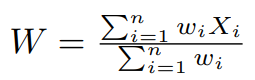
In this calculation, X i  represents the price at which buy orders are placed, and w i  denotes the corresponding weights, determined by the lot size multiplier. Up to this point, the weighted average price level, W, can be calculated as:

W = 1 × ( Initial Price ) + 2 × ( Initial Price − 15  pips ) 3 ​

Here, X 1 is the Initial Price, X 2 is the Initial Price minus 15 pips, w 1 equals 1, and w 2 equals 2.

The point at which the net profit reaches zero is when the price level aligns with this calculated weighted average price level. The demonstration of this concept is as follows:

Note: For simplicity, we are ignoring the spreads for now.

Let's simplify and consider that the initial price is x, where a buy order with a lot size of 0.01 is opened. If the price then decreases by 15 pips, we place a new buy order at  x − 15  and double the lot size to 0.02. The weighted average price level at this point is calculated as ( 1 × x + 2 × ( x − 15 ) ) / 3 , which equals x − 10 . This is 10 pips below the initial price level.

When the price hits x − 15 , the initial buy order of 0.01 incurs a loss of $1.5 (assuming the EURUSD pair, where $1 is equivalent to 10 pips). If the price then rises to the weighted average level of x − 10 , we recoup a $0.5 loss on the initial order. Additionally, we gain on the new buy order of 0.02, as the price has risen by 5 pips from the level of x − 15 . Due to the doubled lot size, our gain here is also doubled, amounting to $1. Thus, our total net profit equals $0 (which is -$1.5 + $0.5 + $1).

If the price increases further from the weighted average level of x − 10 , we continue to earn profits until it reaches the take-profit level.

If the price, instead of rising, continues to fall from the weighted average price level, we apply the same strategy. Should the price drop below x − 15  by another 15 pips, a new buy order is placed at x − 30 , with the lot size again doubling from the previous one, now to 0.04 (2 times 0.02). The new weighted average price level is calculated as ( 1 × x + 2 × ( x − 15 ) + 4 × ( x − 30 ) ) / 7 , which simplifies to x − 21.428 , positioning it 21.428 pips below the initial price level.

At the price level of x − 30 , the initial buy order of 0.01 faces a loss of $3.0 (assuming the EURUSD pair, where $1 is equivalent to 10 pips). The second buy order of 0.02 incurs a loss of 2 times $1.5, equating to $3.0, leading to a total loss of $6.0. However, if the price then ascends to the weighted average level of x − 21.428 , the loss on the initial buy order of 0.01 is partly recouped by $0.8572. Additionally, the loss on the second order of 0.02 is offset by 2 times $0.8572, which is $1.7144. Furthermore, we profit from the new buy order of 0.04 as the price has increased by 8.572 pips from the level of x − 30 . Due to the quadrupled lot size (0.04), our gain is also quadrupled, amounting to 4 times $0.8572, which is $3.4288. Thus, the total net profit will be approximately $0 ( -$6 + $0.8572 + $1.7144 + $3.4288 = $0.0004). This figure is not exactly zero due to rounding off in the weighted average price level calculation.

Should the price further ascend from the weighted average level of x − 21.428 , we will continue to accumulate positive profits until reaching the take-profit level. Conversely, if the price falls again, we repeat the process, doubling the lot size with each iteration and adjusting the weighted average price level accordingly. This approach ensures that we consistently achieve a net profit of approximately $0 each time the price hits the weighted average price level, gradually leading to positive profits.

This same process is applicable for sell orders, starting the cycle with an initial sell order. Let's break it down:

We begin with a sell position at a certain initial price, using a small lot size for simplicity, say 0.01 (the minimum possible size). From here, two outcomes are possible: the price may either rise or fall. If the price falls, we profit based on the extent of the decline and realize this profit when the price reaches our take-profit level. However, the situation becomes challenging when the price starts rising, at which point our classic grid strategy is employed to ensure profits.

Suppose the price increases by a certain amount, for ease of explanation let's say 15 pips. In response, we place another sell order at the initial price plus 15 pips, and we double the lot size for simplicity's sake, making the lot size multiplier 2. After placing this new sell order, two scenarios emerge: the price can either continue to rise or start to fall. If the price falls, we profit from this new sell order due to the increased lot size. Additionally, this decrease not only results in profits but also lessens the loss on our initial sell order of lot size 0.01. We reach a net profit of zero when the price hits the weighted average price level of both orders, a concept we've already explored while discussing buy orders.

The formula for calculating the weighted average remains the same, taking into account the respective prices and lot sizes of the orders. This strategic approach ensures that even in fluctuating markets, our position remains guarded against losses, achieving break-even points or profits as the market moves.

For simplicity, let's assume the initial price is x  where a sell order with a lot size of 0.01 is placed. If the price then rises by 15 pips, we place a new sell order at x + 15 , doubling the lot size to 0.02. The weighted average price level at this stage is calculated as ( 1 × x + 2 × ( x + 15 ) ) / 3 , which simplifies to x + 10 , or 10 pips above the initial price level.

When the price reaches x + 15 , the initial sell order of 0.01 incurs a loss of $1.5 (assuming the EURUSD pair where $1 is equivalent to 10 pips). If the price then drops to the weighted average level of x + 10 , we offset a $0.5 loss on the initial sell order. In addition, we also gain from the new sell order of 0.02, as the price has decreased by 5 pips from the level of x + 15 . Due to the doubled lot size, our gain is also doubled, resulting in $1. Hence, our total net profit equals $0 (calculated as -$1.5 + $0.5 + $1).

Should the price continue to decrease from the weighted average level of x + 10 , we will accrue positive profits until reaching the take-profit level. This strategy effectively balances the losses and gains across different price movements, ensuring a net profit or break-even scenario under varying market conditions.

If the price, contrary to decreasing, continues to rise from the weighted average price level, we apply the same strategy as before. Let's say the price surpasses the x + 15  level by another 15 pips. In response, we place a new sell order at x + 30 , again doubling the lot size from the previous one, now to 0.04 (2 times 0.02). The revised weighted average price level is then calculated as ( 1 × x + 2 × ( x + 15 ) + 4 × ( x + 30 ) ) / 7 , which simplifies to x + 21.428 , or 21.428 pips above the initial price level.

At the price level of x + 30 , the initial sell order of 0.01 faces a loss of $3.0 (assuming the EURUSD pair, where $1 is equivalent to 10 pips). The second sell order of 0.02 incurs a loss of 2 times $1.5, equating to $3.0, leading to a total loss of $6.0. However, if the price then drops to the weighted average level of x + 21.428 , we partially recover the loss on the initial sell order of 0.01 by $0.8572. Additionally, we recoup the loss on the second order of 0.02 by 2 times $0.8572, which is $1.7144. Moreover, we profit from the new sell order of 0.04 as the price has decreased by 8.572 pips from the level of x + 30 . Due to the quadrupled lot size (0.04), our gain is also quadrupled, amounting to 4 times $0.8572, which is $3.4288. Thus, the total net profit will be approximately $0 (calculated as -$6 + $0.8572 + $1.7144 + $3.4288 = $0.0004). This figure is not exactly zero due to rounding off in the weighted average price level calculation.

Should the price continue to drop from the weighted average level of x + 21.428 , we will accumulate positive profits until reaching the take-profit level. Conversely, if the price rises further, we repeat the process, doubling the lot size with each iteration and adjusting the weighted average price level accordingly. This approach ensures that we consistently achieve a net profit of approximately $0 each time the price hits the weighted average price level, gradually leading to positive profits.

Discussing Automation of our Classic Grid Strategy

Now, let's delve into the automation of this classic grid strategy using an Expert Advisor (EA).

First, we will declare a few input variables in the global space:

input bool initialPositionBuy = true;
input double distance = 15;
input double takeProfit = 5;
input double initialLotSize = 0.01;
input double lotSizeMultiplier = 2;

1. initialPositionBuy: A boolean variable determining the type of initial position – either a buy or sell position. If set to true, the initial position will be a Buy; otherwise, it will be a Sell.
2. distance: The fixed distance, measured in pips, between each consecutive order.
3. takeProfit: The distance, measured in pips, above the average price of all open positions at which all positions will be closed for a total net profit.
4. initialLotSize: The lot size of the first position.
5. lotSizeMultiplier: The multiplier applied to the lot size for each consecutive position.

These are the input variables which we will be changing for various purposes such as optimization in our strategy. Now we will define some more variables in the global space:

bool gridCycleRunning = false;
double lastPositionLotSize, lastPositionPrice, priceLevelsSumation, totalLotSizeSummation;

These variables will be used for the following purposes:

1. gridCycleRunning: This is a boolean variable which will be true if cycle is running and false otherwise and by default it is false.
2. lastPositionLotSize: This is a double variable created to store the lot size of the last opened position at any given point of time in the cycle.
3. lastPositionPrice: This is a double variable created to store the open price level of the last position at any given point of time in the cycle.
4. priceLevelsSumation: This is the summation over all the open price level of all positions which will later be used in calculating the average price level.
5. totalLotSizeSummation: This is the summation over all the lot sizes of all the positions which will later be used in calculating the average price level.

Now that we have established the key input variables, we will proceed with an essential function, StartGridCycle(), which will handle the initialization of the cycle.

//+------------------------------------------------------------------+
//| Hedge Cycle Intialization Function                               |
//+------------------------------------------------------------------+
void StartGridCycle()
   {
    double initialPrice = initialPositionBuy ? SymbolInfoDouble(_Symbol, SYMBOL_ASK) : SymbolInfoDouble(_Symbol, SYMBOL_BID);

    ENUM_ORDER_TYPE positionType = initialPositionBuy ? ORDER_TYPE_BUY : ORDER_TYPE_SELL;
    m_trade.PositionOpen(_Symbol, positionType, initialLotSize, initialPrice, 0, 0);

    lastPositionLotSize = initialLotSize;
    lastPositionPrice = initialPrice;
    ObjectCreate(0, "Next Position Price", OBJ_HLINE, 0, 0, lastPositionPrice - distance * _Point * 10);
    ObjectSetInteger(0, "Next Position Price", OBJPROP_COLOR, clrRed);

    priceLevelsSumation = initialLotSize * lastPositionPrice;
    totalLotSizeSummation = initialLotSize;

    if(m_trade.ResultRetcode() == 10009)
        gridCycleRunning = true;
   }
//+------------------------------------------------------------------+

In the StartGridCycle() function, we first create a double variable, initialPrice , which will store either the ask or bid price, contingent on the initialPositionBuy variable. Specifically, if initialPositionBuy is true, we store the ask price; if it is false, we store the bid price. This distinction is crucial because a buy position can only be opened at the ask price, while a sell position must be opened at the bid price.

ENUM_ORDER_TYPE positionType = initialPositionBuy ? ORDER_TYPE_BUY : ORDER_TYPE_SELL;
CTrade m_trade;
m_trade.PositionOpen(_Symbol, positionType, initialLotSize, initialPrice, 0, 0);

Now, we will open either a buy or sell position based on the value of initialPositionBuy . To achieve this, we will create a variable named positionType of the ENUM_ORDER_TYPE type. ENUM_ORDER_TYPE is a predefined custom variable type in MQL5, capable of taking integer values from 0 to 8, each representing a specific order type as defined in the following table:

Integer Values	Identifier
0	ORDER_TYPE_BUY
1	ORDER_TYPE_SELL
2	ORDER_TYPE_BUY_LIMIT
3	ORDER_TYPE_SELL_LIMIT
4	ORDER_TYPE_BUY_STOP
5	ORDER_TYPE_SELL_STOP
6	ORDER_TYPE_BUY_STOP_LIMIT
7	ORDER_TYPE_SELL_STOP_LIMIT
8	ORDER_TYPE_CLOSE_BY

Indeed, within the ENUM_ORDER_TYPE , the values 0 and 1 correspond to ORDER_TYPE_BUY and ORDER_TYPE_SELL , respectively. For our purposes, we will focus on these two. Utilizing the identifiers rather than their integer values is advantageous, as identifiers are more intuitive and easier to remember.

Therefore, we set positionType to ORDER_TYPE_BUY if initialPositionBuy is true; otherwise, we set it to ORDER_TYPE_SELL .

To proceed, we first import the standard trade library Trade.mqh in the global space. This is done using the following statement:

#include <Trade/Trade.mqh>
CTrade m_trade;

To continue, we also define an instance of the CTrade class, which we'll name m_trade . This instance will be used to manage trade operations. Then, to open a position, we utilize the PositionOpen function from m_trade , which handles the actual opening of buy or sell positions based on the parameters we've set, including the positionType and other relevant trade settings.

m_trade.PositionOpen(_Symbol, positionType, initialLotSize, initialPrice, 0, 0);

In using the PositionOpen function from the m_trade instance, we provide it with several parameters essential for opening a position:

1. _Symbol: The first parameter is _Symbol , which refers to the current trading symbol.

2. positionType: The second parameter is positionType , which we defined earlier based on the value of initialPositionBuy . This determines whether the position opened is a buy or sell.

3. initialLotSize: The lot size for the position, as defined by our input variable initialLotSize .

4. initialPrice: The price at which the position is opened. This is determined by the initialPrice variable, which holds either the ask or bid price depending on the type of position to be opened.
   

5. SL (Stop Loss) and TP (Take Profit): The last two parameters are for setting Stop Loss (SL) and Take Profit (TP). In this specific strategy, we do not set these parameters initially, as the closing of orders will be determined by the strategy logic, particularly when the price reaches the average price plus the takeProfit value.

Now, let's move to the next part of the code:

lastPositionLotSize = initialLotSize;
lastPositionPrice = initialPrice;
ObjectCreate(0, "Next Position Price", OBJ_HLINE, 0, 0, lastPositionPrice - distance * _Point * 10);
ObjectSetInteger(0, "Next Position Price", OBJPROP_COLOR, clrRed);

1. Setting the lastPositionLotSize and lastPositionPrice Variables:

   • We've initialized the lastPositionLotSize variable, defined in the global space, to equal initialLotSize . This variable is crucial as it keeps track of the lot size of the most recently opened position, enabling the calculation of the lot size for the next order by multiplying it with the input multiplier.
   • Similarly, lastPositionPrice is also set to initialPrice. This variable, also defined in the global space, is essential for determining the price level at which subsequent orders should be opened.
     
     

2. Creating a Horizontal Line for Visualization:

   • To enhance the visual representation of our strategy on the chart, we use the ObjectCreate function. This function is given the following parameters:
     • 0 for the current chart
     • "Next Position Price" as the name of the object
     • OBJ_HLINE as the object type, indicating a horizontal line
     • Two additional 0 s, one for the sub-window and the other for datetime, since only the price level is needed for a horizontal line
     • The calculated price level for the next order, (lastPositionPrice - distance * _Point * 10) , as the final parameter
   • To set the color of this horizontal line to red, we use the ObjectSetInteger function with the OBJPROP_COLOR property set to clrRed.
     
     

3. Proceeding with Average Price Management in a Grid Cycle:

   • With these initial steps completed, we now move on to manage the average price within the grid cycle. This involves dynamically calculating and adjusting the average price as new positions are opened and the market evolves, a key component in the grid trading strategy.

Let's move forward with the next part of your code implementation.

priceLevelsSumation = initialLotSize * lastPositionPrice;
totalLotSizeSummation = initialLotSize;

1. Setting priceLevelsSumation :

   • We've defined priceLevelsSumation in the global space to calculate the weighted average price of all open positions. Initially, since there's only one order, we set priceLevelsSumation equal to the lastPositionPrice multiplied by its corresponding weight, which is the lot size of the order. This setup prepares the variable to accumulate more price levels, each multiplied by their respective lot sizes, as new positions are opened.

2. Initializing totalLotSizeSummation :

   • The totalLotSizeSummation variable is initially set equal to initialLotSize. This makes sense in the context of the weighted average formula, where we need to divide by the total weights. At the beginning, with just one order, the total weight is the lot size of that single order. As you open more positions, we will add their weights (lot sizes) to this summation, thus dynamically updating the total weight.

Now, let's proceed with the last part of the StartGridCycle() function:

if(m_trade.ResultRetcode() == 10009)
    gridCycleRunning = true;

Setting hedgeCycleRunning :

• The variable hedgeCycleRunning is set to true only after a position is successfully opened. This is verified using the ResultRetcode() function from the CTrade instance, named trade . The return code "10009" indicates successful placement of the order. (Note: The various return codes can be referenced for different outcomes of trade requests.)
• The use of hedgeCycleRunning is pivotal for the strategy, as it flags the commencement of the grid cycle. The significance of this flag will become more apparent in subsequent parts of the code.

Having completed the StartGridCycle() function, which initiates the grid strategy, you now move to the OnTick() function. We divide this function in 5 segments, each handling a specific aspect of the trading logic:

1. Starting Grid Cycle
2. Handling Buy Positions
3. Handling Sell Positions
4. Grid Cycle Closing Function
5. Handling Positions Closing

1. Starting Grid Cycle:
   

   double price = initialPositionBuy ? SymbolInfoDouble(_Symbol, SYMBOL_ASK) : SymbolInfoDouble(_Symbol, SYMBOL_BID);
     
     if(!gridCycleRunning)
        {
         StartGridCycle();
        }

   1. Declaring the price Variable:

      • A new variable, named price, is declared. Its value is determined by the initialPositionBuy flag:
        • If initialPositionBuy is true, price is set to the current ASK price.
        • If initialPositionBuy is false, price is set to the current BID price.

   2. Conditional Execution Based on gridCycleRunning:

      • The next step involves a conditional check on the gridCycleRunning variable:
        • If gridCycleRunning is false, this indicates that the grid cycle hasn't started yet or has completed its previous cycle. In this case, we execute the StartGridCycle() function, which was thoroughly explained earlier. This function initializes the grid cycle by opening the first position and setting up the necessary parameters.
        • If gridCycleRunning is true, it implies that the grid cycle is already active. In this scenario, we choose to do nothing for the moment. This decision allows the existing grid cycle to continue operating based on its established logic without initiating a new cycle or interfering with the current one.

   This approach efficiently manages the initiation and continuation of the grid cycle, ensuring that the trading strategy adheres to its designed operational flow. Let's proceed with the next steps in the grid strategy implementation.

   
   

2. Handling Buy Positions:
   

   if(initialPositionBuy && price <= lastPositionPrice - distance * _Point * 10 && gridCycleRunning)
        {
         double newPositionLotSize = NormalizeDouble(lastPositionLotSize * lotSizeMultiplier, 2);
         m_trade.PositionOpen(_Symbol, ORDER_TYPE_BUY, newPositionLotSize, price, 0, 0);
     
         lastPositionLotSize *= lotSizeMultiplier;
         lastPositionPrice = price;
         ObjectCreate(0, "Next Position Price", OBJ_HLINE, 0, 0, lastPositionPrice - distance * _Point * 10);
         ObjectSetInteger(0, "Next Position Price", OBJPROP_COLOR, clrRed);
     
         priceLevelsSumation += newPositionLotSize * lastPositionPrice;
         totalLotSizeSummation += newPositionLotSize;
         ObjectCreate(0, "Average Price", OBJ_HLINE, 0, 0, priceLevelsSumation / totalLotSizeSummation);
         ObjectSetInteger(0, "Average Price", OBJPROP_COLOR, clrGreen);
        }

   Here, We have another if-statement that has 3 conditions:

   1. Condition on initialPositionBuy :

      • The segment of code is executed only if the variable initialPositionBuy is true. This condition ensures that the logic for handling buy positions is separated from that of sell positions.
        
        

   2. Condition on price :

      • The second condition checks whether the variable price is less than or equal to lastPositionPrice - distance * _Point * 10 . This condition is crucial for determining when to open a new buy position. The subtraction (-) operation is used here, aligning with the directional logic defined in your grid strategy for buy positions.
        
        

   3. Condition on gridCycleRunning :

      • The third condition requires that the variable gridCycleRunning be true, indicating that the grid cycle is currently active. This is essential to ensure that new positions are only opened as part of an ongoing trading cycle.
        
        

   If all three conditions are met, the EA proceeds to open a new buy position. However, before doing so, it calculates the lot size for the new position:

   • A new double variable, newPositionLotSize , is declared and set equal to lastPositionLotSize multiplied by lotSizeMultiplier .
   • The resulting lot size is then normalized to two decimal places to make the lot size valid since lot size has to be strict multiple of 0.01.
     
     

   This approach ensures that new positions are opened at appropriate sizes, adhering to the grid strategy's rules. Subsequently, the EA utilizes the PositionOpen() function from the CTrade class instance named m_trade (declared earlier in the global space) to open the buy position with the calculated lot size.

   Continuing with the logic, the next step involves updating the lastPositionLotSize variable. This is crucial for maintaining the accuracy of lot sizes in subsequent orders:

   • The lastPositionLotSize is set equal to itself multiplied by lotSizeMultiplier. Crucially, this multiplication does not involve normalization to two decimal places.
   • The reason for avoiding normalization is illustrated by considering a scenario where the lotSizeMultiplier is 1.5 and the initialLotSize is 0.01. Multiplying 0.01 by 1.5 results in 0.015, which, when normalized to two decimal places, rounds back to 0.01. This creates a loop where the lot size remains constantly at 0.01, despite being multiplied.
   • To avoid this issue and ensure the lot sizes increase as intended, lastPositionLotSize is updated using the unnormalized product of itself and the lotSizeMultiplier. This step is critical for the grid strategy to function correctly, especially with fractional multipliers.
     
     

   With this update, the EA accurately tracks and adjusts the lot sizes for new positions, maintaining the intended progression of the grid strategy.

   Continuing with the process, the next step involves updating the lastPositionPrice and visualizing the next position level on the chart:

   1. Updating lastPositionPrice :
      • The variable lastPositionPrice is updated equal to price, which is determined by the initialPositionBuy condition. Since the first condition of the if-statement ensures entry only when initialPositionBuy is true, price will correspond to the ASK price in this context.
        
        
   2. Visualizing the Next Position Level:
      • A horizontal line, named "Next Position Price", is drawn on the chart. This line represents the price level at which the next order will be opened.
      • Since initialPositionBuy is true, indicating that the next position will be a buy, the price level for this line is set to lastPositionPrice (which was just updated) minus the distance (as specified in the inputs) multiplied by _Point and then further multiplied by 10.
      • This horizontal line is created using the ObjectCreate() function, and its color is set to clrRed using additional object properties functions for easy visualization. This visual aid helps in easily identifying the price level for the next potential buy order.
        
        

   By updating lastPositionPrice and visually marking the next order level, the EA effectively prepares for the subsequent steps in the grid cycle, ensuring that each new position aligns with the strategy's criteria and is visually trackable on the chart.

   Now, let's refine the calculation of the average price level, specifically focusing on the weighted average:

   1. Updating priceLevelsSummation and totalLotSizeSummation :

      • To update the weighted average price, we add the product of lastPositionPrice and newPositionLotSize to priceLevelsSummation.
      • For totalLotSizeSummation, we simply add the value of newPositionLotSize.
      • These updates are crucial for keeping track of the cumulative price levels and total lot sizes of all positions.
        
        

   2. Calculating the Weighted Average Price Level:

      • The average price level, which is a weighted average in this context, is calculated by dividing priceLevelsSummation by totalLotSizeSummation.
      • This calculation accurately reflects the average price of all open positions, taking into account their respective lot sizes.
        
        

   3. Visualizing the Weighted Average Price Level:

      • Another horizontal line is created on the chart at the calculated average price level using the ObjectCreate() function.
      • The color of this line is set to clrGreen, differentiating it from the other horizontal line indicating the next position price.
      • It's important to note that the normalized value of lastPositionLotSize multiplied by lotSizeMultiplier is used for this calculation. This ensures that the real lot size of the newly opened position is considered, providing an accurate weighted average.
        
        

   By incorporating these steps, the EA not only keeps track of the average price level of all open positions but also visually represents it on the chart. This allows for easy monitoring and decision-making based on the current state of the grid cycle and market conditions.

   
   

3. Handling Sell Positions:
   

   if(!initialPositionBuy && price >= lastPositionPrice + distance * _Point * 10 && gridCycleRunning)
        {
         double newPositionLotSize = NormalizeDouble(lastPositionLotSize * lotSizeMultiplier, 2);
         m_trade.PositionOpen(_Symbol, ORDER_TYPE_SELL, newPositionLotSize, price, 0, 0);
     
         lastPositionLotSize *= lotSizeMultiplier;
         lastPositionPrice = price;
         ObjectCreate(0, "Next Position Price", OBJ_HLINE, 0, 0, lastPositionPrice + distance * _Point * 10);
         ObjectSetInteger(0, "Next Position Price", OBJPROP_COLOR, clrRed);
     
         priceLevelsSumation += newPositionLotSize * lastPositionPrice;
         totalLotSizeSummation += newPositionLotSize;
         ObjectCreate(0, "Average Price", OBJ_HLINE, 0, 0, priceLevelsSumation / totalLotSizeSummation);
         ObjectSetInteger(0, "Average Price", OBJPROP_COLOR, clrGreen);
        }

   Here, We have another if-statement that has again 3 conditions:

   1. Condition on initialPositionBuy :

      • This segment of the code is executed only if initialPositionBuy is false. This condition ensures that the logic specifically handles sell positions, distinct from buy positions.
        
        

   2. Condition on price :

      • The second condition checks whether price is greater than or equal to lastPositionPrice + distance * _Point * 10 . This is essential for determining the right moment to open a new sell position. The addition (+) operation is used in this case, aligning with the directional logic of your strategy for sell positions.
        
        

   3. Condition on gridCycleRunning :

      • The third condition requires that gridCycleRunning be true, indicating that the grid cycle is actively running. This ensures that new positions are only opened as part of the ongoing trading cycle.
        
        

   If all three conditions are met, the EA proceeds to open a new sell position:

   • A double variable newPositionLotSize is declared and set equal to lastPositionLotSize multiplied by lotSizeMultiplier.
   • This new lot size is then normalized to two decimal places to make the lot size valid since lot size has to be strict multiple of 0.01.
   • Finally, the EA uses the PositionOpen() function from the CTrade class instance m_trade (declared earlier in the global space) to open the sell position with the calculated lot size.
     
     

   This approach ensures that new sell positions are opened at appropriate intervals and sizes, adhering to the grid strategy's rules and maintaining the strategy's progression.

   In the next step of handling sell positions, we focus on correctly updating the lastPositionLotSize variable:

   • The variable lastPositionLotSize is updated to be equal to itself multiplied by the lotSizeMultiplier. This step is crucial for maintaining the progression of lot sizes in the grid cycle.
   • Importantly, this multiplication does not involve normalization to two decimal places. This decision is critical to avoid a potential issue with fractional multipliers.
   • To illustrate: with a lotSizeMultiplier of 1.5 and an initialLotSize of 0.01, the multiplication would result in 0.015. Normalizing this to two decimal places would round it back to 0.01. Repeating this process would perpetually yield a lot size of 0.01, creating a loop and undermining the strategy's intention.
   • To circumvent this problem, lastPositionLotSize is set to the unnormalized product of itself and the lotSizeMultiplier. This approach ensures that the lot sizes increase appropriately, especially when dealing with multipliers that result in fractional lot sizes.
     
     

   By updating the lastPositionLotSize without normalization, the EA effectively tracks and adjusts the lot sizes for new sell positions, ensuring that the grid strategy functions as intended.

   1. Updating lastPositionPrice :

      • The variable lastPositionPrice is updated to equal price, which will be either the ASK or BID price depending on the value of initialPositionBuy .
      • In this case, since we enter this segment of the code only if initialPositionBuy is false (as per the first condition), lastPositionPrice is set to the BID price.
        
        

   2. Drawing a Horizontal Line for the Next Position:

      • A horizontal line named "Next Position Price" is drawn on the chart. This line indicates the price level where the next order (a sell order, in this case) will be opened.
      • The price level for this horizontal line is set to lastPositionPrice (which has been updated) plus the distance specified in the inputs, multiplied by _Point and then further multiplied by 10. This calculation determines the appropriate level for the next sell order.
      • The line is created using the ObjectCreate() function, a predefined function in MQL5 for drawing objects on charts.
      • The color of this line is set to clrRed, enhancing its visibility and making it easy to distinguish on the chart.
        
        

   By setting lastPositionPrice appropriately and visually representing the next order's level, the EA effectively prepares for subsequent sell orders, ensuring they align with the grid strategy’s rules and are easily identifiable on the chart.

   In handling the calculation of the average price level, specifically focusing on the weighted average for sell positions, the process involves:

   1. Updating priceLevelsSummation and totalLotSizeSummation :

      • The value of lastPositionPrice multiplied by newPositionLotSize is added to priceLevelsSummation. This step accumulates the price levels of all open positions, each weighted by their respective lot sizes.
      • The value of newPositionLotSize is added to totalLotSizeSummation. This variable keeps track of the cumulative lot sizes of all positions.
        
        

   2. Calculating the Weighted Average Price Level:

      • The average price level is obtained by dividing priceLevelsSummation by totalLotSizeSummation. This calculation yields the weighted average price of all open positions.
        
        

   3. Visualizing the Weighted Average Price Level:

      • A horizontal line is created at the weighted average price level using the ObjectCreate() function. This visual representation helps in monitoring the average price of all positions.
      • The color of this line is set to clrGreen, making it easily distinguishable from other lines on the chart.
      • It’s important to note that the normalized value of lastPositionLotSize multiplied by lotSizeMultiplier is used in these calculations. This ensures that the actual, real lot sizes of the opened positions are considered, providing an accurate weighted average calculation.
        
        

   This method of calculating and visualizing the weighted average price level is crucial for the effective management of sell positions in the grid cycle, allowing for informed decision-making based on the current market and position status.

   
   

4. Grid Cycle Closing Function:
   

   //+------------------------------------------------------------------+
   //| Stop Function for a particular Grid Cycle                        |
   //+------------------------------------------------------------------+
   void StopGridCycle()
      {
       gridCycleRunning = false;
       ObjectDelete(0, "Next Position Price");
       ObjectDelete(0, "Average Price");
       for(int i = PositionsTotal() - 1; i >= 0; i--)
          {
           ulong ticket = PositionGetTicket(i);
           if(PositionSelectByTicket(ticket))
              {
               m_trade.PositionClose(ticket);
              }
          }
      }
   //+------------------------------------------------------------------+

   1. Setting gridCycleRunning to False:

      • The first action in this function is to set the boolean variable gridCycleRunning to false. This change signifies that the grid cycle is no longer active and is in the process of closing.
        
        

   2. Deleting Chart Objects:

      • Next, you use the predefined ObjectDelete() function to remove two specific objects from the chart: "Next Position Price" and "Average Price". This step clears the chart of these markers, indicating that the cycle is concluding and these price levels are no longer relevant.
        
        

   3. Closing All Positions:

      • The function then proceeds to loop through all open positions.
      • Each position is selected individually by its ticket number.
      • Once a position is selected, it is closed using the PositionClose() function from the m_trade instance. The ticket number of the position is passed as a parameter to this function.
      • This systematic approach ensures that all positions opened as part of the grid cycle are closed, effectively winding up the trading activity for that particular cycle.
        
        

   By following these steps, the Grid Cycle Closing Function methodically and efficiently closes all open positions, resets the trading environment, and prepares the EA for a new grid cycle.

   
   

5. Handling Positions Closing:
   

   if(gridCycleRunning)
      {
       if(initialPositionBuy && price >= (priceLevelsSumation / totalLotSizeSummation) + takeProfit * _Point * 10)
           StopGridCycle();
   
       if(!initialPositionBuy && price <= (priceLevelsSumation / totalLotSizeSummation) - takeProfit * _Point * 10)
           StopGridCycle();
      }

   In the final section, "Handling Positions Closing," the process for closing orders is controlled by an if-statement, contingent on certain conditions:

   1. The primary condition for any action to take place is that gridCycleRunning must be true, indicating an active grid cycle.
   2. Within this, there are two further conditional checks based on the value of initialPositionBuy:
      • If initialPositionBuy is true and the current price is takeProfit pips (defined in the input variables) above the weighted average price level, then the StopGridCycle() function is executed.
      • Conversely, if initialPositionBuy is false and the current price is takeProfit pips below the weighted average price level, the StopGridCycle() function is executed.
        
        

   These conditions ensure that the grid cycle stops and positions are closed based on the specified take-profit criteria relative to the weighted average price level.This marks the conclusion of the automation process for the Classic Grid Strategy.

   
   

Backtesting the Classic Grid Strategy

With the automation of our Classic Grid Strategy now complete, it's time to evaluate its performance in a real-world scenario.

For the backtest, the following input parameters will be used:

• initialPositionBuy : true
• distance : 15 pips
• takeProfit : 5 pips
• initialLotSize : 0.01
• lotSizeMultiplier : 2.0

The testing will be conducted on the EURUSD pair, spanning from November 1, 2023, to December 22, 2023. The chosen leverage is 1:500, with a starting deposit of $10,000. As for the timeframe, it's noteworthy that it's irrelevant to our strategy, so any selection will suffice without impacting the results. This test, although covering a relatively short period of just under two months, aims to serve as a representative sample for potential outcomes over longer durations.

Now, let's delve into the results of this backtest:

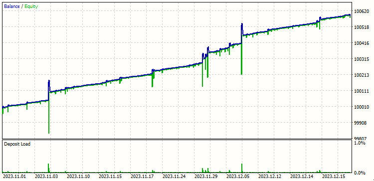
These results look quite good. Upon reviewing the backtest results, we observe intriguing trends represented by the blue and green lines in the graph. Let’s break down what each line signifies and how their movements reflect the strategy's performance:

1. Understanding the Blue and Green Lines:

   • The blue line represents the account balance, while the green line indicates the equity.
   • A notable pattern is observed where the balance increases, the equity decreases, and eventually, they converge at the same point.
     
     

2. Explanation for Balance Fluctuations:

   • The strategy dictates closing all orders of a cycle simultaneously, which should ideally result in a straightforward increase in balance. However, the graph shows a pattern of rise and fall in the balance, which requires further explanation.
   • This fluctuation is attributed to the slight delay (fractions of a second) in closing orders. Even though the orders are closed almost simultaneously, the graph captures the incremental updates in balance.
   • Initially, the balance increases as profitable positions close first. The positions are closed in a loop, starting from the last (most profitable) position, as indicated by the function PositionsTotal(). Therefore, the upward and brief downward movement in the balance line can be disregarded, focusing instead on the net upward trend.
     
     

3. Equity Line Movement:

   • Corresponding to the balance, the equity initially dips and then rises. This is because the profitable positions are closed first, temporarily reducing the equity before it recovers.
   • The movement of the green equity line follows a similar logic to the blue balance line, leading to the same conclusion of an overall positive trend.

In summary, despite the minor fluctuations captured in the graph due to the order-closing sequence and slight delays, the overarching trend indicates a successful outcome of the strategy, as evidenced by the final convergence and upward movement of both the balance and equity lines.

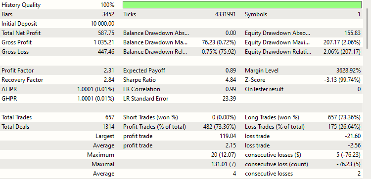
The backtest results demonstrate profitability for the Classic Grid Strategy. However, it's important to recognize a significant limitation inherent in this strategy: the requirement for high holding capacity.

This strategy often necessitates substantial capital to withstand the drawdowns that occur before reaching profitability. The ability to hold positions through adverse market movements without facing margin calls or being forced to close positions at a loss is crucial.

Addressing this limitation will be a key focus in the subsequent parts of our series, where we'll explore optimization techniques for this strategies. The aim will be to enhance their efficiency and reduce the required holding capacity, making the strategy more accessible and less risky for traders with varying capital sizes.

Conclusion

In this installment, we delved into the intricacies of the classic grid strategy, successfully automating it using an Expert Advisor (EA) in MQL5. We also examined some initial results of this strategy, highlighting its potential and areas for improvement.

However, our journey towards optimizing such strategies is far from over. Future parts of this series will focus on fine-tuning the strategy, particularly honing in on the optimal values for input parameters like distance, takeProfit, initialLotSize, and lotSizeMultiplier to maximize returns and minimizing drawdowns. An intriguing aspect of our upcoming exploration will be determining the efficacy of starting with a buy or sell position, which may vary depending on different currencies and market conditions.

There's much to look forward to in our subsequent articles, where we'll uncover more valuable insights and techniques. I appreciate your time in reading my articles and hope they offer both knowledge and practical aid in your trading and coding pursuits. If there are specific topics or ideas you'd like to see discussed in the next part of this series, your suggestions are always welcome.

Happy Coding! Happy Trading!