Neural networks made easy (Part 56): Using nuclear norm to drive research

Introduction
Reinforcement learning is based on the paradigm of independent exploration of the environment by the Agent. The Agent affects the environment, which leads to its change. In return, the Agent receives some kind of reward.
This is where the two main problems of the reinforcement learning are highlighted: environment exploration and the reward function. A correctly structured reward function encourages the Agent to explore the environment and search for the most optimal behavioral strategies.
However, when solving most practical problems, we are faced with sparse external rewards. To overcome this barrier, the use of so-called internal rewards was proposed. They allow the Agent to master new skills that may be useful for obtaining external rewards in the future. However, internal rewards may be noisy due to environmental stochasticity. Directly applying noisy forecast values to observations can negatively impact the efficiency of Agent policy training. Moreover, many methods use L2 norm or variance to measure the novelty of a study, which increases noise due to the squaring operation.
To solve this problem, the article "Nuclear Norm Maximization Based Curiosity-Driven Learning" proposes a new algorithm for stimulating the Agent's curiosity based on nuclear norm maximization (NNM). Such an internal reward is able to evaluate the novelty of environmental exploration more accurately. At the same time, it allows for high immunity to noise and spikes.
1. Nuclear norm and its application
Matrix norms, including the nuclear norm, are widely used in the analysis and computational methods of linear algebra. The nuclear norm plays an important role in the study of properties of matrices, optimization problems, conditionality assessment and many other areas of mathematics and applied sciences.
The nuclear norm of a matrix is a numerical characteristic that determines the "size" of the matrix. It is a special case of the Schatten norm and is equal to the sum of the matrix singular values.
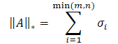
where σi represents the elements of the singular value vector of the A matrix.
At its core, the nuclear norm is the convex hull of the rank function for a set of matrices with the same spectral norm. This allows it to be used in solving various optimization problems.
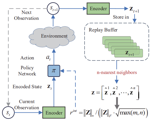
The main idea of the Nuclear Norm Maximization (NNM) method is to accurately estimate novelty using the nuclear norm of a matrix upon visiting a state, while mitigating the effects of noise and various spikes. The matrix of n*m size comprises n coded states of the environment. Each state has the m dimension. The matrix combines the current state of s and its (n - 1) nearest adjacent states. Here s represents an abstract state by mapping the original high-dimensional observation into a low-dimensional abstract space. Since each row of the S matrix represents the encoded state,rank(S) can be used to represent diversity within a matrix. Higher S matrix rank means a larger linear distance between encoded states. The method authors take a creative approach to solving the problem and use matrix rank maximization to increase the research diversity. This encourages our model's Agent to visit more different states with high diversity.
There are two approaches to using the maximum rank of a matrix. We can use it as a loss function or as a reward. Maximizing the matrix rank directly is a rather difficult problem with a non-convex function. Therefore, we will not use it as a loss function. However, the rank value of the matrix is discrete and cannot accurately reflect the novelty of states. Therefore, using the raw matrix rank value as a reward to guide model training is also inefficient.
Mathematically, the calculation of a matrix rank is usually replaced by its nuclear norm. Therefore, novelty can be maintained by approximate maximization of the nuclear norm. Compared to rank, nuclear norm has several good properties. First, the convexity of the nuclear norm allows the development of fast and convergent optimization algorithms. Secondly, the nuclear norm is a continuous function, which is important for many training tasks.
The authors of the NNM method propose to determine internal reward using the equation
![]()
where:
λ is a weight for setting the range of nuclear norm values;
‖S‖⋆ is a nuclear norm of the state matrix;
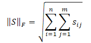
‖S‖F is a Frobenius norm of the state matrix.
We have already become familiar with the nuclear norm of a matrix, while the Frobenius norm is calculated as the square root of the sum of the squares of all matrix elements.
The Cauchy-Bunyakovsky inequality allows us to make the following transformations.
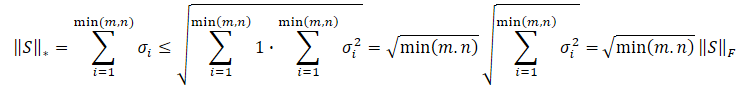
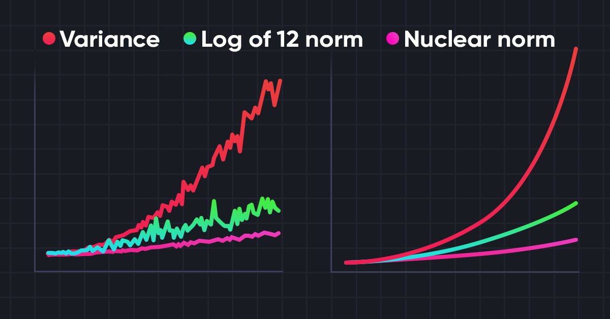
Obviously, the square root of the sum of the value squares will always be less than or equal to the sum of the values themselves. Therefore, the nuclear norm of the matrix will always be greater than or equal to the Frobenius norm of the same matrix. Thus, we can derive the following inequalities.
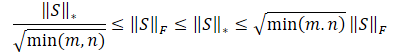
This inequality shows that the nuclear norm and the Frobenius norm constrain each other. If the nuclear norm increases, then the Frobenius norm tends to increase as well.
In addition, the Frobenius norm has another property that is useful for us - it is strictly opposite to entropy in monotonicity. Its increase is equivalent to a decrease in entropy. As a result, the impacts of the nuclear norm can be divided into two parts:
- High variety.
- Low entropy.
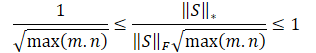
We need to encourage the Agent to visit newer states, and our goal is diversity. However, a decrease in entropy means an increase in the aggregation of states. That means a great similarity of states. Therefore, we aim to encourage the first effect and reduce the influence of the second. To do this, we divide the nuclear norm of a matrix by its Frobenius norm.
Dividing the above inequalities by the Frobenius norm we get the following:
![]()
Obviously, directly using such a reward scale can be detrimental to the model training. In addition, the root of the minimum dimension of the state matrix may vary in different environments or with different architectures of trained models. Therefore, it is desirable to re-normalize our reward scale. Since min(m, n) ≤ max(m, n), we get:
![]()
The above mathematical calculations allow us to automatically determine the adjustment factor for the range of values of the nuclear norm of the λ matrix as
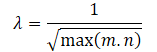
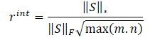
Thus, the internal reward equation will take the form:
Below is the author's visualization of the Nuclear Norm Maximization method.
The test results presented in the author's article demonstrate the superiority of the proposed method over other environmental research algorithms, including the previously reviewed Intrinsic Curiosity Module and Self-Supervised Exploration via Disagreement. In addition, it is noteworthy that the method demonstrates better results when noise is added to the original data. Let's move on to the practical part of our article and evaluate the capabilities of the method in solving our problems.
2. Implementation using MQL5
Before we start implementing the Nuclear Norm Maximization (NNM) method, let's highlight its main innovation - the new internal reward equation. Therefore, this approach can be implemented as a complement to almost any previously considered reinforcement learning algorithm.
It should also be noted that the algorithm uses an encoder to translate environmental states into some kind of compressed representation. The algorithm of k-nearest neighbors is also applied to form a matrix of compressed representations of the environment state.
In my opinion, the simplest solution seems to be the introduction of the proposed internal reward into the RE3 algorithm. It also uses an encoder to translate environmental states into a compressed representation. We use a random convolutional Encoder in RE3 for these purposes. This allows us to reduce the cost of training the encoder.
In addition, RE3 also applies k-nearest environmental conditions for the formation of an internal reward. However, this reward is formed differently.
The direction of our actions is clear, so it is time to get to work. First, we copy all files from the "...\Experts\RE3\" to "...\Experts\NNM\" directory. As you might remember, it contains four files:
- Trajectory.mqh — the library of common constants, structures and methods.
- Research.mq5 — the EA for interacting with the environment and collecting a training sample.
- Study.mq5 — the EA for direct model training.
- Test.mq5 — the EA for testing trained models.
We will also use decomposed rewards. The structure of the reward vector will look as follows.
//+------------------------------------------------------------------+
//| Rewards structure                                                |
//|   0     -  Delta Balance                                         |
//|   1     -  Delta Equity ( "-" Drawdown / "+" Profit)             |
//|   2     -  Penalty for no open positions                         |
//|   3     -  NNM                                                   |
//+------------------------------------------------------------------+
In the "...\NNM\Trajectory.mqh" file, we increase the size of the compressed representation of the environment state and the internal fully connected layer of our models.
#define                    EmbeddingSize   16
#define                    LatentCount    512
The file also contains the CreateDescriptions method for describing the architecture of the models used. Here we will use three neural network models: Actor, Critic and Encoder. We will use a random convolutional Encoder as the latter.
bool CreateDescriptions(CArrayObj *actor, CArrayObj *critic, CArrayObj *convolution)
  {
//---
   CLayerDescription *descr;
//---
   if(!actor)
     {
      actor = new CArrayObj();
      if(!actor)
         return false;
     }
   if(!critic)
     {
      critic = new CArrayObj();
      if(!critic)
         return false;
     }
   if(!convolution)
     {
      convolution = new CArrayObj();
      if(!convolution)
         return false;
     }
In the body of the method, we create a local variable storing a pointer to an object describing one CLayerDescription neural layer and, if necessary, initialize dynamic arrays describing the architectural solutions of the models used.
First, we will create a description of the Actor architecture, which consists of two blocks: source data preliminary processing and decision making.
We submit historical data on the price movement of the analyzed instrument and indicator readings to the input of the initial data preliminary processing block. As you can see, different indicators have different ranges of their parameters. This has a negative impact on the model training efficiency. Therefore, we normalize the received data using the CNeuronBatchNormOCL batch normalization layer.
//--- Actor
   actor.Clear();
//--- Input layer
   if(!(descr = new CLayerDescription()))
      return false;
   descr.type = defNeuronBaseOCL;
   int prev_count = descr.count = (HistoryBars * BarDescr);
   descr.activation = None;
   descr.optimization = ADAM;
   if(!actor.Add(descr))
     {
      delete descr;
      return false;
     }
//--- layer 1
   if(!(descr = new CLayerDescription()))
      return false;
   descr.type = defNeuronBatchNormOCL;
   descr.count = prev_count;
   descr.batch = 1000;
   descr.activation = None;
   descr.optimization = ADAM;
   if(!actor.Add(descr))
     {
      delete descr;
      return false;
     }
We pass the normalized data through two convolutional layers to search for individual indicator patterns.
//--- layer 2
   if(!(descr = new CLayerDescription()))
      return false;
   descr.type = defNeuronConvOCL;
   prev_count = descr.count = BarDescr;
   descr.window = HistoryBars;
   descr.step = HistoryBars;
   int prev_wout=descr.window_out = HistoryBars/2;
   descr.activation = LReLU;
   descr.optimization = ADAM;
   if(!actor.Add(descr))
     {
      delete descr;
      return false;
     }
//--- layer 3
   if(!(descr = new CLayerDescription()))
      return false;
   descr.type = defNeuronConvOCL;
   prev_count = descr.count = prev_count;
   descr.window = prev_wout;
   descr.step = prev_wout;
   descr.window_out = 8;
   descr.activation = LReLU;
   descr.optimization = ADAM;
   if(!actor.Add(descr))
     {
      delete descr;
      return false;
     }
The obtained data is processed by fully connected neural layers.
//--- layer 4
   if(!(descr = new CLayerDescription()))
      return false;
   descr.type = defNeuronBaseOCL;
   descr.count = LatentCount;
   descr.optimization = ADAM;
   descr.activation = LReLU;
   if(!actor.Add(descr))
     {
      delete descr;
      return false;
     }
//--- layer 5
   if(!(descr = new CLayerDescription()))
      return false;
   descr.type = defNeuronBaseOCL;
   prev_count = descr.count = LatentCount;
   descr.activation = LReLU;
   descr.optimization = ADAM;
   if(!actor.Add(descr))
     {
      delete descr;
      return false;
     }
At this stage of the initial data pre-processing block operation, we expect to receive some kind of latent representation of historical data for the analyzed instrument. This may be enough to determine the direction of opening or holding a position, but not enough to implement money management functions. Let's supplement the data with information about the account status.
//--- layer 6
   if(!(descr = new CLayerDescription()))
      return false;
   descr.type = defNeuronConcatenate;
   descr.count = LatentCount;
   descr.window = prev_count;
   descr.step = AccountDescr;
   descr.optimization = ADAM;
   descr.activation = SIGMOID;
   if(!actor.Add(descr))
     {
      delete descr;
      return false;
     }
This is followed by a decision-making block of fully connected layers, which ends with a stochastic layer of a latent representation of a variational auto encoder. As before, we use this type of layer at the output of the model to implement the stochastic Actor policy.
//--- layer 7
   if(!(descr = new CLayerDescription()))
      return false;
   descr.type = defNeuronBaseOCL;
   descr.count = LatentCount;
   descr.activation = LReLU;
   descr.optimization = ADAM;
   if(!actor.Add(descr))
     {
      delete descr;
      return false;
     }
//--- layer 8
   if(!(descr = new CLayerDescription()))
      return false;
   descr.type = defNeuronBaseOCL;
   descr.count = LatentCount;
   descr.activation = LReLU;
   descr.optimization = ADAM;
   if(!actor.Add(descr))
     {
      delete descr;
      return false;
     }
//--- layer 9
   if(!(descr = new CLayerDescription()))
      return false;
   descr.type = defNeuronBaseOCL;
   descr.count = 2 * NActions;
   descr.activation = LReLU;
   descr.optimization = ADAM;
   if(!actor.Add(descr))
     {
      delete descr;
      return false;
     }
//--- layer 10
   if(!(descr = new CLayerDescription()))
      return false;
   descr.type = defNeuronVAEOCL;
   descr.count = NActions;
   descr.optimization = ADAM;
   if(!actor.Add(descr))
     {
      delete descr;
      return false;
     }
We have fully described the Actor architecture. At the same time, we built a model for implementing a stochastic policy to highlight the possibility of using the Nuclear Norm Maximization method for such decisions. In addition, our Actor will work in a continuous action space. However, this does not limit the scope of using the NNM method.
The next step is to create a description of the Critic's architecture. Here we will use an already proven technique and exclude the data preprocessing block. We will use a latent representation of the state of the instrument historical data and the state of the account from the internal neural layers of the Actor as initial data. At the same time, we combine the internal representation of the environment state and the action tensor generated by the Actor.
//--- Critic
   critic.Clear();
//--- Input layer
   if(!(descr = new CLayerDescription()))
      return false;
   descr.type = defNeuronBaseOCL;
   prev_count = descr.count = LatentCount;
   descr.activation = None;
   descr.optimization = ADAM;
   if(!critic.Add(descr))
     {
      delete descr;
      return false;
     }
//--- layer 1
   if(!(descr = new CLayerDescription()))
      return false;
   descr.type = defNeuronConcatenate;
   descr.count = LatentCount;
   descr.window = prev_count;
   descr.step = NActions;
   descr.optimization = ADAM;
   descr.activation = LReLU;
   if(!critic.Add(descr))
     {
      delete descr;
      return false;
     }
The obtained data is processed by the fully connected layers of our Critic. The vector of predicted values is generated in the context of the decomposition of our reward function.
//--- layer 2
   if(!(descr = new CLayerDescription()))
      return false;
   descr.type = defNeuronBaseOCL;
   descr.count = LatentCount;
   descr.activation = LReLU;
   descr.optimization = ADAM;
   if(!critic.Add(descr))
     {
      delete descr;
      return false;
     }
//--- layer 3
   if(!(descr = new CLayerDescription()))
      return false;
   descr.type = defNeuronBaseOCL;
   descr.count = LatentCount;
   descr.activation = LReLU;
   descr.optimization = ADAM;
   if(!critic.Add(descr))
     {
      delete descr;
      return false;
     }
//--- layer 4
   if(!(descr = new CLayerDescription()))
      return false;
   descr.type = defNeuronBaseOCL;
   descr.count = NRewards;
   descr.optimization = ADAM;
   descr.activation = None;
   if(!critic.Add(descr))
     {
      delete descr;
      return false;
     }
We have already described the architecture of two models. Now we need to create the Encoder architecture. Here we return to the theoretical part and note that the NNM method provides for a comparison of environmental states after the transition St+1. Obviously, the method was developed for online training. But we will talk about this a little later. At the stage of forming the architecture of the models, it is important for us to understand that the encoder will process the historical data of the analyzed instrument and the account status readings. Let's create a source data layer of sufficient size.
//--- Convolution
   convolution.Clear();
//--- Input layer
   if(!(descr = new CLayerDescription()))
      return false;
   descr.type = defNeuronBaseOCL;
   prev_count = descr.count = (HistoryBars * BarDescr) + AccountDescr;
   descr.activation = None;
   descr.optimization = ADAM;
   if(!convolution.Add(descr))
     {
      delete descr;
      return false;
     }
Note that we do not use either a data normalization layer or a union of two data tensors. This is due to the fact that we do not plan to train this model. It is used only to translate a multidimensional representation of the environment into some random compressed space, in which we will measure the distance between states. But we will use a fully connected layer, which will allow us to present the data in some comparable form.
//--- layer 1
   if(!(descr = new CLayerDescription()))
      return false;
   descr.type = defNeuronBaseOCL;
   descr.count = 1024;
   descr.window = prev_count;
   descr.step = NActions;
   descr.optimization = ADAM;
   descr.activation = SIGMOID;
   if(!convolution.Add(descr))
     {
      delete descr;
      return false;
     }
Next comes the block of convolutional layers to reduce the data dimensionality.
//--- layer 2
   if(!(descr = new CLayerDescription()))
      return false;
   descr.type = defNeuronConvOCL;
   prev_count = descr.count = 1024 / 16;
   descr.window = 16;
   descr.step = 16;
   prev_wout = descr.window_out = 4;
   descr.activation = LReLU;
   descr.optimization = ADAM;
   if(!convolution.Add(descr))
     {
      delete descr;
      return false;
     }
//--- layer 3
   if(!(descr = new CLayerDescription()))
      return false;
   descr.type = defNeuronConvOCL;
   prev_count = descr.count = (prev_count * prev_wout) / 8;
   descr.window = 8;
   descr.step = 8;
   prev_wout = descr.window_out = 4;
   descr.activation = LReLU;
   descr.optimization = ADAM;
   if(!convolution.Add(descr))
     {
      delete descr;
      return false;
     }
//--- layer 4
   if(!(descr = new CLayerDescription()))
      return false;
   descr.type = defNeuronConvOCL;
   prev_count = descr.count = (prev_count * prev_wout) / 4;
   descr.window = 4;
   descr.step = 4;
   prev_wout = descr.window_out = 2;
   descr.activation = LReLU;
   descr.optimization = ADAM;
   if(!convolution.Add(descr))
     {
      delete descr;
      return false;
     }
Finally, we reduce the dimensionality of the data for a given size using a fully connected layer.
//--- layer 5
   if(!(descr = new CLayerDescription()))
      return false;
   descr.type = defNeuronBaseOCL;
   descr.count = EmbeddingSize;
   descr.activation = LReLU;
   descr.optimization = ADAM;
   if(!convolution.Add(descr))
     {
      delete descr;
      return false;
     }
//---
   return true;
  }
The use of fully connected layers at the input and output of the Encoder allows us to customize the architecture of convolutional layers without being tied to the dimensions of the source data and compressed representation embedding.
This concludes our work with the model architecture. Let's get back to describing the future state. We would not experience difficulties in this matter in case of online training. But online training has its drawbacks. When using the experience playback buffer, we have no questions about the historical data of the price movement of the analyzed instrument and indicators. The impact of the Actor's actions on them is negligibly small. The account status is another matter. It directly depends on the direction and volume of the open position. We have to predict the account status depending on the vector of actions generated by the Actor based on the results of the current status analysis. We implement this functionality in the ForecastAccount function.
In the method parameters, we will pass:
- prev_account — the array of descriptions of the current account state (before the agent’s actions);
- actions — vector of Actor actions;
- prof_1l — profit per one lot of a long position;
- time_label — timestamp of the predicted bar.
You can notice the considerable variety of parameter types. This is related to the data source. We obtain a description of the current account state and the timestamp of the forecast bar from the experience playback buffer, where the data is stored in dynamic arrays of the float type.
The Actor's actions are obtained from the results of a direct pass through the model in the form of a vector.
vector<float> ForecastAccount(float &prev_account[],
                              vector<float> &actions,
                              double prof_1l,
                              float time_label
                             )
  {
   vector<float> account;
   double min_lot = SymbolInfoDouble(_Symbol,SYMBOL_VOLUME_MIN);
   double step_lot = SymbolInfoDouble(_Symbol,SYMBOL_VOLUME_STEP);
   double stops = MathMax(SymbolInfoInteger(_Symbol,SYMBOL_TRADE_STOPS_LEVEL), 1) * Point();
   double margin_buy,margin_sell;
   if(!OrderCalcMargin(ORDER_TYPE_BUY,_Symbol,1.0,SymbolInfoDouble(_Symbol,SYMBOL_ASK),margin_buy) ||
      !OrderCalcMargin(ORDER_TYPE_SELL,_Symbol,1.0,SymbolInfoDouble(_Symbol,SYMBOL_BID),margin_sell))
      return vector<float>::Zeros(prev_account.Size());
We do a little preparatory work in the function body. We determine the minimum lot of the instrument and the step of changing the position volume. Request current stop levels and the margin size per trade. Note that we do not introduce an additional parameter to identify the analyzed instrument. We use the instrument of the chart the program is launched on. Therefore, when training models, it is very important to adhere to the instrument for collecting initial data from the training sample, as well as to the chart the model training program is attached to.
Next, we adjust the Actor’s action vector to select a deal in only one direction by the volume difference. Perform similar operations in the EAs for interaction with the environment. Compliance with uniform rules in all programs of the model training process is very important to achieve the desired result.
We also immediately check whether there are sufficient funds in the account to open a position.
   account.Assign(prev_account);
//---
   if(actions[0] >= actions[3])
     {
      actions[0] -= actions[3];
      actions[3] = 0;
      if(actions[0]*margin_buy >= MathMin(account[0],account[1]))
         actions[0] = 0;
     }
   else
     {
      actions[3] -= actions[0];
      actions[0] = 0;
      if(actions[3]*margin_sell >= MathMin(account[0],account[1]))
         actions[3] = 0;
     }
The account status is predicted based on the adjusted vector of actions. First, we check long positions. If it is necessary to close a position, we transfer the accumulated profit to the account balance. Then we reset the volume of the open position and the accumulated profit.
When holding an open position, we check the need to partially close or add to the position. When partially closing a position, we divide the accumulated profit in proportion to the closed and remaining part. The share of the closed position is transferred from the accumulated profit to the account balance.
If necessary, we adjust the volume of the open position and change the amount of accumulated profit/loss in proportion to the held position volume.
//--- buy control
   if(actions[0] < min_lot || (actions[1] * MaxTP * Point()) <= stops ||
      (actions[2] * MaxSL * Point()) <= stops)
     {
      account[0] += account[4];
      account[2] = 0;
      account[4] = 0;
     }
   else
     {
      double buy_lot = min_lot + MathRound((double)(actions[0] - min_lot) / step_lot) * step_lot;
      if(account[2] > buy_lot)
        {
         float koef = (float)buy_lot / account[2];
         account[0] += account[4] * (1 - koef);
         account[4] *= koef;
        }
      account[2] = (float)buy_lot;
      account[4] += float(buy_lot * prof_1l);
     }
Repeat similar operations for short positions.
//--- sell control
   if(actions[3] < min_lot || (actions[4] * MaxTP * Point()) <= stops ||
      (actions[5] * MaxSL * Point()) <= stops)
     {
      account[0] += account[5];
      account[3] = 0;
      account[5] = 0;
     }
   else
     {
      double sell_lot = min_lot + MathRound((double)(actions[3] - min_lot) / step_lot) * step_lot;
      if(account[3] > sell_lot)
        {
         float koef = float(sell_lot / account[3]);
         account[0] += account[5] * (1 - koef);
         account[5] *= koef;
        }
      account[3] = float(sell_lot);
      account[5] -= float(sell_lot * prof_1l);
     }
Next, we adjust the total volume of accumulated profit/loss in both directions and the account Equity.
   account[6] = account[4] + account[5];
   account[1] = account[0] + account[6];
Based on the obtained forecast values, we will prepare a vector describing the account state in the format of providing data to the model. The result of the operations is returned to the calling program.
   vector<float> result = vector<float>::Zeros(AccountDescr);
   result[0] = (account[0] - prev_account[0]) / prev_account[0];
   result[1] = account[1] / prev_account[0];
   result[2] = (account[1] - prev_account[1]) / prev_account[1];
   result[3] = account[2];
   result[4] = account[3];
   result[5] = account[4] / prev_account[0];
   result[6] = account[5] / prev_account[0];
   result[7] = account[6] / prev_account[0];
   double x = (double)time_label / (double)(D'2024.01.01' - D'2023.01.01');
   result[8] = (float)MathSin(2.0 * M_PI * x);
   x = (double)time_label / (double)PeriodSeconds(PERIOD_MN1);
   result[9] = (float)MathCos(2.0 * M_PI * x);
   x = (double)time_label / (double)PeriodSeconds(PERIOD_W1);
   result[10] = (float)MathSin(2.0 * M_PI * x);
   x = (double)time_label / (double)PeriodSeconds(PERIOD_D1);
   result[11] = (float)MathSin(2.0 * M_PI * x);
//--- return result
   return result;
  }
All preparatory work has been done. Let's move on to updating the programs for interacting with the environment and training models. Let me remind you that the NNM method makes changes to the internal reward function. This functionality does not affect the interaction with the environment. Therefore, the "...\NNM\Research.mq5" and "...\NNM\Test.mq5" EAs remain unchanged. The code is attached below. The algorithms themselves were described in the previous articles.
Let's focus our attention on the "...\NNM\Study.mq5" model training EA. First of all, it must be said that the NNM method was developed primarily for online training. This is indicated by a comparison of subsequent states. Of course, we can generate predictive states for quite a long time. But their absence in the state comparison database can have a negative impact on the entire training. In their absence, the model will perceive states as new and encourage their repeated visits unaware of their previous visits during training.
In theory, there are two options for solving this issue:
- Adding forecast states to the example database.
- Reducing training cycle iterations.
Both approaches have their drawbacks. When adding predictive states to the example database, we fill it with unreliable and incomplete data. Of course, we have carried out a mathematical calculation based on our a priori knowledge and a number of assumptions. And yet we admit that there is a certain number of errors in them. In addition, we do not have actual reward values for these actions to train the model. Therefore, we chose the second method, although it involves an increase in manual labor in terms of a larger number of runs for collecting training data and training models.
We reduce the number of iterations of the training loop.
//+------------------------------------------------------------------+
//| Input parameters                                                 |
//+------------------------------------------------------------------+
input int                  Iterations     = 10000;
input float                Tau            = 0.001f;
During the training, we will use one Actor, 2 Critics and their target models, as well as a random convolutional Encoder. All Critic models will have the same architecture, but different parameters formed during training.
CNet                 Actor;
CNet                 Critic1;
CNet                 Critic2;
CNet                 TargetCritic1;
CNet                 TargetCritic2;
CNet                 Convolution;
We will train an Actor and two Critics. We will softly update the target Critic models from the parameters of the corresponding Critic with the Tau parameter. The Encoder is not trained.
In the OnInit EA initialization method, we load preliminarily collected initial data. If it is impossible to load pre-trained models, we initialize new ones in accordance with the given architecture. This process has remained unchanged and you can familiarize yourself with it in the attachment. We move directly to the Train model training method.
In this method, we first determine the number of trajectories stored in the experience replay buffer and count the total number of states in them.
Prepare the matrices for recording state embedding and corresponding external rewards.
//+------------------------------------------------------------------+
//| Train function                                                   |
//+------------------------------------------------------------------+
void Train(void)
  {
   int total_tr = ArraySize(Buffer);
   uint ticks = GetTickCount();
//---
   int total_states = Buffer[0].Total;
   for(int i = 1; i < total_tr; i++)
      total_states += Buffer[i].Total;
   vector<float> temp, next;
   Convolution.getResults(temp);
   matrix<float> state_embedding = matrix<float>::Zeros(total_states,temp.Size());
   matrix<float> rewards = matrix<float>::Zeros(total_states,NRewards);
Next, we arrange a system of nested loops. In the loop body, we arrange the encoding of all states from the experience playback buffer. The obtained data is used to fill in the embedding matrices of states and corresponding rewards. Please note that we save rewards for an individual transition to a new state without taking into account the accumulated values until the end of the passage. Thus, we want to bring into a comparable form states that are similar in their underlying idea, but are separated in time.
   int state = 0;
   for(int tr = 0; tr < total_tr; tr++)
     {
      for(int st = 0; st < Buffer[tr].Total; st++)
        {
         State.AssignArray(Buffer[tr].States[st].state);
         float PrevBalance = Buffer[tr].States[MathMax(st,0)].account[0];
         float PrevEquity = Buffer[tr].States[MathMax(st,0)].account[1];
         State.Add((Buffer[tr].States[st].account[0] - PrevBalance) / PrevBalance);
         State.Add(Buffer[tr].States[st].account[1] / PrevBalance);
         State.Add((Buffer[tr].States[st].account[1] - PrevEquity) / PrevEquity);
         State.Add(Buffer[tr].States[st].account[2]);
         State.Add(Buffer[tr].States[st].account[3]);
         State.Add(Buffer[tr].States[st].account[4] / PrevBalance);
         State.Add(Buffer[tr].States[st].account[5] / PrevBalance);
         State.Add(Buffer[tr].States[st].account[6] / PrevBalance);
         double x = (double)Buffer[tr].States[st].account[7] / (double)(D'2024.01.01' - D'2023.01.01');
         State.Add((float)MathSin(x != 0 ? 2.0 * M_PI * x : 0));
         x = (double)Buffer[tr].States[st].account[7] / (double)PeriodSeconds(PERIOD_MN1);
         State.Add((float)MathCos(x != 0 ? 2.0 * M_PI * x : 0));
         x = (double)Buffer[tr].States[st].account[7] / (double)PeriodSeconds(PERIOD_W1);
         State.Add((float)MathSin(x != 0 ? 2.0 * M_PI * x : 0));
         x = (double)Buffer[tr].States[st].account[7] / (double)PeriodSeconds(PERIOD_D1);
         State.Add((float)MathSin(x != 0 ? 2.0 * M_PI * x : 0));
         if(!Convolution.feedForward(GetPointer(State),1,false,NULL))
           {
            PrintFormat("%s -> %d", __FUNCTION__, __LINE__);
            ExpertRemove();
            return;
           }
         Convolution.getResults(temp);
         state_embedding.Row(temp,state);
         temp.Assign(Buffer[tr].States[st].rewards);
         next.Assign(Buffer[tr].States[st + 1].rewards);
         rewards.Row(temp - next * DiscFactor,state);
         state++;
         if(GetTickCount() - ticks > 500)
           {
            string str = StringFormat("%-15s %6.2f%%", "Embedding ",
                                      state * 100.0 / (double)(total_states));
            Comment(str);
            ticks = GetTickCount();
           }
        }
     }
   if(state != total_states)
     {
      rewards.Resize(state,NRewards);
      state_embedding.Reshape(state,state_embedding.Cols());
      total_states = state;
     }
After preparing the embedding of states, we proceed directly to arranging the model training cycle. As usual, the number of cycle iterations is set by an external parameter and we add a check for the user termination event.
In the loop body, we randomly select a trajectory and a separate state on it from the experience playback buffer.
   vector<float> rewards1, rewards2;
   int bar = (HistoryBars - 1) * BarDescr;
   for(int iter = 0; (iter < Iterations && !IsStopped()); iter ++)
     {
      int tr = (int)((MathRand() / 32767.0) * (total_tr - 1));
      int i = (int)((MathRand() * MathRand() / MathPow(32767, 2)) * (Buffer[tr].Total - 2));
      if(i < 0)
        {
         iter--;
         continue;
        }
      vector<float> reward, target_reward = vector<float>::Zeros(NRewards);
      reward.Assign(Buffer[tr].States[i].rewards);
Prepare vectors for recording rewards.
Next, prepare a description of the next state. Please note that we prepare it regardless of the need to use target models. After all, we will need it in any case to generate internal rewards using the NNM method.
      //--- Target
      TargetState.AssignArray(Buffer[tr].States[i + 1].state);
On the contrary, the subsequent account status description vector and direct passage of target models are performed only if necessary.
      if(iter >= StartTargetIter)
        {
         float PrevBalance = Buffer[tr].States[i].account[0];
         float PrevEquity = Buffer[tr].States[i].account[1];
         Account.Clear();
         Account.Add((Buffer[tr].States[i + 1].account[0] - PrevBalance) / PrevBalance);
         Account.Add(Buffer[tr].States[i + 1].account[1] / PrevBalance);
         Account.Add((Buffer[tr].States[i + 1].account[1] - PrevEquity) / PrevEquity);
         Account.Add(Buffer[tr].States[i + 1].account[2]);
         Account.Add(Buffer[tr].States[i + 1].account[3]);
         Account.Add(Buffer[tr].States[i + 1].account[4] / PrevBalance);
         Account.Add(Buffer[tr].States[i + 1].account[5] / PrevBalance);
         Account.Add(Buffer[tr].States[i + 1].account[6] / PrevBalance);
         double x = (double)Buffer[tr].States[i + 1].account[7] / (double)(D'2024.01.01' - D'2023.01.01');
         Account.Add((float)MathSin(x != 0 ? 2.0 * M_PI * x : 0));
         x = (double)Buffer[tr].States[i + 1].account[7] / (double)PeriodSeconds(PERIOD_MN1);
         Account.Add((float)MathCos(x != 0 ? 2.0 * M_PI * x : 0));
         x = (double)Buffer[tr].States[i + 1].account[7] / (double)PeriodSeconds(PERIOD_W1);
         Account.Add((float)MathSin(x != 0 ? 2.0 * M_PI * x : 0));
         x = (double)Buffer[tr].States[i + 1].account[7] / (double)PeriodSeconds(PERIOD_D1);
         Account.Add((float)MathSin(x != 0 ? 2.0 * M_PI * x : 0));
         //---
         if(Account.GetIndex() >= 0)
            Account.BufferWrite();
         if(!Actor.feedForward(GetPointer(TargetState), 1, false, GetPointer(Account)))
           {
            PrintFormat("%s -> %d", __FUNCTION__, __LINE__);
            break;
           }
         //---
         if(!TargetCritic1.feedForward(GetPointer(Actor), LatentLayer, GetPointer(Actor)) ||
            !TargetCritic2.feedForward(GetPointer(Actor), LatentLayer, GetPointer(Actor)))
           {
            PrintFormat("%s -> %d", __FUNCTION__, __LINE__);
            break;
           }
         TargetCritic1.getResults(rewards1);
         TargetCritic2.getResults(rewards2);
         if(rewards1.Sum() <= rewards2.Sum())
            target_reward = rewards1;
         else
            target_reward = rewards2;
         for(ulong r = 0; r < target_reward.Size(); r++)
            target_reward -= Buffer[tr].States[i + 1].rewards[r];
         target_reward *= DiscFactor;
        }
Next, we train the Critics. In this block, we first prepare data for the current state of the environment.
      //--- Q-function study
      State.AssignArray(Buffer[tr].States[i].state);
      float PrevBalance = Buffer[tr].States[MathMax(i - 1, 0)].account[0];
      float PrevEquity = Buffer[tr].States[MathMax(i - 1, 0)].account[1];
      Account.Clear();
      Account.Add((Buffer[tr].States[i].account[0] - PrevBalance) / PrevBalance);
      Account.Add(Buffer[tr].States[i].account[1] / PrevBalance);
      Account.Add((Buffer[tr].States[i].account[1] - PrevEquity) / PrevEquity);
      Account.Add(Buffer[tr].States[i].account[2]);
      Account.Add(Buffer[tr].States[i].account[3]);
      Account.Add(Buffer[tr].States[i].account[4] / PrevBalance);
      Account.Add(Buffer[tr].States[i].account[5] / PrevBalance);
      Account.Add(Buffer[tr].States[i].account[6] / PrevBalance);
      double x = (double)Buffer[tr].States[i].account[7] / (double)(D'2024.01.01' - D'2023.01.01');
      Account.Add((float)MathSin(x != 0 ? 2.0 * M_PI * x : 0));
      x = (double)Buffer[tr].States[i].account[7] / (double)PeriodSeconds(PERIOD_MN1);
      Account.Add((float)MathCos(x != 0 ? 2.0 * M_PI * x : 0));
      x = (double)Buffer[tr].States[i].account[7] / (double)PeriodSeconds(PERIOD_W1);
      Account.Add((float)MathSin(x != 0 ? 2.0 * M_PI * x : 0));
      x = (double)Buffer[tr].States[i].account[7] / (double)PeriodSeconds(PERIOD_D1);
      Account.Add((float)MathSin(x != 0 ? 2.0 * M_PI * x : 0));
      if(Account.GetIndex() >= 0)
         Account.BufferWrite();
Next, we carry out a forward Actor pass.
      if(!Actor.feedForward(GetPointer(State), 1, false, GetPointer(Account)))
        {
         PrintFormat("%s -> %d", __FUNCTION__, __LINE__);
         break;
        }
Here we should pay attention that, in order to train Critics, we use the actual actions of the Actor when interacting with the environment and the actual reward obtained. But we have still performed a forward pass of the Actor to use its source data preprocessing unit excluded from the Critic architecture.
Prepare the Actor's action buffer from the experience playback buffer and carry out a direct pass of both Critics.
      Actions.AssignArray(Buffer[tr].States[i].action);
      if(Actions.GetIndex() >= 0)
         Actions.BufferWrite();
      //---
      if(!Critic1.feedForward(GetPointer(Actor), LatentLayer, GetPointer(Actions)) ||
         !Critic2.feedForward(GetPointer(Actor), LatentLayer, GetPointer(Actions)))
        {
         PrintFormat("%s -> %d", __FUNCTION__, __LINE__);
         break;
        }
After the forward pass, we need to perform a reverse pass and update the model parameters. As you might remember, we use a decomposed reward function. The CAGrad method is used to optimize the gradients. The error gradients for each Critic will obviously be different despite the same goal. We update the models sequentially. First, we correct the error gradients and perform a reverse pass of Critic 1.
      Critic1.getResults(rewards1);
      Result.AssignArray(CAGrad(reward + target_reward - rewards1) + rewards1);
      if(!Critic1.backProp(Result, GetPointer(Actions), GetPointer(Gradient)) ||
         !Actor.backPropGradient(GetPointer(Account), GetPointer(Gradient), LatentLayer))
        {
         PrintFormat("%s -> %d", __FUNCTION__, __LINE__);
         break;
        }
Then we repeat the operations for Critic 2. Of course, we control the operations at every step.
      Critic2.getResults(rewards2);
      Result.AssignArray(CAGrad(reward + target_reward - rewards2) + rewards2);
      if(!Critic2.backProp(Result, GetPointer(Actions), GetPointer(Gradient)) ||
         !Actor.backPropGradient(GetPointer(Account), GetPointer(Gradient), LatentLayer))
        {
         PrintFormat("%s -> %d", __FUNCTION__, __LINE__);
         break;
        }
Critic models are trained to correctly evaluate the Actor actions in a specific environment state. We expect to receive the correct predicted reward as a result of the Critic's model operation. This is just the tip of the iceberg. But there is also the underwater part. While training, the Critic approximates the Q-function and builds certain relationships between the Actor’s actions and the reward.
Our goal is to maximize external rewards. But it does not directly depend on the quality of the Critic’s training. On the contrary, the reward is achieved through the Actor's actions. To adjust the Actor’s actions, we will use the approximated Q-function. The error gradient between the Critic's assessment of the Actor's actions and the reward received will indicate the direction of adjustment of the Actor's actions. The likelihood of overestimated actions will decrease, while the likelihood of underestimated ones will increase.
To train the Actor, we will use a Critic with a minimum average moving prediction error, which potentially provides us with a more accurate assessment of the Actor’s actions.
      CNet *critic = NULL;
      if(Critic1.getRecentAverageError() <= Critic2.getRecentAverageError())
         critic = GetPointer(Critic1);
      else
         critic = GetPointer(Critic2);
We have already carried out a direct pass of the Actor. To evaluate the selected actions, we need to carry out a direct pass of the selected Critic. But first, let's prepare a vector of target reward values. The task is not trivial. We need to somehow predict external rewards from the environment and supplement them with intrinsic rewards to stimulate the Actor's exploration potential.
As strange as it may seem, we will start with the internal reward, which we will determine using the NNM method. As already mentioned, in order to determine the internal reward, we need to obtain a coded representation of the subsequent state. The subsequent state historical data has already been added to the TargetState buffer. We obtain the forecast account status using the previously described ForecastAccount function.
      Actor.getResults(rewards1);
      double cl_op = Buffer[tr].States[i + 1].state[bar];
      double prof_1l = SymbolInfoDouble(_Symbol, SYMBOL_TRADE_TICK_VALUE_PROFIT) * cl_op /
                       SymbolInfoDouble(_Symbol, SYMBOL_POINT);
      vector<float> forecast = ForecastAccount(Buffer[tr].States[i].account,rewards1,
                                               prof_1l,Buffer[tr].States[i + 1].account[7]);
      TargetState.AddArray(forecast);
We concatenate 2 tensors and perform a direct pass through 2 Critics models to evaluate the actions of the Actor and the Encoder to obtain a compressed representation of the predicted state.
      if(!critic.feedForward(GetPointer(Actor), LatentLayer, GetPointer(Actor)) ||
         !Convolution.feedForward(GetPointer(TargetState)))
        {
         PrintFormat("%s -> %d", __FUNCTION__, __LINE__);
         break;
        }
Next, we move on to the formation of the reward vector. Let me remind you that the target_reward vector contains the deviation of the target Critic’s assessment of the Actor’s actions from the actual cumulative reward received when interacting with the environment. Essentially, this vector represents the impact of policy changes on the overall result.
We will use the actual rewards of the k-nearest neighbors adjusted for the distance between vectors as the target external reward for the Actor's current action. Here we make the assumption that the reward for an action is inversely proportional to the distance to the corresponding neighbor.
Selecting k-nearest neighbors and the formation of internal rewards are carried out in the KNNReward function. I will describe it a bit later.
But here we need to pay attention to one more point. We saved the external reward in the reward matrix of the coded states only for the last transition without a cumulative total. Therefore, in order to get comparable goals, we need to add to target_reward the cumulative rewards received before the completion of the current pass from the experience playback buffer.
      next.Assign(Buffer[tr].States[i + 1].rewards);
      target_reward+=next;
      Convolution.getResults(rewards1);
      target_reward=KNNReward(7,rewards1,state_embedding,rewards) + next * DiscFactor;
      if(forecast[3] == 0.0f && forecast[4] == 0.0f)
         target_reward[2] -= (Buffer[tr].States[i + 1].state[bar + 6] / PrevBalance) / DiscFactor;
      critic.getResults(reward);
      reward += CAGrad(target_reward - reward);
We will adjust the deviation of the target reward values from the Critic’s assessment using the Conflict-Averse Gradient Descent method and add the resulting values to the Critic’s predicted values. Thus, we obtain a vector of target values adjusted with the reward decomposition in mind. We will use it to go back and update the Actor parameters. We first disable the Critic's training mode so as not to fit its parameters into the adjusted goals.
      Result.AssignArray(reward);
      critic.TrainMode(false);
      if(!critic.backProp(Result, GetPointer(Actor)) ||
         !Actor.backPropGradient(GetPointer(Account), GetPointer(Gradient)))
        {
         PrintFormat("%s -> %d", __FUNCTION__, __LINE__);
         critic.TrainMode(true);
         break;
        }
      critic.TrainMode(true);
After successfully updating the Actor parameters, we return the Critic model to training mode and update the target models of both Critics.
      //--- Update Target Nets
      TargetCritic1.WeightsUpdate(GetPointer(Critic1), Tau);
      TargetCritic2.WeightsUpdate(GetPointer(Critic2), Tau);
This completes the iterations of the model training cycle. All we have to do is inform the user about performed operations.
      if(GetTickCount() - ticks > 500)
        {
         string str = StringFormat("%-15s %5.2f%% -> Error %15.8f\n", "Critic1",
                                    iter * 100.0 / (double)(Iterations), Critic1.getRecentAverageError());
         str += StringFormat("%-15s %5.2f%% -> Error %15.8f\n", "Critic2",
                                    iter * 100.0 / (double)(Iterations), Critic2.getRecentAverageError());
         Comment(str);
         ticks = GetTickCount();
        }
     }
After successfully completing all iterations of the training loop, we clear the comment area of the chart. Send the model training results to the log and initiate EA termination.
   Comment("");
//---
   PrintFormat("%s -> %d -> %-15s %10.7f", __FUNCTION__, __LINE__,
               "Critic1", Critic1.getRecentAverageError());
   PrintFormat("%s -> %d -> %-15s %10.7f", __FUNCTION__, __LINE__,
               "Critic2", Critic2.getRecentAverageError());
   ExpertRemove();
//---
  }
Now we will look at the KNNReward reward generation function to fully understand the model training algorithm operation. This function contains the main features of the Nuclear Norm Maximization method.
In its parameters, the function receives the number of the analyzed nearest neighbors, the embedding of the analyzed state, the state embedding matrices and the corresponding rewards from the experience playback buffer.
vector<float> KNNReward(ulong k,
                        vector<float> &embedding,
                        matrix<float> &state_embedding,
                        matrix<float> &rewards
	               )
  {
   if(embedding.Size() != state_embedding.Cols())
     {
      PrintFormat("%s -> %d Inconsistent embedding size", __FUNCTION__, __LINE__);
      return vector<float>::Zeros(0);
     }
In the method body, we check the embedding dimension of the current state and states from the experience playback buffer. In the current implementation, this check may seem redundant. After all, we receive all embeddings using one encoder within this EA. But it can be very useful if you decide to generate state embedding while interacting with the environment and store it in the experience playback buffer, as recommended in the RE3 method original article.
Next, we will do a little preparatory work by defining some constants as local variables. If necessary, we will also reduce the number of nearest neighbors to the number of states in the experience playback buffer. The likelihood of such a need is quite small. But this feature makes our code more versatile and protects it from runtime errors.
   ulong size = embedding.Size();
   ulong states = state_embedding.Rows();
   k = MathMin(k,states);
   ulong rew_size = rewards.Cols();
   matrix<float> temp = matrix<float>::Zeros(states,size);
The next step is to determine the distance between the vector of the analyzed state and the states in the experience playback buffer. The obtained values are saved to the distance vector.
   for(ulong i = 0; i < size; i++)
      temp.Col(MathPow(state_embedding.Col(i) - embedding[i],2.0f),i);
   vector<float> distance = MathSqrt(temp.Sum(1));
Now we have to determine the k-nearest neighbors. We will save their parameters in the k_embeding and k_rewards matrices. Note that we are creating one more row in the k_embeding matrix. We will write the embedding of the analyzed state into it.
We will transfer data into matrices in a loop according to the number of vectors we are looking for. In the loop body, we use the ArgMin vector operation to determine the position of the minimum value in the distance vector. This will be our closest neighbor. We transfer its data to the corresponding rows of our matrices, while in the distance vector, we will set the maximum possible constant to this position. Thus, we have changed the minimum distance to the maximum value after copying the data. At the next loop iteration, the ArgMin operation provides us with the position of the next neighbor.
Note that when transferring the reward vector, we adjust its values by a factor inverse to the distance between the state vectors.
   matrix<float> k_rewards = matrix<float>::Zeros(k,rew_size);
   matrix<float> k_embeding = matrix<float>::Zeros(k + 1,size);
   for(ulong i = 0; i < k; i++)
     {
      ulong pos = distance.ArgMin();
      k_rewards.Row(rewards.Row(pos) * (1 - MathLog(distance[pos] + 1)),i);
      k_embeding.Row(state_embedding.Row(pos),i);
      distance[pos] = FLT_MAX;
     }
   k_embeding.Row(embedding,k);
This algorithm has a number of advantages:
- the number of iterations does not depend on the size of the experience playback buffer, which is convenient when using large databases;
- there is no need to sort data, which often requires a lot of resources;
- we copy each neighbor's data only once, we do not copy other data.
After transferring the data of all necessary neighbors, we add the current state with the last row of the k_embedding matrix.
Next, we need to find the singular values of the matrix to determine the nuclear norm of the k_embeding matrix and implement the NNM method. To do this, we will use the SVD matrix operation.
   matrix<float> U,V;
   vector<float> S;
   k_embeding.SVD(U,V,S);
Now the singular values of the matrix are stored in the S vector. We only need to summarize its values in order to determine the nuclear norm. But first we will generate a vector of external rewards as a vector of average values by the columns of the k_rewards matrix of selected rewards.
We define the internal reward using the NNM method as the ratio of the nuclear norm of the state embedding matrix to its Frobenius norm and adjust it by the scaling factor of the nuclear norm. Write the resulting value into the corresponding element of the reward vector and return the reward vector to the calling program.
   vector<float> result = k_rewards.Mean(0);
   result[rew_size - 1] = S.Sum() / (MathSqrt(MathPow(k_embeding,2.0f).Sum() * MathMax(k + 1,size)));
//---
   return (result);
  }
This concludes our work on implementing the Nuclear Norm Maximization method using MQL5. The full code of all programs used in the article is available in the attachment.
3. Test
We have done quite a lot of work to implement the integration of the Nuclear Norm Maximization method into the RE3 algorithm. Now it is time for a test. As always, the models are trained and tested on EURUSD H1 for 1-5 months of 2023. The parameters of all indicators are used by default.
I have already mentioned the features of the method and the lack of generated states in the experience playback buffer when creating the "...\NNM\Study.mq5" training EA. Then we decided to reduce the number of iterations of one training cycle. Of course, this leaves its mark on the entire training.
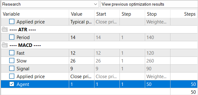
We did not reduce the replay buffer of the experience as a whole. But at the same time, there is no need for a database of 1.3M states to perform 10K iterations of updating model parameters. Of course, a larger database allows us to better tune the model. But when there are more than 100 states per update iteration, we are not able to work through them all. Therefore, we will fill the experience playback buffer gradually. At the first iteration, we launch the training data collection EA for only 50 passes. This already gives us about 120K states for training models on the specified historical period.
After the first iteration of model training, we supplement the database of examples with another 50 passes. Thus, we gradually fill the experience replay buffer with new states that correspond to the actions of the Actor within the framework of the trained policy.
This approach significantly increases the manual labor involved in launching EAs. But this allows us to keep the database of examples relatively up to date. The generated internal reward will direct the Actor to explore new environment states.
While training the models, we managed to obtain a model capable of generating profit on the training sample and generalizing the acquired knowledge for subsequent environmental states. For example, in the strategy tester, the model we trained was able to generate a profit of 1% within a month following the training sample. During the testing period, the model performed 133 trading operations, 42% of which were closed with a profit. The maximum profit per trade is almost 2 times higher than the maximum losing trade. The average profit per trade is 40% higher than the average loss. All this together allowed us to obtain a profit factor of 1.02.


Conclusion
In this article, I have introduced a new approach to encouraging exploration in reinforcement learning based on nuclear norm maximization. This method allows us to effectively assess the novelty of environmental research, taking into account historical information and ensuring high tolerance to noise and emissions.
In the practical part of the article, we integrated the Nuclear Norm Maximization method into the RE3 algorithm. We trained the model and tested it in the MetaTrader 5 strategy tester. Based on the test results, we can say that the proposed method significantly diversified the behavior of the Actor compared to the results of training the model using the pure RE3 method. However, we ended up with more chaotic trading. This may indicate the need to work out the balance between exploration and exploitation by introducing additional influence ratios into the reward function.
Links
- Nuclear Norm Maximization Based Curiosity-Driven Learning
- Neural networks made easy (Part 53): Reward decomposition
- Neural networks made easy (Part 54): Using random encoder for efficient research (RE3)
Programs used in the article
| # | Name | Type | Description |
|---|---|---|---|
| 1 | Research.mq5 | Expert Advisor | Example collection EA |
| 2 | Study.mq5 | Expert Advisor | Agent training EA |
| 3 | Test.mq5 | Expert Advisor | Model testing EA |
| 4 | Trajectory.mqh | Class library | System state description structure |
| 5 | NeuroNet.mqh | Class library | A library of classes for creating a neural network |
| 6 | NeuroNet.cl | Code Base | OpenCL program code library |
Translated from Russian by MetaQuotes Ltd.
Original article: https://www.mql5.com/ru/articles/13242
Warning: All rights to these materials are reserved by MetaQuotes Ltd. Copying or reprinting of these materials in whole or in part is prohibited.
This article was written by a user of the site and reflects their personal views. MetaQuotes Ltd is not responsible for the accuracy of the information presented, nor for any consequences resulting from the use of the solutions, strategies or recommendations described.

- Free trading apps
- Over 8,000 signals for copying
- Economic news for exploring financial markets
You agree to website policy and terms of use