Neural networks made easy (Part 50): Soft Actor-Critic (model optimization)

MetaTrader 5 — Trading systems | 17 November 2023, 10:32

3 139

Dmitriy Gizlyk

Introduction

We continue to study the Soft Actor-Critic algorithm. In the previous article, we implemented the algorithm but were unable to train a profitable model. Today we will consider possible solutions. A similar question has already been raised in the article "Model procrastination, reasons and solutions". I propose to expand our knowledge in this area and consider new approaches using our Soft Actor-Critic model as an example.

1. Model optimization

Before we move directly to optimizing the model we built, let me remind you that Soft Actor-Critic is a reinforcement learning algorithm for stochastic models in a continuous action space. The main feature of this method is the introduction of an entropy component into the reward function.

Using a stochastic Actor policy allows the model to be more flexible and capable of solving problems in complex environments where some actions may be uncertain or incapable of defining clear rules. This policy is often more robust when dealing with data containing a lot of noise since it takes into account the probabilistic component and is not tied to clear rules.

Adding an entropy component encourages exploration of the environment increasing the reward of low probability actions. The balance between exploration and exploitation is governed by the temperature ratio.

In mathematical form, the Soft Actor-Critic method can be represented by the following equation.

SAC mathematical representation

1.1 Adding stochasticity to the Actor policy

In our implementation, we abandoned the use of the stochastic Actor policy due to the complexity of its implementation using OpenCL. Similar to TD3, we replaced it with a random offset of the selected action in some of its surroundings. This approach is easier to implement and allows the model to explore the environment. But it also has its disadvantages.

The first thing that draws attention is the lack of connection between the sampled action and the distribution learned by the model. In some cases, when the learned distribution is wider than the sampling area, this compresses the study area. This means that the model policy is most likely not optimal, but depends on a randomly selected starting point of learning. After all, when initializing a new model, we fill it with random weights.

In other cases, the sampled action may fall outside the learned distribution. This expands the scope of research, but conflicts with the entropy component of the reward function. From the point of view of the model, an action outside the learned distribution has zero probability. It receives the maximum reward regardless of its value, thanks to the entropy component.

During training, the model strives to find a profitable strategy and increases the likelihood of actions with the maximum reward. At the same time, the likelihood of less profitable and unprofitable actions is reduced. The simple sampling we used earlier does not take this factor into account. It will provide us with any action from the sampling area with equal probability. The low probability of unprofitable actions generates a high entropy component. This distorts the true value of actions, neutralizes previously accumulated experience and leads to the construction of an incorrect Actor policy.

There is only one solution here - building a stochastic model of the actor and sampling actions from the learned distribution.

We have already talked about the lack of a pseudorandom number generator on the OpenCL context side, so we will use the generator on the side of the main program.

At the same time, we remember that the learned distribution is available only on the OpenCL side. It is contained in the internal objects of our model. Therefore, to arrange the sampling process, we have to implement data transfer between the main program and the OpenCL context. This does not depend on where the process is arranged.

When organizing the process on the main program side, we need to load the distribution. This involves 2 buffers: probabilities and corresponding function values.

When arranging a process on the OpenCL context side, we have to pass a buffer of random values. It will later be used to select a separate action.

Here one more point should be taken into account - the consumer of the obtained values. During operation, we will use sampled values to perform actions, i.e. on the main program side. But during training, we will transfer them to the Critic on the OpenCL side of the context. As we know, the model training imposes the most strict requirements for reducing the time for performing operations. Considering this, the decision to transfer only one buffer of random values to the OpenCL context and arrange further sampling process there seems quite logical.

The decision has been made, let's begin implementation. First, we modify the SAC_AlphaLogProbs kernel of the OpenCL program. Our changes will even simplify the algorithm of the specified kernel to some extent.

We add one buffer of random values in the external parameters of the kernel. We expect to receive a set of random values in the range [0, 1] to arrange the sampling process in this buffer.

__kernel void SAC_AlphaLogProbs(__global float *outputs,
                                __global float *quantiles,
                                __global float *probs,
                                __global float *alphas,
                                __global float *log_probs,
                                __global float *random,
                                const int count_quants,
                                const int activation
                               )
  {
   const int i = get_global_id(0);
   int shift = i * count_quants;
   float prob = 0;
   float value = 0;
   float sum = 0;
   float rnd = random[i];

To select an action, we arrange a loop of enumerating the probabilities of all quantiles of the action being analyzed and calculating their cumulative sum. In the body of the loop, while simultaneously calculating the cumulative sum, we also check its current value with the resulting random value. As soon as it exceeds this value, we use the current quantile as the selected action and interrupt the execution of the loop iterations.

   for(int r = 0; r < count_quants; r++)
     {
      prob = probs[shift + r];
      sum += prob;
      if(sum >= rnd || r == (count_quants - 1))
        {
         value = quantiles[shift + r];
         break;
        }
     }

Now we do not need to look for the nearest pair of quantiles, as we did before. We have one selected quantile with a known probability. All we have to do is activate the resulting value and calculate the value of the entropy component.

   switch(activation)
     {
      case 0:
         outputs[i] = tanh(value);
         break;
      case 1:
         outputs[i] = 1 / (1 + exp(-value));
         break;
      case 2:
         if(value < 0)
            outputs[i] = value * 0.01f;
         else
            outputs[i] = value;
         break;
      default:
         outputs[i] = value;
         break;
     }
   log_probs[i] = -alphas[i] * log(prob);
  }

After making changes to the kernel, we will supplement the code of the main program. We will start by making changes to the CNeuronSoftActorCritic class. Here we add a buffer for random values. Its initialization occurs in the Init method, similar to the cLogProbs buffer. I will not dwell on this. There is no need to save it, since it is filled anew with each direct pass. Therefore, we do not make any adjustments to the file processing methods.

class CNeuronSoftActorCritic  :  public CNeuronFQF
  {
protected:
..........
..........
   CBufferFloat         cRandomize;
..........
..........
  };

Let's turn to the forward pass method CNeuronSoftActorCritic::feedForward. Here, after a direct pass through the parent class and the inner cAlphas layer, we arrange a loop by the number of actions and fill the cRandomize buffer with random values.

bool CNeuronSoftActorCritic::feedForward(CNeuronBaseOCL *NeuronOCL)
  {
   if(!CNeuronFQF::feedForward(NeuronOCL))
      return false;
   if(!cAlphas.FeedForward(GetPointer(cQuantile0), cQuantile2.getOutput()))
      return false;
//---
   int actions = cRandomize.Total();
   for(int i = 0; i < actions; i++)
     {
      float probability = (float)MathRand() / 32767.0f;
      cRandomize.Update(i, probability);
     }
   if(!cRandomize.BufferWrite())
      return false;

The data of the filled buffer are passed to the OpenCL context memory.

Next, we implement placing the kernel into the execution queue. Here we need to transfer the parameters added to the kernel.

   uint global_work_offset[1] = {0};
   uint global_work_size[1] = {Neurons()};
   if(!OpenCL.SetArgumentBuffer(def_k_SAC_AlphaLogProbs, def_k_sac_alp_alphas, cAlphas.getOutputIndex()))
     {
      printf("Error of set parameter kernel %s: %d; line %d", __FUNCTION__, GetLastError(), __LINE__);
      return false;
     }
   if(!OpenCL.SetArgumentBuffer(def_k_SAC_AlphaLogProbs, def_k_sac_alp_log_probs, cLogProbs.GetIndex()))
     {
      printf("Error of set parameter kernel %s: %d; line %d", __FUNCTION__, GetLastError(), __LINE__);
      return false;
     }
   if(!OpenCL.SetArgumentBuffer(def_k_SAC_AlphaLogProbs, def_k_sac_alp_outputs, getOutputIndex()))
     {
      printf("Error of set parameter kernel %s: %d; line %d", __FUNCTION__, GetLastError(), __LINE__);
      return false;
     }
   if(!OpenCL.SetArgumentBuffer(def_k_SAC_AlphaLogProbs, def_k_sac_alp_probs, cSoftMax.getOutputIndex()))
     {
      printf("Error of set parameter kernel %s: %d; line %d", __FUNCTION__, GetLastError(), __LINE__);
      return false;
     }
   if(!OpenCL.SetArgumentBuffer(def_k_SAC_AlphaLogProbs, def_k_sac_alp_quantiles, 
                                                                            cQuantile2.getOutputIndex()))
     {
      printf("Error of set parameter kernel %s: %d; line %d", __FUNCTION__, GetLastError(), __LINE__);
      return false;
     }
   if(!OpenCL.SetArgumentBuffer(def_k_SAC_AlphaLogProbs, def_k_sac_alp_random, cRandomize.GetIndex()))
     {
      printf("Error of set parameter kernel %s: %d; line %d", __FUNCTION__, GetLastError(), __LINE__);
      return false;
     }
   if(!OpenCL.SetArgument(def_k_SAC_AlphaLogProbs, def_k_sac_alp_count_quants, 
                                                        (int)(cSoftMax.Neurons() / global_work_size[0])))
     {
      printf("Error of set parameter kernel %s: %d; line %d", __FUNCTION__, GetLastError(), __LINE__);
      return false;
     }
   if(!OpenCL.SetArgument(def_k_SAC_AlphaLogProbs, def_k_sac_alp_activation, (int)activation))
     {
      printf("Error of set parameter kernel %s: %d; line %d", __FUNCTION__, GetLastError(), __LINE__);
      return false;
     }
   if(!OpenCL.Execute(def_k_SAC_AlphaLogProbs, 1, global_work_offset, global_work_size))
     {
      printf("Error of execution kernel %s: %d", __FUNCTION__, GetLastError());
      return false;
     }
//---
   return true;
  }

Thus, we have implemented the stochasticity of the choice of action during the forward passage of our Actor. But there is a nuance concerning the reverse passage. The point is that the backward pass should distribute the error gradient to each decision element according to its contribution. Previously, we used a direct pass of the parent class and the error gradient was distributed similarly. Now we have made adjustments at the final stage of action selection. Consequently, this should also be reflected in the distribution of the error gradient.

Generating random values is beyond the scope of our model, and we will not distribute a gradient on them. But we should arrange the distribution of the error gradient only for the selected action. After all, none of the other values had an impact on the performed Actor's action. Therefore, their error gradient is "0".

Unlike the direct pass, we cannot add a new method to the functionality, because calling the parent class method will overwrite the gradients we have saved. Therefore, we have to completely redefine the method of distributing error gradients through the elements of our neural layer.

As always, we start by creating the SAC_OutputGradient kernel. The structure of kernel parameters will remind you of the FQF_OutputGradient kernel of the parent class. We took it as a basis and added 1 buffer and 2 constants:

output — buffer of forward pass results
count_quants — number of quantiles for each action
activation — applied activation function.

__kernel void SAC_OutputGradient(__global float* quantiles,
                                 __global float* delta_taus,
                                 __global float* output_gr,
                                 __global float* quantiles_gr,
                                 __global float* taus_gr,
                                 __global float* output,
                                 const int count_quants,
                                 const int activation
                                )
  {
   size_t action = get_global_id(0);
   int shift = action * count_quants;

We will launch the kernel in a one-dimensional task space according to the number of actions.

In the kernel body, we immediately identify the Actor’s action being analyzed and determine the offset in the data buffers.

Next, we arrange a loop in which we will compare the average value of each quantile and the perfect action from the results buffer of our layer. However, we should keep in mind that the average quantile values are stored in the original value, and the selected action in the result buffer contains the value after the activation function. Therefore, before comparing values, we need to apply an activation function to the mean of each quantile.

   for(int i = 0; i < count_quants; i++)
     {
      float quant = quantiles[shift + i];
      switch(activation)
        {
         case 0:
            quant = tanh(quant);
            break;
         case 1:
            quant = 1 / (1 + exp(-quant));
            break;
         case 2:
            if(quant < 0)
               quant = quant * 0.01f;
            break;
        }
      if(output[i] == quant)
        {
         float gradient = output_gr[action];
         quantiles_gr[shift + i] = gradient * delta_taus[shift + i];
         taus_gr[shift + i] = gradient * quant;
        }
      else
        {
         quantiles_gr[shift + i] = 0;
         taus_gr[shift + i] = 0;
        }
     }
  }

It should be noted that theoretically we could execute the inverse function once and determine the value of the result buffer before the activation function. However, due to the error within the accuracy of the calculations, we will most likely receive a value that is close, but different from the original one. We will be forced to make a comparison with some kind of tolerance. This in turn will complicate the comparison and reduce accuracy.

When a quantile matches, we distribute the error gradient to the mean of the quantile and its probability. For the remaining quantiles and their probabilities, we set the gradient to "0".

After completing the loop iterations, we shut down the kernel.

As mentioned above, on the side of the main program, we have to completely redefine the error gradient distribution method calcInputGradients. The method was copied from the similar parent class method. The changes affected only the queuing block described above the kernel. Therefore, I will not dwell on its description now. Find it in the attached file "..\NeuroNet_DNG\NeuroNet.mqh".

1.2 Adjusting the process of updating target models

You may have noticed that I prefer using the Adam method in my models to update the weighting ratios. In this regard, the idea of introducing this method into the soft update of critics' target models arose.

As you might remember, the Soft Actor-Critic algorithm provides soft update of target models using a constant ratio in the range (0, 1}. If the ratio is equal to "1", the parameters are simply copied. "0" is not applied since the target model is not updated in this case.

Using the Adam method allows the model to independently adjust the ratios for each individual trained parameter. This will make it possible to quickly update parameters that are shifted in one direction, which means that the target model will shift faster from the initial values to the first approximation. At the same time, the adaptive method makes it possible to reduce the copying speed for multidirectional oscillations, which will reduce the noise in the values of the target models.

However, attention should be paid to the risk of models becoming unbalanced at the initial stage of training. Significant differences in the speed of copying individual parameters can lead to unexpected and unpredictable results.

Having assessed all the pros and cons, I decided to test the effectiveness of this approach in practice.

We carry out the model optimization process on the OpenCL context side. The current values of all trained model parameters are stored in the context memory. It is quite logical that it is more profitable for us to transfer these parameters between the trained and target models on the OpenCL side. This approach has multiple advantages:

we eliminate the process of loading current parameters of the trained model from the context into the main memory and subsequent copying of new parameters of the target models into the context memory;
we can transfer several parameters simultaneously in parallel data streams.

Let's create the SoftUpdateAdam kernel to transfer data. In the kernel parameters, we will pass pointers to 4 data buffers and 3 parameters provided by the method.

__kernel void SoftUpdateAdam(__global float *target,
                             __global const float *source,
                             __global float *matrix_m,
                             __global float *matrix_v,
                             const float tau,
                             const float b1,
                             const float b2
                            )
  {
   const int i = get_global_id(0);
   float m, v, weight;

We plan to launch the kernel sequentially for each neural layer in the one-dimensional task space according to the number of updated parameters of the current model layer. In this option, the thread ID defined in the kernel body simultaneously serves as a pointer to the parameter being analyzed and the offset in the data buffers.

Here we also declare local variables to store intermediate data and write the original data from global buffers into them.

   m = matrix_m[i];
   v = matrix_v[i];
   weight=target[i];

The Adam method was developed to update the model parameters towards the anti-gradient. In our case, the error gradient will be the deviation of the parameters of the target model from the trained one. Since we adjust the value of the parameters towards the anti-gradient, we define the deviation as the difference between the parameter of the trained model and the corresponding parameter of the trained model.

   float g = source[i] - weight;
   m = b1 * m + (1 - b1) * g;
   v = b2 * v + (1 - b2) * pow(g, 2);

Besides, we immediately determine the exponential average of the error gradient of its quadratic value.

Next, we determine the required parameter offset and store its corresponding element in the global data buffer.

   float delta = tau * m / (v != 0.0f ? sqrt(v) : 1.0f);
   if(delta * g > 0)
      target[i] = clamp(weight + delta, -MAX_WEIGHT, MAX_WEIGHT);

At the end of the kernel operations, we save the average values of the error gradient and its square into global data buffers. We will need them in subsequent iterations of updating parameters.

   matrix_m[i] = m;
   matrix_v[i] = v;
  }

After creating the kernel, we have to arrange the process of calling it on the side of the main program. Here we have 2 options:

creating a new method
updating a previously created method.

In this article, I propose creating a new method, which we will create at the level of the base class of the CNeuronBaseOCL::WeightsUpdateAdam neural layer. In the method parameters, we will pass a pointer to the neural layer of the trained model and the update coefficient, similar to the previously created soft update method of the target model. We will use the Adam method hyperparameters specified to update the default models.

bool CNeuronBaseOCL::WeightsUpdateAdam(CNeuronBaseOCL *source, float tau)
  {
   if(!OpenCL || !source)
      return false;
   if(Type() != source.Type())
      return false;
   if(!Weights || Weights.Total() == 0)
      return true;
   if(!source.Weights || Weights.Total() != source.Weights.Total())
      return false;

The block of controls will be implemented in the method body. Here we check the relevance of pointers to the objects being used. We also check the correspondence between the type of the current neural layer and the resulting pointer.

After successfully passing the control block, we transfer parameters to the kernel and put it in the execution queue.

Please note here that the Adam method requires the creation of two additional data buffers. But let's remember that we create similar buffers in each model to update the model's trainable parameters. In this case, we are dealing with the target model, in which the parameters are updated. Its optimization is carried out by periodically transferring data from the trained model. In other words, we have a model with limited functionality. At the same time, we did not create separate types of objects for target models, but used previously created ones for fully functional models with the creation of all necessary objects and buffers. This can be seen as inefficient use of memory resources. But we consciously took this step in order to unify the models. Now we have created and unused target model buffers. We will use them to update the parameters.

   uint global_work_offset[1] = {0};
   uint global_work_size[1] = {Weights.Total()};
   ResetLastError();
   if(!OpenCL.SetArgumentBuffer(def_k_SoftUpdateAdam, def_k_sua_target, getWeightsIndex()))
     {
      printf("Error of set parameter kernel %s: %d; line %d", __FUNCTION__, GetLastError(), __LINE__);
      return false;
     }
   if(!OpenCL.SetArgumentBuffer(def_k_SoftUpdateAdam, def_k_sua_source, source.getWeightsIndex()))
     {
      printf("Error of set parameter kernel %s: %d; line %d", __FUNCTION__, GetLastError(), __LINE__);
      return false;
     }
   if(!OpenCL.SetArgumentBuffer(def_k_SoftUpdateAdam, def_k_sua_matrix_m, getFirstMomentumIndex()))
     {
      printf("Error of set parameter kernel %s: %d; line %d", __FUNCTION__, GetLastError(), __LINE__);
      return false;
     }
   if(!OpenCL.SetArgumentBuffer(def_k_SoftUpdateAdam, def_k_sua_matrix_v, getSecondMomentumIndex()))
     {
      printf("Error of set parameter kernel %s: %d; line %d", __FUNCTION__, GetLastError(), __LINE__);
      return false;
     }
   if(!OpenCL.SetArgument(def_k_SoftUpdateAdam, def_k_sua_tau, (float)tau))
     {
      printf("Error of set parameter kernel %s: %d; line %d", __FUNCTION__, GetLastError(), __LINE__);
      return false;
     }
   if(!OpenCL.SetArgument(def_k_SoftUpdateAdam, def_k_sua_b1, (float)b1))
     {
      printf("Error of set parameter kernel %s: %d; line %d", __FUNCTION__, GetLastError(), __LINE__);
      return false;
     }
   if(!OpenCL.SetArgument(def_k_SoftUpdateAdam, def_k_sua_b2, (float)b2))
     {
      printf("Error of set parameter kernel %s: %d; line %d", __FUNCTION__, GetLastError(), __LINE__);
      return false;
     }
   if(!OpenCL.Execute(def_k_SoftUpdateAdam, 1, global_work_offset, global_work_size))
     {
      printf("Error of execution kernel %s: %d", __FUNCTION__, GetLastError());
      return false;
     }
//---
   return true;
  }

Do not forget to monitor the correctness of operations at each stage. Complete the method after successful completion of all iterations.

After creating a method, we need to think through and arrange its calling. I wanted to find an approach that would make calling it as simple as possible with a minimum number of changes in the overall structure of the models. It seems to me that I have found a compromise. I did not create a separate branch for calling a method from an external program through the dispatcher class of the model and the dynamic array of neural layers. Instead, I went into the previously created CNeuronBaseOCL::WeightsUpdate soft update method and set up a check for the method for updating the trained model parameters, which is specified by the user for each neural layer when describing the model architecture. If the user specified the Adam method to update the model parameters, we simply redirect the workflow to execute our new method. For other parameter update methods, we use classic soft update.

bool CNeuronBaseOCL::WeightsUpdate(CNeuronBaseOCL *source, float tau)
  {
   if(optimization == ADAM)
      return WeightsUpdateAdam(source, tau);
//---
........
........
  }

Among other things, this approach guarantees that we have the necessary data buffers.

1.3 Making changes to the source data structure

I also paid attention to the source data structure. As you know, the description of each historical data bar consists of 12 elements:

difference between opening and closing prices
difference between opening and maximum prices
difference between opening and minimum prices
candle hour
week day
month
5 indicator parameters.

      State.Add((float)Rates[b].close - open);
      State.Add((float)Rates[b].high - open);
      State.Add((float)Rates[b].low - open);
      State.Add((float)Rates[b].tick_volume / 1000.0f);
      State.Add((float)sTime.hour);
      State.Add((float)sTime.day_of_week);
      State.Add((float)sTime.mon);
      State.Add(rsi);
      State.Add(cci);
      State.Add(atr);
      State.Add(macd);
      State.Add(sign);

In this dataset, my attention was drawn to the timestamps. Assessing the time component is of great value in understanding seasonality and the different behavior of currencies in different sessions. But how important is their presence for each candle? My personal opinion is that one set of timestamps is enough for an overall set of "snapshots" of the current state of the market. Previously, when using one buffer of source data, we were forced to repeat this data in order to preserve the structure of the description of each candle. Now, when our models have 2 sources of initial data, we can put timestamps into the account state description buffer. Here we leave only historical data of a market situation snapshot. In this way, we reduce the total volume of analyzed data without losing information capacity. Consequently, we reduce the number of operations performed, while increasing the performance of our model.

Additionally, we changed the representation of timestamps for our model. Let me remind you that we use relative parameters to describe the state of the account. This allows us to bring them into a comparable and partly normalized form. We would like to have a normalized view of timestamps. At the same time, it is important to preserve information about the seasonality of processes. In such cases, one often comes to use the sine and cosine functions. The graphs of these functions are continuous and cyclic. The length of the function cycle is known and equal to 2π.

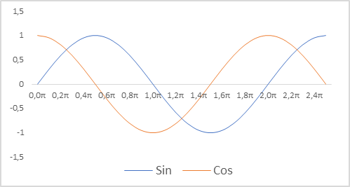
To normalize the timestamp and take the cyclical nature into account, we need to:

Divide the current time by the period size
Multiply the resulting value by the "2π" constant
Calculate the function value (sin or cos)
Add the resulting value to the buffer

In my implementation, I used the periods of year, month, week and day.

   double x = (double)Rates[0].time / (double)(D'2024.01.01' - D'2023.01.01');
   Account.Add((float)MathSin(x != 0 ? 2.0 * M_PI * x : 0));
   x = (double)Rates[0].time / (double)PeriodSeconds(PERIOD_MN1);
   Account.Add((float)MathCos(x != 0 ? 2.0 * M_PI * x : 0));
   x = (double)Rates[0].time / (double)PeriodSeconds(PERIOD_W1);
   Account.Add((float)MathSin(x != 0 ? 2.0 * M_PI * x : 0));
   x = (double)Rates[0].time / (double)PeriodSeconds(PERIOD_D1);
   Account.Add((float)MathSin(x != 0 ? 2.0 * M_PI * x : 0));

Also, do not forget to change the size constants for the description of one candle and the account state. Their values will be reflected in the architecture of our model and the sizes of the arrays as a buffer for describing the trajectories of accumulated experience.

#define                    BarDescr        9            //Elements for 1 bar description
#define                    AccountDescr   12            //Account description

It is worth noting that the preparation of source data, and normalization of timestamps in particular, is not related to the construction of the model itself and its architecture. It is carried out on the side of an external program. But the quality of source data preparation greatly affects the model training process and result.

2. Model training

After making constructive changes to the model work, it is time to move on to training. At the first stage, we use the "..\SoftActorCritic\Research.mq5" EA to interact with the environment and collect data into the training set.

In the specified EA, we make the changes described above to transfer time stamps from the environment state buffer to the account state buffer.

//+------------------------------------------------------------------+
//| Expert tick function                                             |
//+------------------------------------------------------------------+
void OnTick()
  {
//---
.........
.........
//---
   float atr = 0;
   for(int b = 0; b < (int)HistoryBars; b++)
     {
      float open = (float)Rates[b].open;
      float rsi = (float)RSI.Main(b);
      float cci = (float)CCI.Main(b);
      atr = (float)ATR.Main(b);
      float macd = (float)MACD.Main(b);
      float sign = (float)MACD.Signal(b);
      if(rsi == EMPTY_VALUE || cci == EMPTY_VALUE || atr == EMPTY_VALUE || macd == EMPTY_VALUE || sign == EMPTY_VALUE)
         continue;
      //---
      int shift = b * BarDescr;
      sState.state[shift] = (float)(Rates[b].close - open);
      sState.state[shift + 1] = (float)(Rates[b].high - open);
      sState.state[shift + 2] = (float)(Rates[b].low - open);
      sState.state[shift + 3] = (float)(Rates[b].tick_volume / 1000.0f);
      sState.state[shift + 4] = rsi;
      sState.state[shift + 5] = cci;
      sState.state[shift + 6] = atr;
      sState.state[shift + 7] = macd;
      sState.state[shift + 8] = sign;
     }
   State.AssignArray(sState.state);
//---
........
........
//---
   Account.Clear();
   Account.Add((float)((sState.account[0] - PrevBalance) / PrevBalance));
   Account.Add((float)(sState.account[1] / PrevBalance));
   Account.Add((float)((sState.account[1] - PrevEquity) / PrevEquity));
   Account.Add(sState.account[2]);
   Account.Add(sState.account[3]);
   Account.Add((float)(sState.account[4] / PrevBalance));
   Account.Add((float)(sState.account[5] / PrevBalance));
   Account.Add((float)(sState.account[6] / PrevBalance));
   double x = (double)Rates[0].time / (double)(D'2024.01.01' - D'2023.01.01');
   Account.Add((float)MathSin(x != 0 ? 2.0 * M_PI * x : 0));
   x = (double)Rates[0].time / (double)PeriodSeconds(PERIOD_MN1);
   Account.Add((float)MathCos(x != 0 ? 2.0 * M_PI * x : 0));
   x = (double)Rates[0].time / (double)PeriodSeconds(PERIOD_W1);
   Account.Add((float)MathSin(x != 0 ? 2.0 * M_PI * x : 0));
   x = (double)Rates[0].time / (double)PeriodSeconds(PERIOD_D1);
   Account.Add((float)MathSin(x != 0 ? 2.0 * M_PI * x : 0));
//---
   if(Account.GetIndex() >= 0)
      if(!Account.BufferWrite())
         return;

In addition, I decided to abandon hedging operations. A deal is opened only for the difference in volumes in the direction of the larger one. To do this, we check the forecast volumes of transactions and reduce their volume.

........
........
//---
   vector<float> temp;
   Actor.getResults(temp);
   float delta = MathAbs(ActorResult - temp).Sum();
   ActorResult = temp;
//---
   if(temp[0] >= temp[3])
     {
      temp[0] -= temp[3];
      temp[3] = 0;
     }
   else
     {
      temp[3] -= temp[0];
      temp[0] = 0;
     }

In addition, I paid attention to the reward generated. When forming the main body of the reward, we used the relative change in the account balance. Its value is rarefied and significantly below 1. At the same time, the value of the entropy component of reward at the initial training stage fluctuated in the range of 8-12. It is obvious that the size of the entropy component is incomparably large. To compensate for this gap in values, I divided it by the balance amount, as is done with its change when forming the target part of the reward. Besides, I additionally introduced the LogProbMultiplier reduction ratio.

........
........
//---
   float reward = Account[0];
   if((buy_value + sell_value) == 0)
      reward -= (float)(atr / PrevBalance);
   for(ulong i = 0; i < temp.Size(); i++)
      sState.action[i] = temp[i];
   if(Actor.GetLogProbs(temp))
      reward += LogProbMultiplier * temp.Sum() / (float)PrevBalance;
   if(!Base.Add(sState, reward))
      ExpertRemove();
  }

After making these changes, I started the first stage of collecting training data. To do this, I used historical data on EURUSD H1. Data collection was carried out in the strategy tester for the first 5 months of 2023 in the full parameter enumeration mode. The starting capital is USD 10,000. At this stage, I collected a sample database of 200 passes, which gives us more than 0.5 million "State"→"Action"→"New state"→"Reward" data sets over the specified time interval.

As you might remember, we do not have a pre-trained model at this stage. With each pass, the EA generates a new model and fills it with random parameters. During the passage through history, model training is not carried out. Therefore, we get 200 completely random and independent passes. None of them showed a profit.

First data collection

The actual process of training the model is organized in the "..\SoftActorCritic\Study.mq5" EA. We also made some spot edits here.

First, we made changes to the process of generating the account state description vector in terms of adding timestamps similar to the approach described above in the environment research EA.

In addition, we adjusted the formation of the target reward in terms of the entropy component. The approach should be the same in all three EAs.

void Train(void)
  {
.........
.........
//---
   for(int iter = 0; (iter < Iterations && !IsStopped()); iter ++)
     {
.........
.........
      Account.Clear();
      Account.Add((Buffer[tr].States[i + 1].account[0] - PrevBalance) / PrevBalance);
      Account.Add(Buffer[tr].States[i + 1].account[1] / PrevBalance);
      Account.Add((Buffer[tr].States[i + 1].account[1] - PrevEquity) / PrevEquity);
      Account.Add(Buffer[tr].States[i + 1].account[2]);
      Account.Add(Buffer[tr].States[i + 1].account[3]);
      Account.Add(Buffer[tr].States[i + 1].account[4] / PrevBalance);
      Account.Add(Buffer[tr].States[i + 1].account[5] / PrevBalance);
      Account.Add(Buffer[tr].States[i + 1].account[6] / PrevBalance);
      double x = (double)Buffer[tr].States[i + 1].account[7] / (double)(D'2024.01.01' - D'2023.01.01');
      Account.Add((float)MathSin(x != 0 ? 2.0 * M_PI * x : 0));
      x = (double)Buffer[tr].States[i + 1].account[7] / (double)PeriodSeconds(PERIOD_MN1);
      Account.Add((float)MathCos(x != 0 ? 2.0 * M_PI * x : 0));
      x = (double)Buffer[tr].States[i + 1].account[7] / (double)PeriodSeconds(PERIOD_W1);
      Account.Add((float)MathSin(x != 0 ? 2.0 * M_PI * x : 0));
      x = (double)Buffer[tr].States[i + 1].account[7] / (double)PeriodSeconds(PERIOD_D1);
      Account.Add((float)MathSin(x != 0 ? 2.0 * M_PI * x : 0));
      //---
.........
.........
      //---
      TargetCritic1.getResults(Result);
      float reward = Result[0];
      TargetCritic2.getResults(Result);
      reward = Buffer[tr].Revards[i] + DiscFactor * (MathMin(reward, Result[0]) - Buffer[tr].Revards[i + 1] + 
                                                     LogProbMultiplier * log_prob.Sum() / (float)PrevBalance);

We then separated the training of the Actor and the Critic. As before, we alternate Critic1 and Critic2 in the even and odd training iterations. But now, when training an Actor, we disable the training functionality of the Critic being used. It only passes the error gradient to the Actor. In this case, Critic parameters are not updated. Thus, we aim to train an objective Critic on real environment rewards.

........
........
      //---
      if((iter % 2) == 0)
        {
         if(!Critic1.feedForward(GetPointer(Actor), LatentLayer, GetPointer(Actor)) ||
            !Critic2.feedForward(GetPointer(Actor), LatentLayer, GetPointer(Actions)))
           {
            PrintFormat("%s -> %d", __FUNCTION__, __LINE__);
            break;
           }
         Critic1.getResults(Result);
         Actor.GetLogProbs(log_prob);
         Result.Update(0, reward);
         Critic1.TrainMode(false);
         if(!Critic1.backProp(Result, GetPointer(Actor)) ||
            !Critic1.AlphasGradient(GetPointer(Actor)) ||
            !Actor.backPropGradient(GetPointer(Account), GetPointer(Gradient), LatentLayer) ||
            !Actor.backPropGradient(GetPointer(Account), GetPointer(Gradient)))
           {
            PrintFormat("%s -> %d", __FUNCTION__, __LINE__);
            Critic1.TrainMode(true);
            break;
           }
         Critic1.TrainMode(true);

In addition, when training a critic, we exclude the entropy component from the target reward since we need an objective Critic, while the function of the entropy component is to stimulate the Actor to explore the environment.

         Result.Update(0, reward - LogProbMultiplier * log_prob.Sum() / (float)PrevBalance);
         if(!Critic2.backProp(Result, GetPointer(Actions), GetPointer(Gradient)))
           {
            PrintFormat("%s -> %d", __FUNCTION__, __LINE__);
            break;
           }
         //--- Update Target Nets
         TargetCritic2.WeightsUpdate(GetPointer(Critic2), Tau);
        }

After updating the Critic parameters, we update the target model of only one Critic. Otherwise, the EA code remains unchanged, and you can view it in the attachment.

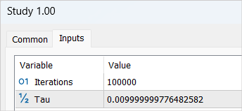
After making changes, we start the model training process with a cycle of 100,000 iterations (default parameters). At this stage, the Actor and 2 Critics models are formed. Their initial training is also carried out.

You should not expect significant results from the first round of model training. There are a number of reasons for this. The completed number of iterations covers only 1/5 of our example base. It cannot be called complete. There is not a single profitable passage in it the model can learn.

After completing the first stage of the model training, I deleted the previously collected example database. My logic here is pretty simple. This database contains random independent passes. The rewards contain the unknown entropy component. I assume that in an untrained model all actions are equally likely. But in any case, they will not be comparable with the probability distribution of our model. Therefore, we delete the previously collected database of examples and create a new one.

At the same time, we repeat the process of collecting a training sample and re-run the optimization of the environmental research EA with a complete search of parameters. Only this time we shift the value of the Agents being iterated. This simple trick is necessary to avoid loading data from the previous optimization cache.

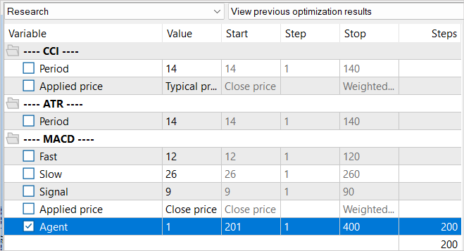
The main difference between the new example base is that our pre-trained model was used during the environmental exploration process. The diversity of the Agent's actions is due to the stochasticity of the Actor’s policy. And all completed actions lie within the learned probability distribution of our model. At this stage, we collect all of our Agent's passes for the last time.

After collecting a new database of examples, we re-run the "..\SoftActorCritic\Study.mq5" model training EA. This time we increase the number of training iterations to 500,000.

After completing the second cycle of the training process, we turn to the "..\SoftActorCritic\Test.mq5" EA for testing the trained model. We are making changes to it similar to the environment research EA. You can find them in the attachment.

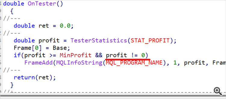
Switching to the testing EA does not mean the end of training. We run the EA several times on historical data from the training period. In my case, this is the first 5 months of 2023. I carried out 10 passes and determined the approximate upper 1/4 or 1/5 of the obtained profit range. Let's get back to the code of the environment research EA and introduce a restriction on the minimum profitability of passes saved to the example database.

input double               MinProfit   =  10;

double OnTester()
  {
//---
   double ret = 0.0;
//---
   double profit = TesterStatistics(STAT_PROFIT);
   Frame[0] = Base;
   if(profit >= MinProfit && profit != 0)
      FrameAdd(MQLInfoString(MQL_PROGRAM_NAME), 1, profit, Frame);
//---
   return(ret);
  }

Thus, we strive to select only the best passages and train our Actor on them to use the optimal strategy.

We deliberately included the minimum profitability indicator in external parameters, since we are going to gradually raise the bar while training the model.

After making changes, we set the previously determined minimum profitability level and carry out another 100 passes in the strategy tester optimization mode on training data.

We repeat iterations of the model training process until the desired results are obtained or the upper limit of the model capabilities is reached (the next training cycle does not change the profitability). This can also be noticed when performing single passes of the testing EA. In this case, despite the stochasticity of the Actor's policy, several perfect passes will have almost identical results. This is evidence that the model maximized the probability of individual actions in the relevant states. We get the effect of a deterministic strategy. This result is not always a disadvantage. A stable and deterministic strategy may be preferable in some tasks, especially if deterministic actions lead to good results.

3. Test

After about 15 iterations of updating the example database, training the model, testing on the training sample, raising the minimum profitability bar and regularly replenishing the example database, I was able to get a model that consistently generates profit on the training range of historical data.

The next stage is testing the capabilities of the trained model outside the training set on new data. I tested the performance of the trained model on historical data for June 2023. As you can see, this is the month following the training period.

During the testing period, the model made only four long trades. Only one of them was profitable. This is probably not the result we expected. But look at the balance graph. 3 losing trades resulted in a total loss of USD 300 with a starting balance of USD 10,000. At the same time, one profitable trade resulted in a profit of more than USD 2000. As a result, we have a profit of 17.5% for the month. The profit factor - 6.77, the recovery factor - 1.32 and the balance drawdown - 1.65%.

Testing the trained model

The small number of trades and their one-directional nature are confusing. But what is more important? The number of trades and their variety or the final change in the balance?

Conclusion

In this article, we resumed our work on building the Soft Actor-Critic algorithm. The additions helped us train the Actor's profitable strategy. It is difficult to say how optimal the resulting model is. Everything is relative.

The approaches proposed in the article made it possible to increase the profitability of our model, but they are not the only and exhaustive ones. For example, in the forum thread to the previous article, the user JimReaper proposed his model architecture. This is also a completely viable option. Personally, I have not tested it yet, but I fully admit the possibility of making a profit using the proposed or some other architecture. It is highly likely that adding new data for analysis by the model will help improve its efficiency. I always encourage exploration and new research. When developing and optimizing models in reinforcement learning (as in other areas of machine learning), exploring and experimenting with different architectures, hyperparameters, and new data are key elements that can lead to model optimization and improvement.

Programs used in the article

#	Name	Type	Description
1	Research.mq5	Expert Advisor	Example collection EA
2	Study.mq5	Expert Advisor	Agent training EA
3	Test.mq5	Expert Advisor	Model testing EA
4	Trajectory.mqh	Class library	System state description structure
5	NeuroNet.mqh	Class library	A library of classes for creating a neural network
6	NeuroNet.cl	Code Base	OpenCL program code library

Translated from Russian by MetaQuotes Ltd.
Original article: https://www.mql5.com/ru/articles/12998

Attached files |

Download ZIP

MQL5.zip (1721.81 KB)

Warning: All rights to these materials are reserved by MetaQuotes Ltd. Copying or reprinting of these materials in whole or in part is prohibited.