
Neural networks made easy (Part 42): Model procrastination, reasons and solutions

Introduction
In the field of reinforcement learning, neural network models often face the problem of procrastination when the learning process slows down or gets stuck. Model procrastination can have serious consequences for achieving goals and requires taking appropriate measures. In this article, we will look at the main reasons for model procrastination and propose methods for solving them.
1. Procrastination issue
One of the main reasons for model procrastination is an insufficient training environment. The model may encounter limited access to training data or insufficient resources. Solving this problem involves creating or updating the dataset, increasing the diversity of training examples and applying additional training resources, such as computing power or pre-trained models for transfer training.
Another reason for model procrastination may be the complexity of the task it should solve or using a training algorithm that requires a lot of computing resources. In this case, the solution may be to simplify the problem or algorithm, optimize computational processes and use more efficient algorithms or distributed learning.
A model may procrastinate if it lacks motivation to achieve its goals. Setting clear and relevant goals for the model, designing a reward function that incentivizes the achievement of these goals and using reinforcement techniques, such as rewards and penalties, can help solve this problem.
If the model does not receive feedback or is not updated based on new data, it may procrastinate in its development. The solution is to establish regular model update cycles based on new data and feedback, and to develop mechanisms to control and monitor learning progress.
It is important to regularly evaluate the model's progress and learning outcomes. This will help you see progress made and identify possible problems or bottlenecks. Regular assessments will allow timely adjustments to be made to the training process to avoid delays.
Providing a model varied tasks and a stimulating environment can help avoid procrastination. Variation in the tasks will help keep the model interested and motivated, and a stimulating environment, such as competition or game elements, can encourage the model's active participation and progress.
Model procrastination may happen due to insufficient updating and improvement. It is important to regularly analyze the results and iteratively improve the model based on feedback and new ideas. Gradual development of the model and visible progress can help cope with procrastination.
Providing a positive and supportive learning environment for the model is an important aspect of training reinforcement models. Research shows that positive examples lead to more effective and focused model learning. This is because the model is in search of the most optimal choice, and penalties for incorrect actions lead to a decrease in the probability of choosing erroneous actions. At the same time, positive rewards clearly indicate to the model that the choice was correct and significantly increase the likelihood of repeating such actions.
When a model receives a positive reward for a certain action, it will pay more attention to it and will be inclined to repeat that action in the future. This motivation mechanism helps the model search for and identify the most successful strategies to achieve its goals.
Finally, to effectively address the procrastination, it is necessary to analyze the reasons behind it. Identifying the specific causes of procrastination will allow you to take targeted measures to eliminate them. This may include auditing training processes, identifying bottlenecks, resource issues or suboptimal model settings.
Taking into account and adapting to changing conditions can help avoid procrastination. Periodically updating the model based on new data and changes in the learning task will help it stay relevant and effective. Additionally, taking into account factors such as new requirements or constraints will allow the model to adapt and avoid stagnation.
Setting small goals and milestones can help break a larger task down into more manageable and achievable pieces. This will help the model see progress and maintain motivation during the learning process.
To successfully overcome procrastination in a reinforcement learning model, you need to use a variety of approaches and strategies. This comprehensive approach will help the model to effectively overcome procrastination and achieve the best results in training. By combining various techniques such as improving the learning environment, setting clear goals, regularly assessing progress and using motivation, the model will be able to overcome procrastination and move forward towards achieving its learning goals.
2. Practical solution steps
After considering theory, let's now turn to the practical application of these ideas.
In the previous article, I mentioned the need for further training to minimize losing trades. However, while continuing our training, we encountered a situation where the EA did not make a single transaction during the entire training period.
This phenomenon, called "model procrastination", is a serious problem that requires our attention and solutions.

2.1. Analyzing reasons
In order to overcome model procrastination in reinforcement learning, it is important to start by analyzing the current situation and identifying the causes of this phenomenon. The analysis will help us understand why the model is not making trades and what can be adjusted to improve its performance.
Testing of the trained model is carried out using the "Test.mq5" EA, which greedily selects an agent and action. It is important to note that each subsequent launch of the EA with the same parameters and testing period will lead to the reproduction of the previous pass with high accuracy. This allows us to add control points and analyze the EA operation each time it is launched.
Adding control points and analyzing the work of the EA at each launch provides us with greater reliability and confidence in the result of training a reinforcement model. We can better understand how the model applies its knowledge and predictions to real data, and make appropriate conclusions and adjustments to improve its performance.
To evaluate the work of the scheduler, we introduce the ModelsCount vector, which will contain the number of times each agent was selected. To do this, declare the ModelsCount vector in the block of global variables:
vector<float> ModelsCount;
Then, in the OnInit function, initialize this vector with a size corresponding to the number of agents used:
//+------------------------------------------------------------------+
//| Expert initialization function                                   |
//+------------------------------------------------------------------+
int OnInit()
  {
//---
........
........
//---
   ModelsCount = vector<float>::Zeros(Models);
//---
   return(INIT_SUCCEEDED);
  }
In the OnTick function, after each forward pass of the scheduler, increase the counter of the corresponding agent in the ModelsCount vector:
//+------------------------------------------------------------------+
//| Expert tick function                                             |
//+------------------------------------------------------------------+
void OnTick()
  {
//---
   if(!IsNewBar())
      return;
//---
........
.......
//---
   if(!Schedule.feedForward(GetPointer(State1), 12, false))
      return;
   Schedule.getResults(Result);
   int model = GetAction(Result, 0, 1);
   ModelsCount[model]++;
//---
........
........
  }
Finally, when deinitializing the EA, display the calculation results in the journal:
//+------------------------------------------------------------------+
//| Expert deinitialization function                                 |
//+------------------------------------------------------------------+
void OnDeinit(const int reason)
  {
//---
   Print(ModelsCount);
   delete Result;
  }
Thus, we add functionality to count the number of selections of each agent and display the counting results to the journal when the EA is deinitialized. This allows us to evaluate the performance of the scheduler and obtain information about how often each agent was selected during the EA execution.
After adding our first control point, we launched the EA in the strategy tester without changing the parameters or testing period. The results obtained confirmed our fears. We can see that the scheduler used only one agent during the entire testing.

This observation indicates that the scheduler may be biased in favor of a particular agent, neglecting to explore other available agents. Such bias may hamper the performance of our reinforcement learning model and limit its ability to discover more effective strategies.
To solve this problem, we need to explore the reasons why the scheduler chooses to use only one agent.
Continuing to analyze the reasons for this behavior, we add two additional control points. We now focus on the dynamics of changes in model output distributions depending on changes in the state of the environment. To do this, we introduce two additional vectors: prev_scheduler and prev_actor. In these vectors we will store the results of the previous forward pass of the scheduler and agents respectively.
vector<float>        prev_scheduler;
vector<float>        prev_actor;
This will allow us to compare current distributions with previous ones and evaluate their changes. If we find that the distributions change significantly over time or in response to changes in the environment, this may indicate that the model may be too sensitive to change or unstable in its strategies.
Adding these vectors to our model allows us to obtain more detailed information about the dynamics of changing strategies and allocations, which in turn helps us understand the reasons for the preference of a particular agent and take measures to solve this problem.
As in the previous case, we initialize the vectors in the OnInit method to prepare them for data control.
//+------------------------------------------------------------------+
//| Expert initialization function                                   |
//+------------------------------------------------------------------+
int OnInit()
  {
//---
........
........
//---
   ModelsCount = vector<float>::Zeros(Models);
   prev_scheduler.Init(Models);
   prev_actor.Init(Result.Total());
//---
   return(INIT_SUCCEEDED);
  }
The actual data control is done in the OnTick method.
//+------------------------------------------------------------------+
//| Expert tick function                                             |
//+------------------------------------------------------------------+
void OnTick()
  {
//---
   if(!IsNewBar())
      return;
//---
........
........
//---
   State1.AssignArray(sState.state);
   if(!Actor.feedForward(GetPointer(State1), 12, false))
      return;
   Actor.getResults(Result);
   State1.AddArray(Result);
   if(!Schedule.feedForward(GetPointer(State1), 12, false))
      return;
   vector<float> temp;
   Schedule.getResults(Result);
   Result.GetData(temp);
   float delta = MathAbs(prev_scheduler - temp).Sum();
   int model = GetAction(Result, 0, 1);
   prev_scheduler = temp;
   Actor.getResults(Result);
   Result.GetData(temp);
   delta = MathAbs(prev_actor - temp).Sum();
   prev_actor = temp;
   ModelsCount[model]++;
//---
........
........
//---
  }
In this case, we want to evaluate how changes in the state of the environment affect the result of the model. As a result of this experiment, we expect to see a unique probability distribution at the model output for each candle in the test sample. In other words, we want to observe changes in the model’s strategies depending on changes in market conditions.
We will not log the results of the analysis as this will result in a large amount of data. Instead, we will use debug mode to watch the values change. To reduce the volume of compared values, we will only check the total deviation of the vectors.
Unfortunately, we found no deviations during the test. This means that the probability distribution of the model output remains almost the same in all environmental states.
This observation indicates that the model does not adapt to the changing environment and does not take into account differences in market conditions. There are several possible reasons for this behavior of the model and various approaches to solve them:
- Limitations of the training dataset: If the training dataset does not contain enough variety of situations, the model may not learn to respond adequately to new conditions. The solution may be to expand and diversify the training dataset to include a wider range of scenarios and changing market conditions.
- Insufficient model training: The model may not receive enough training or go through enough training epochs to adapt to different environmental conditions. In this case, increasing the training time or using additional methods, such as fine-tuning, can help the model adapt better.
- Insufficient model complexity: The model may not be complex enough to capture subtle differences in environmental states. In this case, increasing the size and complexity of the model, such as adding more layers or increasing the number of neurons, can help it better capture and handle differences in the data.
- Wrong choice of model architecture: The current model architecture may not be suitable for solving the problem of adapting to a changing environment. In such a case, revising the model's architecture can improve its ability to adapt to changes in the environment.
- Incorrect reward function: The model's reward function may not be informative enough or may not meet the required goals. In such a case, reconsidering the reward function and incorporating more relevant factors into it can help the model make smarter decisions in a changing environment.
All of these approaches require additional experimentation, testing, and tuning of the model to achieve better adaptation to a changing environment and improve its performance.
We will analyze the architecture of each layer in order to find out exactly where in our models information about changes in the state of the system is lost. In debug mode, we will check for changes in the output of each layer of our models.
We will start with the fully connected CNeuronBaseOCL layer. In this layer we will check whether information about changes in the state of the system is preserved. Next, we will check the CNeuronBatchNormOCL batch data normalization layer to ensure that it is not distorting the state change data. We will then analyze the CNeuronConvOCL convolutional layer to see how it handles system state change information. Finally, we will examine the CNeuronMultiModel multi-model fully connected layer to determine how it accounts for state changes across models.
Conducting this analysis will help us identify at what layer of the model architecture information about changes in system state is lost and which layers can be optimized or modified to improve the model's performance in adapting to a changing environment.
To control and track the output of each layer in the model, we implement the prev_output vector in the CNeuronBaseOCL class. As you might remember, this class is the base class for all other neural layer classes, and all other layers inherit from it. By adding a vector to the body of this class, we ensure its presence in all layers of the model.
class CNeuronBaseOCL    :  public CObject
  {
protected:
........
........
   vector<float>      prev_output;
In the class initialization method, we will set the vector size, which will be equal to the number of neurons in this layer.
bool CNeuronBaseOCL::Init(uint numOutputs, uint myIndex, COpenCLMy *open_cl, uint numNeurons,
                          ENUM_OPTIMIZATION optimization_type, uint batch)
  {
........
........
//---
   prev_output.Init(numNeurons);
//---
........
........
//---
   return true;
  }
In the feedForward method, which performs a forward pass through the model, we will add a control point at the end of the method after all iterations have completed. Keep in mind that all operations in this method are performed in the context of OpenCL. To control data, we need to load the results of operations into main memory, but this can take a significant amount of time. Previously, we tried to minimize this loading, leaving only the loading of the results of the model. In the current case, loading the results of each neural layer becomes necessary. However, this block of code can be removed or commented out later if data control is not required.
bool CNeuronBaseOCL::feedForward(CNeuronBaseOCL *NeuronOCL)
  {
........
........
//---
vector<float> temp;
Output.GetData(temp);
float delta=MathAbs(temp-prev_output).Sum();
prev_output=temp;
//---
   return true;
  }
We also add similar controls to the forward pass methods of all analyzed classes of neural layers. This allows us to monitor the output values of each layer and identify places where changes in the state of the system may be "lost". By adding appropriate blocks of code to the forward pass methods of each layer class, we can store and analyze the results of the layer at each iteration of model training.
The data is monitored in debugging mode.
After analyzing the results, we found that the data preprocessing block, consisting of a raw data layer, a batch normalization layer, and two successive blocks of convolutional and fully connected neural layers, was not functioning properly. We found that after the second convolutional layer, the model does not respond to changes in the state of the analyzed system.
CNeuronBaseOCL -> CNeuronBatchNormOCL -> CNeuronConvOCL -> CNeuronBaseOCL -> CNeuronConvOCL -> CNeuronBaseOCL
This is observed both in the case of agents and in the case of the scheduler, where we used a similar data preprocessing unit. The test results were identical for both cases.
Despite the fact that in previous experiments this architecture gave positive results, in this case it turned out to be ineffective. Thus, we are faced with the need to make changes to the architecture of the models used.
2.2. Changing model architecture
The current model architecture has proven to be ineffective. Now we have to take a step back and look at the previously created architecture from a new point of view in order to evaluate possible ways to optimize it.
In the current model, we submit the market situation and the state of our account to the input for the agents, which analyze the situation and propose possible actions. We add the result of the agents’ work to the previously collected initial data and pass it as input to the scheduler, which selects one agent to perform the action.
Now let's imagine an investment department, where employees analyze the market situation and present the results of their analysis to the head of the department. The department head, having these results, combines them with the original data and conducts additional analysis to select one agent whose forecast matches his or her own. However, this approach may reduce the efficiency of the department.
In this case, the department head has to analyze the market situation on his or her own and also study the results of the employees’ work. This adds additional burden and is not always of practical value when making decisions. Trying to provide as much information as possible at each step can lead to missing the main idea of hierarchical models, which is to divide a problem into smaller components.
In this context, the efficiency of such a department, based on an analogy with our model, may be lower than that of the head of the department, since he or she must deal not only with analyzing the market situation, but also checking the performance of employees, which may be less effective in making decisions.
From the presented scenario, it is clear that the efficiency of the investment department will be improved if we share the analysis of the market situation between the agents and the scheduler. In this model, agents will specialize in market analysis, while the scheduler will be responsible for making decisions based on the agents' forecasts, without conducting its own analysis of the market situation.
Agents will be responsible for analyzing market data, including conducting technical and fundamental analysis. They will research and evaluate the current market situation, identify trends and propose possible courses of action. However, they will not consider account balance when conducting their analysis.
The scheduler, on the other hand, will be responsible for risk management and decision making based on agent analysis. It will use forecasts and recommendations provided by agents and conduct additional analysis of account health and other factors related to risk management. Based on this information, the planner will make the final decision on specific actions within the investment strategy.
This division of responsibilities allows agents to focus on market analysis without being distracted by account status, which increases their specialization and accuracy of forecasts. The scheduler, in turn, can focus on assessing risks and making decisions based on agent forecasts, which allows it to effectively manage the portfolio and minimize risks.
This approach improves the investment team's decision-making process as each team member focuses on their area of expertise, resulting in more accurate analyzes and forecasts. This can improve the performance of our model and lead to more informed and successful investment decisions.
Given the information presented, we will proceed to revise the architecture of our model. First of all, we will make changes to the agent's source data layer so that it focuses exclusively on analyzing the market situation removing the neurons responsible for analyzing the account state.
bool CreateDescriptions(CArrayObj *actor, CArrayObj *critic, CArrayObj *scheduler)
  {
//---
   if(!actor)
     {
      actor = new CArrayObj();
      if(!actor)
         return false;
     }
//---
   if(!critic)
     {
      critic = new CArrayObj();
      if(!critic)
         return false;
     }
//---
   if(!scheduler)
     {
      scheduler = new CArrayObj();
      if(!scheduler)
         return false;
     }
//--- Actor
   actor.Clear();
   CLayerDescription *descr;
//--- Input layer
   if(!(descr = new CLayerDescription()))
      return false;
   descr.type = defNeuronBaseOCL;
   int prev_count = descr.count = (int)(HistoryBars * 12);
   descr.window = 0;
   descr.activation = None;
   descr.optimization = ADAM;
   if(!actor.Add(descr))
     {
      delete descr;
      return false;
     }
In the data preprocessing block, we will remove fully connected layers. Let's leave only the batch normalization layer and 2 convolutional layers.
//--- layer 1
   if(!(descr = new CLayerDescription()))
      return false;
   descr.type = defNeuronBatchNormOCL;
   descr.count = prev_count;
   descr.batch = 1000;
   descr.activation = None;
   descr.optimization = ADAM;
   if(!actor.Add(descr))
     {
      delete descr;
      return false;
     }
//--- layer 2
   if(!(descr = new CLayerDescription()))
      return false;
   descr.type = defNeuronConvOCL;
   prev_count=descr.count = prev_count-2;
   descr.window = 3;
   descr.step = 1;
   descr.window_out = 2;
   prev_count*=descr.window_out;
   descr.activation = LReLU;
   descr.optimization = ADAM;
   if(!actor.Add(descr))
     {
      delete descr;
      return false;
     }
//--- layer 3
   if(!(descr = new CLayerDescription()))
      return false;
   descr.type = defNeuronConvOCL;
   descr.count = (prev_count+1)/2;
   descr.window = 2;
   descr.step = 2;
   descr.window_out = 4;
   descr.activation = SIGMOID;
   descr.optimization = ADAM;
   if(!actor.Add(descr))
     {
      delete descr;
      return false;
     }
The decision block remains unchanged.
We decided to change the architecture of Critic. As before, the Critic will analyze both the market situation and the state of the account. This is because the value of the next state depends not only on the last action taken, but also on previous actions, expressed in open positions and accumulated profits or losses.
We also concluded that the value of the subsequent state should not depend on the chosen strategy. Our goal is to maximize potential profits, regardless of the specific strategy we use. Taking this into account, we have made some changes to the Critic's model.
Specifically, we simplified the Critic architecture by removing multi-model fully connected layers. Instead, we added a fully parameterized decision model. This allows us to achieve a more general and flexible approach, in which strategy does not directly influence the assessment of the state value.
This change in the Critic model architecture helps us separate market analysis and decision making, which simplifies the process and allows us to focus on maximizing profits, regardless of the chosen strategy.
In addition, we made changes to the data preprocessing block, similar to changes in the agent architecture. Now in the data preprocessing block, we have simplified the architecture by removing the fully connected layers and leaving only a batch normalization layer and two convolutional layers.
//--- Critic
   critic.Clear();
//--- Input layer
   if(!(descr = new CLayerDescription()))
      return false;
   descr.type = defNeuronBaseOCL;
   prev_count = descr.count = (int)(HistoryBars * 12 + 9);
   descr.window = 0;
   descr.activation = None;
   descr.optimization = ADAM;
   if(!critic.Add(descr))
     {
      delete descr;
      return false;
     }
//--- layer 1
   if(!(descr = new CLayerDescription()))
      return false;
   descr.type = defNeuronBatchNormOCL;
   descr.count = prev_count;
   descr.batch = 1000;
   descr.activation = None;
   descr.optimization = ADAM;
   if(!critic.Add(descr))
     {
      delete descr;
      return false;
     }
//--- layer 2
   if(!(descr = new CLayerDescription()))
      return false;
   descr.type = defNeuronConvOCL;
   prev_count=descr.count = prev_count-2;
   descr.window = 3;
   descr.step = 1;
   descr.window_out = 2;
   prev_count*=descr.window_out;
   descr.activation = LReLU;
   descr.optimization = ADAM;
   if(!critic.Add(descr))
     {
      delete descr;
      return false;
     }
//--- layer 3
   if(!(descr = new CLayerDescription()))
      return false;
   descr.type = defNeuronConvOCL;
   descr.count = (prev_count+1)/2;
   descr.window = 2;
   descr.step = 2;
   descr.window_out = 4;
   descr.activation = SIGMOID;
   descr.optimization = ADAM;
   if(!critic.Add(descr))
     {
      delete descr;
      return false;
     }
//--- layer 4
   if(!(descr = new CLayerDescription()))
      return false;
   descr.type = defNeuronConvOCL;
   descr.count = 150;
   descr.window = 2;
   descr.step = 2;
   descr.window_out = 4;
   descr.activation = SIGMOID;
   descr.optimization = ADAM;
   if(!critic.Add(descr))
     {
      delete descr;
      return false;
     }
//--- layer 5
   if(!(descr = new CLayerDescription()))
      return false;
   descr.type = defNeuronBaseOCL;
   descr.count = 500;
   descr.optimization = ADAM;
   descr.activation = TANH;
   if(!critic.Add(descr))
     {
      delete descr;
      return false;
     }
//--- layer 6
   if(!(descr = new CLayerDescription()))
      return false;
   descr.type = defNeuronBaseOCL;
   descr.count = 500;
   descr.activation = TANH;
   descr.optimization = ADAM;
   if(!critic.Add(descr))
     {
      delete descr;
      return false;
     }
//--- layer 7
   if(!(descr = new CLayerDescription()))
      return false;
   descr.type = defNeuronFQF;
   descr.count = 4;
   descr.window_out = 32;
   descr.optimization = ADAM;
   if(!critic.Add(descr))
     {
      delete descr;
      return false;
     }
Next, we significantly simplified the scheduler architecture. Abandoning the market situation analysis made it possible to significantly reduce the size of the source data layer. As a result, we almost completely got rid of the data preprocessing unit, leaving only the batch normalization layer. We decided to use batch normalization to analyze the absolute values of the account state. We currently use fully normalized values from the agent model output. In the future, we may move to relative score values and eliminate the use of a data normalization layer.
In the decision block, we used a simple perceptron model with the SoftMax layer at the output. This model allows us to obtain the probability distribution over various Agents and select the most appropriate action based on these probabilities.
This simplification of the scheduler architecture allows us to make decisions more efficiently, taking into account only the results of the agent analysis. This reduces computational complexity and reduces dependence on additional data.
//--- Scheduler
   scheduler.Clear();
//--- Input layer
   if(!(descr = new CLayerDescription()))
      return false;
   descr.type = defNeuronBaseOCL;
   prev_count = descr.count = (9 + 40);
   descr.window = 0;
   descr.activation = None;
   descr.optimization = ADAM;
   if(!scheduler.Add(descr))
     {
      delete descr;
      return false;
     }
//--- layer 1
   if(!(descr = new CLayerDescription()))
      return false;
   descr.type = defNeuronBatchNormOCL;
   descr.count = prev_count;
   descr.batch = 1000;
   descr.activation = None;
   descr.optimization = ADAM;
   if(!scheduler.Add(descr))
     {
      delete descr;
      return false;
     }
//--- layer 2
   if(!(descr = new CLayerDescription()))
      return false;
   descr.type = defNeuronBaseOCL;
   descr.count = 256;
   descr.optimization = ADAM;
   descr.activation = TANH;
   if(!scheduler.Add(descr))
     {
      delete descr;
      return false;
     }
//--- layer 3
   if(!(descr = new CLayerDescription()))
      return false;
   descr.type = defNeuronBaseOCL;
   descr.count = 256;
   descr.optimization = ADAM;
   descr.activation = TANH;
   if(!scheduler.Add(descr))
     {
      delete descr;
      return false;
     }
//--- layer 4
   if(!(descr = new CLayerDescription()))
      return false;
   descr.type = defNeuronBaseOCL;
   descr.count = 10;
   descr.optimization = ADAM;
   if(!scheduler.Add(descr))
     {
      delete descr;
      return false;
     }
//--- layer 5
   if(!(descr = new CLayerDescription()))
      return false;
   descr.type = defNeuronSoftMaxOCL;
   descr.count = 10;
   descr.step = 1;
   descr.optimization = ADAM;
   if(!scheduler.Add(descr))
     {
      delete descr;
      return false;
     }
//---
   return true;
  }
In the process of training the model, we use three EAs. Each of them performs its own function. To avoid confusion and reduce the possibility of errors, we decided to move the function of describing the model architecture to the "Trajectory.mqh" file, which is part of the library describing the classes and structures used in our model. This allows us to use a single model architecture in all EAs and ensures automatic synchronization of changes in the work of all three EAs.
The structure of the models was changed, including the separation of the source data stream, and this required changes to the structure of the description of the current state. We have allocated a separate array for recording the account status so that it can be taken into account when analyzing and making decisions. This change allows us to more effectively manage and use account information during model training and operation.
struct SState
  {
   float             state[HistoryBars * 12];
   float             account[9];
   //---
                     SState(void);
   //---
   bool              Save(int file_handle);
   bool              Load(int file_handle);
   //--- overloading
   void              operator=(const SState &obj)   { ArrayCopy(state, obj.state); ArrayCopy(account, obj.account); }
  };
As a result of changes in the structure of the model, we also had to make changes to the methods of working with files. The complete code of the updated structure and corresponding methods is available in the attached file.
2.3. Changes in the data collection process
At the next stage, we made changes in the data collection process, which is carried out in the "Research.mq5" EA.
As mentioned earlier, using positive examples to train a model increases its efficiency. Therefore, we have introduced a restriction on the minimum profitability of a transaction in order to save it in the example database. The level of this minimum profitability is determined by the ProfitToSave external parameter.
In addition, we have introduced external parameters for limiting take profit and stop loss levels to reduce cases of long-term holding of positions. The values of these parameters are set in the deposit currency and allow us to limit the duration of holding a position and indirectly control the volume of open positions.
//+------------------------------------------------------------------+
//| Input parameters                                                 |
//+------------------------------------------------------------------+
input double               ProfitToSave = 10;
input double               MoneyTP = 10;
input double               MoneySL = 5;
Changes in data storage structures and model architectures have led to the need to make changes to data collection and preparation operations for direct model runs. As before, we begin collecting market state data into the "state" array.
//+------------------------------------------------------------------+
//| Expert tick function                                             |
//+------------------------------------------------------------------+
void OnTick()
  {
//---
   if(!IsNewBar())
      return;
//---
   int bars = CopyRates(Symb.Name(), TimeFrame, iTime(Symb.Name(), TimeFrame, 1), HistoryBars, Rates);
   if(!ArraySetAsSeries(Rates, true))
      return;
//---
   RSI.Refresh();
   CCI.Refresh();
   ATR.Refresh();
   MACD.Refresh();
//---
   MqlDateTime sTime;
   for(int b = 0; b < (int)HistoryBars; b++)
     {
      float open = (float)Rates[b].open;
      TimeToStruct(Rates[b].time, sTime);
      float rsi = (float)RSI.Main(b);
      float cci = (float)CCI.Main(b);
      float atr = (float)ATR.Main(b);
      float macd = (float)MACD.Main(b);
      float sign = (float)MACD.Signal(b);
      if(rsi == EMPTY_VALUE || cci == EMPTY_VALUE || atr == EMPTY_VALUE || macd == EMPTY_VALUE || sign == EMPTY_VALUE)
         continue;
      //---
      sState.state[b * 12] = (float)Rates[b].close - open;
      sState.state[b * 12 + 1] = (float)Rates[b].high - open;
      sState.state[b * 12 + 2] = (float)Rates[b].low - open;
      sState.state[b * 12 + 3] = (float)Rates[b].tick_volume / 1000.0f;
      sState.state[b * 12 + 4] = (float)sTime.hour;
      sState.state[b * 12 + 5] = (float)sTime.day_of_week;
      sState.state[b * 12 + 6] = (float)sTime.mon;

      sState.state[b * 12 + 7] = rsi;
      sState.state[b * 12 + 8] = cci;
      sState.state[b * 12 + 9] = atr;
      sState.state[b * 12 + 10] = macd;
      sState.state[b * 12 + 11] = sign;
     }
Then we save the account information into the "account" array.
//---
   sState.account[0] = (float)AccountInfoDouble(ACCOUNT_BALANCE);
   sState.account[1] = (float)AccountInfoDouble(ACCOUNT_EQUITY);
   sState.account[2] = (float)AccountInfoDouble(ACCOUNT_MARGIN_FREE);
   sState.account[3] = (float)AccountInfoDouble(ACCOUNT_MARGIN_LEVEL);
   sState.account[4] = (float)AccountInfoDouble(ACCOUNT_PROFIT);
//---
   double buy_value = 0, sell_value = 0, buy_profit = 0, sell_profit = 0;
   int total = PositionsTotal();
   for(int i = 0; i < total; i++)
     {
      if(PositionGetSymbol(i) != Symb.Name())
         continue;
      switch((int)PositionGetInteger(POSITION_TYPE))
        {
         case POSITION_TYPE_BUY:
            buy_value += PositionGetDouble(POSITION_VOLUME);
            buy_profit += PositionGetDouble(POSITION_PROFIT);
            break;
         case POSITION_TYPE_SELL:
            sell_value += PositionGetDouble(POSITION_VOLUME);
            sell_profit += PositionGetDouble(POSITION_PROFIT);
            break;
        }
     }
   sState.account[5] = (float)buy_value;
   sState.account[6] = (float)sell_value;
   sState.account[7] = (float)buy_profit;
   sState.account[8] = (float)sell_profit;
For a forward pass with the updated Agents model architecture, we only need the market state from the "state" array.
   State1.AssignArray(sState.state);
   if(!Actor.feedForward(GetPointer(State1), 12, false))
      return;
To provide initial data for the forward pass of the Scheduler, it is necessary to combine data on the account state and the results of the forward pass of the agent model.
   Actor.getResults(Result);
   State1.AssignArray(sState.account);
   State1.AddArray(Result);
   if(!Schedule.feedForward(GetPointer(State1), 12, false))
      return;
As a result of a direct pass through the two models, we sample and select an action. This process remains unchanged. However, we add the analysis of accumulated profit and loss. If the accumulated profit or loss value reaches the specified thresholds, we specify the action to close all positions.
It is important to note that our model only provides for the action of closing all positions. Therefore, when analyzing accumulated profits and losses, we sum up the value of all positions, regardless of their direction.
   int act = GetAction(Result, Schedule.getSample(), Models);
   double profit = buy_profit + sell_profit;
   if(profit >= MoneyTP || profit <= -MathAbs(MoneySL))
      act = 2;
We have also made changes to the rewards feature. The decision was made to eliminate the impact of equity changes resulting in sparser rewards. However, we realize that in the process of trading in financial markets, only changes in balance have ultimate value. This was taken into account when adjusting the reward function.
The complete code of all EA methods and functions can be found in the attachment.
2.4. Changes in the learning process
We also made changes to the model training process with an emphasis on training all models and agents in parallel. In particular, we changed the approach to passing rewards during the reverse pass. Previously, we specified the reward only for the selected agent, however now we would like to pass the entire distribution of rewards across all agents. This will allow the Scheduler to more fully evaluate the possible impact of each agent and reduce the likelihood of selecting a single agent for all states, as we observed earlier.
From probability theory we know that the probability of a complex event occurring is equal to the product of the probabilities of its components. In our case, we have a probability distribution of the agents' choice and a probability distribution of each agent's choice of actions. In the example database, we also have specific actions and corresponding rewards from the system. To prepare the data for the planner's backward pass, we multiply the elements of the vector of agent choice probabilities by the elements of the vector of each agent's choice probabilities for a given action.
To pass the full reward to the scheduler, we use the SoftMax function to normalize the resulting probabilities and then multiply the resulting vector by the external reward. At the same time, we pre-adjust the external reward based on the value of the state, which allows us to estimate the deviation from the optimal trajectory.
void Train(void)
  {
........
........
      Actor.getResults(ActorResult);
      Critic.getResults(CriticResult);
      State1.AssignArray(Buffer[tr].States[i].account);
      State1.AddArray(ActorResult);
      if(!Scheduler.feedForward(GetPointer(State1), 12, false))
         return;
      Scheduler.getResults(SchedulerResult);
      //---
      ulong actions = ActorResult.Size() / Models;
      matrix<float> temp;
      temp.Init(1, ActorResult.Size());
      temp.Row(ActorResult, 0);
      temp.Reshape(Models, actions);
      float reward=(Buffer[tr].Revards[i] - CriticResult.Max())/100;
      int action=Buffer[tr].Actions[i];
      SchedulerResult=SchedulerResult*temp.Col(action);
      SchedulerResult.Activation(SchedulerResult,AF_SOFTMAX);
      SchedulerResult = SchedulerResult  * reward;
      Result.AssignArray(SchedulerResult);
      //---
      if(!Scheduler.backProp(GetPointer(Result)))
         return;
To train the Critic, we simply pass on an uncorrected external reward for the corresponding action.
      CriticResult[action] = Buffer[tr].Revards[i];
      Result.AssignArray(CriticResult);
      //---
      if(!Critic.backProp(GetPointer(Result), 0.0f, NULL))
         return;
When working with agent models, we take into account that using any strategy can lead to both profits and losses. In some cases, after unsuccessfully entering a position, it is important to have the determination to exit it on time and limit losses. Therefore, we cannot rule out actions with negative rewards completely, since in some cases other actions may have an even greater negative effect. The same applies to positive rewards.
When preparing data for a backward pass of agent models, we simply adjust the results of the last forward pass taking into account the probability of each agent choosing an action and the external reward from the system. To maintain the integrity of the probability distribution for each agent, we normalize the adjusted distribution using the SoftMax function.
      //---
      for(int r = 0; r < Models; r++)
        {
         vector<float> row = temp.Row(r);
         row[action] += row[action] * reward;
         row.Activation(row, AF_SOFTMAX);
         temp.Row(row, r);
        }
      temp.Reshape(1, ActorResult.Size());
      Result.AssignArray(temp.Row(0));
      //---
      if(!Actor.backProp(GetPointer(Result)))
         return;
In the attached files, you can see the complete code of all EAs, as well as their functions that are used in their work.
To start the model training process, we launch the "Research.mq5" EA in the strategy tester optimization mode similar to that described in the article about the Go-Explore algorithm. The main difference here is the specification of the minimum pass profit level, which determines the examples that are saved to the database. This helps improve the efficiency of model training as we focus on positive examples.
However, it is worth noting one important detail. To provide more diverse exploration of the environment and increase the coverage of behavioral strategies, we can include optimization of take profit and stop loss parameters in the sample collection process. This allows our model to study more different strategies and find optimal exit points from positions.

After creating a database of examples, we begin training models using the "Study2.mq5" EA. To do this, you need to attach the EA to the chart of the selected symbol and specify the number of iterations, which will determine how many times the model parameters will be updated.
Launching the "Study2.mq5" EA on a chart allows the model to use the collected examples to train and adjust its parameters. During the learning process, the model will improve and adapt to the market environment in order to make more accurate decisions and increase its efficiency.
We check the model training results by running a single pass of the "Test.mq5" EA in the strategy tester. It is quite expected that after the first model training iteration, its result will be far from expected. It may be unprofitable.


Or it may generate profit. But the balance curve will be far from our expectations.

But at the same time, we can notice how our Scheduler uses almost all agents to one degree or another.


To detect erroneous actions of the model, we add a block for collecting information about visited states, completed actions and received external rewards to our test "Test.mq5" EA. This data collection block is similar to what is used in the Expert Advisor to collect examples.
Keep in mind that we use greedy selection of agent and action in the test EA. This means that all the steps taken are determined by the strategy of our model. Therefore, we add all passes to the example database, regardless of their profitability. Including this data in the example database will allow us to adjust and optimize the trading strategy of our model.
By collecting information about states visited, actions taken, and rewards received, we can analyze the model's performance and determine which actions lead to desired outcomes and which ones lead to undesirable ones. This information will allow us to improve the model's efficiency and decision-making accuracy in subsequent iterations of its training.
Additional iterations of running the example collection EA in the strategy tester optimization mode are important to expand the base of positive examples and provide more data for training our model.
However, it is important to note the need to alternate the processes of collecting examples and training the model. During example collection, we sample actions from the probability distribution generated by the model. This means that the collection of examples is directional, and new examples will be within a short distance of the greedy action selection. This allows us to more fully explore the environment in a given direction and enrich the example database with useful data.
Alternating between collecting examples and training the model allows the model to make good use of new data improving its strategy based on the information it receives. At the same time, with each new iteration the model becomes more and more experienced and adapted to the required direction of trade.
3. Test
After several iterations of collecting examples, training and testing, we reached a model that is able to generate profit on the training set with the profit factor of 114.53. In the first 4 months of 2023, in which the model was trained, 286 transactions were completed. Of these, only 16 were unprofitable. The recovery factor on the training set was 1.3, which indicates the model’s ability to quickly recover from losses.
Open position holding times were evenly distributed between 1 and 198 hours, with an average holding time of 72 hours and 59 minutes. This indicates that the model can make decisions over both short and long-term time intervals, depending on current market conditions.
Overall, these results suggest that the model exhibits high profitability, low loss rate, ability to recover quickly, and flexibility in timing positions. This is a positive confirmation of the effectiveness of the model and its potential for application in real trading conditions.


It is significantly important to note that the balance graph for the next 2 weeks, which are not included in the training set, demonstrates stability and does not have significant differences from the graph on the training set. Although its results are a little lower, they are still decent:
- The profit factor is 15.64, which indicates a good profitability of the model in relation to risk.
- The recovery factor is 1.07, which indicates the model’s ability to recover from losing trades.
- Of the 89 completed transactions, 80 were closed with a profit, which indicates a high proportion of successful transactions.
These results confirm the stability and robustness of the model in subsequent trading data. Although the values may differ slightly from the training set, they are still impressive and confirm the model's potential for successful trading in the real world.


The strategy tester reports can be found in the attachment.
Conclusion
In this article, we examined the problem of model procrastination and proposed effective approaches to overcome it. Using the Scheduled Auxiliary Control algorithm, we have developed an approach to training models for automated trading in financial markets.
We presented a hierarchical architecture consisting of several models interacting with each other. Each model is responsible for certain aspects of decision making. This modular structure allows us to effectively overcome procrastination by dividing the task into smaller but interrelated subtasks.
We also covered methods for collecting examples, training models and testing, which allow us to effectively train models on real data and adapt to changing market situations. Incorporating a variety of strategies and analyzing accumulated profits and losses allows us to make informed decisions and minimize risks.
The results of our experiments show that the proposed approach is indeed capable of overcoming procrastination and achieving stable and profitable trading. Our models demonstrate high profitability and stability on training and follow-up data, which confirms their effectiveness in real-world conditions.
Overall, our approach allows models to effectively learn and adapt to market situations and make informed decisions. Further development and optimization of this approach could lead to even higher profitability and stability in automated trading in financial markets.
List of references
Programs used in the article
| # | Name | Type | Description |
|---|---|---|---|
| 1 | Research.mq5 | Expert Advisor | Example collection EA |
| 2 | Study2.mql5 | Expert Advisor | Model training EA |
| 3 | Test.mq5 | Expert Advisor | Model testing EA |
| 4 | Trajectory.mqh | Class library | System state description structure |
| 5 | FQF.mqh | Class library | Class library for arranging the work of a fully parameterized model |
| 6 | NeuroNet.mqh | Class library | A library of classes for creating a neural network |
| 7 | NeuroNet.cl | Code Base | OpenCL program code library |
…
Translated from Russian by MetaQuotes Ltd.
Original article: https://www.mql5.com/ru/articles/12638
Warning: All rights to these materials are reserved by MetaQuotes Ltd. Copying or reprinting of these materials in whole or in part is prohibited.
This article was written by a user of the site and reflects their personal views. MetaQuotes Ltd is not responsible for the accuracy of the information presented, nor for any consequences resulting from the use of the solutions, strategies or recommendations described.

 Integrate Your Own LLM into EA (Part 2): Example of Environment Deployment
- Free trading apps
- Over 8,000 signals for copying
- Economic news for exploring financial markets
You agree to website policy and terms of use
Hello, Dimitri. Thank you for the new work. I was also trying to get a straight line on the graph. Now I understand why. Can you please tell me what Study2 results can be considered acceptable? Test does not show any meaningful action yet, it opened a buy and fills on every bar.
By the way, the NeuroNet_DNG folder had to be dragged from the last EA. If you made changes to it, I am beating my head against the wall.
The latest versions of the files are in the attachment
Dmitry hello. Can you tell me how much you have trained this Expert Advisor so that it started to make at least some meaningful trades, even in minus. I just have it either does not try to trade at all, or opens a bunch of trades and can not pass the whole period of 4 months. At the same time the balance stands still and equity is floating. It uses one or two agents, the rest are zeros. The initial sample tried different.
-from 50$ for example 30-40 examples at the beginning and then after each pass of Stady2 (100000 by default), and then added 1-2 examples in a cycle.
-from $35 for example 130-150 examples at the beginning and then after each pass of Stady2 (100000 by default), and then added 1-2 examples in a loop.
- From 50$ with 15 examples at the beginning and did not add anything to train Stady2 in 500000 and 2000000 .
With all variants the result is the same - does not work, does not learn. Moreover, after 2-3 million iterations, for example, it may well show nothing again - just do not trade.
How much (in figures) it should be trained to start opening and closing trades at all?
Hello Dmitry! You were a great teacher and mentor!
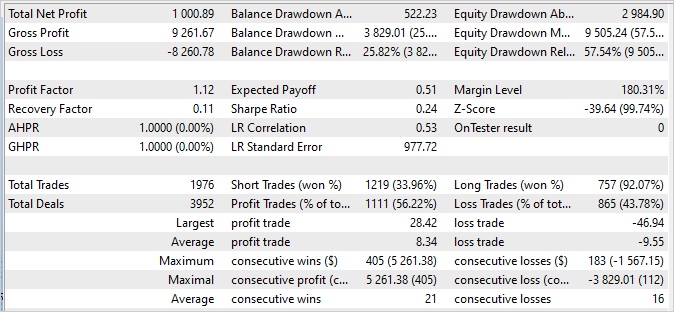
350668273_1631799953971007_1316803797828649367_n.png (1115×666) (fbcdn.net)After some successful training, I was able to achieve a 99% win rate. However, it only sold trades. no buy trades
Here's a screenshot:
350733414_605596475011106_6366687350579423076_n.png (1909×682) (fbcdn.net)
Dmitriy,
I am following your articles to learn as much as possible as your knowledge and expertise is way beyond me. After reading the article, it occurred to me that while the final model presented is excellent at identifying short trades and totally unsuccessful at identifying long trades, it could be part of a two tier trading solution. A long trade model is needed to complement the short trades. Do you think the long model could be developed by reversing some of the assumptions or is a wholly new model required, such as toe Go Explore in article #39?
Cheers on your current efforts and support for your future endeavors