The case for using Hospital-Performance Data with Perceptrons, this Q4, in weighing SPDR XLV's next Performance

Introduction

SPDR’S XLV ETF is the pool of healthcare related stocks listed on the S&P 500 that can be bought by investors who want specific exposure to the healthcare sector. It is one of 11 sector ETFs retailed under SPDR by State Street Global Advisors. With its inception on December of 1998, it currently holds a little over U$36 billion in assets under management.

This article aims to look at a variety of datasets related to the ETF XLV, that could be key in driving momentum and or setting direction for the ETF. And the approach to be adopted here will be to select one of these data sets as a feed to a multi-layer perceptron. Perceptron’s can work with any data set in making a forecast so we attempt to answer the question which of the available datasets, pertinent to XLV, is better suited in light of the recent quarter performance & news to make the projection for the next quarter’s momentum. This is a very critical step for which am sure traders who use perceptrons have to consider from time to time. Our methodology will primarily dwell on using feature importance for data analysis to make this selection.

In the recent trailing quarter for XLV we have witnessed some selling off which markets are attributing to the waning off of the covid-19 pandemic, whose vaccines were a key driver for performance 2021-2022. But also, at a macro level a hawkish Fed is setting up bearish undertones in the market which are putting a lot of selling pressure on many ETFs right across the sectors. Medical Breakthroughs, Clinical trial results, FDA Drug approvals, and FDA Safety alerts, etc. have all played a part in the performance of XLV this past quarter which is why it would be helpful to start by listing the possible datasets we should consider for our model.

Data Sources

The data sources to be considered are from US government websites, US government agency websites, and some 3^rd party researchers who may have data that is not readily available yet in the public domain but is pertinent to XLV performance.

Data sources are very important because the quality of your data set is in large part defined by your source which is why it is a good idea to get your data from established websites like the FDA, or Clinical Trials when doing analysis. In our case, for this article we are leaning away from government policy dependent data and more towards market/ research data that’s why we have not referred to the FDA website. Kaggle though not in the same league as the FDA, or Clinical Trials is growing in use and could soon be established as one of the bell-weathers.

The timeframe across these datasets is not consistent as it is largely determined by the data source. The time frames are daily, annual, and weekly.

Available Data Sets for XLV

So, the broad picture in XLV seems to be the waning impact of government vaccine mandates which could mean it is not the time to rely on government derived data sets like FDA safety alerts, but rather a time to consider more what is happening ‘on the ground’ with different data sets like Clinical trial results. This is a simplistic approach but for this article it will suffice in guiding our data set selection approach. The number of data sets, within this sub-category, that are more market than government oriented and are applicable to XLV is arguably a lot however for our purposes we will look at a short abridged list. 

The data sets for XLV performance, historical volatility, and trade volume all come under 5 headers of which 4 (excluding the date) will be used in the analysis. A typical representation of this is in the image below:

 

Date	Open change	High change	Low change	Close change	Classifier or Dependent Variable

 

So, these are the headers to the attached csv files. ‘Change’ stands for the percentage difference from the previous price. What is meant by ‘price’ is clarified below for each of the 3 data sets.

XLV historical performance:

XLV’s historical price changes as a percentage can easily be computed from closing daily prices that available online from a host of websites. If we are to use R to export this as a csv for use with MetaTrader, then we would simply have to follow these R coding steps.

Install the quantmod package.

install.packages(“quantmod”)

Use its library.

library(quantmod) 

Import last 2 quarters of XLV data into R

getSymbols("XLV",src="yahoo",from="2023-05-01", to="2023-11-01") 

Export the data as a csv.

write.zoo(XLV, "xlv.csv", sep = ",")

From the exported csv values, we can easily compute percentage changes in close price and generate a daily time series from this for our model. Past performance can auto-correlate with future performance in certain markets, so this data set can be handy in those situations. Because we need a rich data set with more than one feature/ column, our data set can capture the percentage changes for the open high low and close prices. These multiple columns will allow for a fair comparison against other data sets that have multiple columns by default.

XLV historical volatility:

Historical volatility is a common indicator, even though not renown as its illustrious cousin implied volatility, for our purposes it is one we can generate easily from the csv file above and use as an input data set. The formula can simply be the standard deviation of the percentage changes we computed above. These changes were from day to day. If we measured all daily changes off of an absolute datum, say the beginning of a week then the standard deviation of these changes would also be the quarterly historical volatility. It is argued that in markets that tend to trend long over the long haul such as the S&P 500 or this constituent ETF, high volatility portends a bearish outlook while low volatility could indicate the opposite. This feature could make this data set relevant in forecasting for our model.

XLV historical trade volume:

Contract trade volume which is also publicly available, can be engaged as a data set and if we use the csv export from R above we can easily create a time series of these values on the daily time frame. Contract volume could serve as an indicator to future performance in certain situations, such as when confirmation is needed after a price break out, among other use cases that’s why we’ve included it as a potential data set for our model. It will also be used with four columns despite being a single column of daily contracts. How we achieve this will be by assigning a volume weight (not VWAP) to each of the open, high, low, and close performance values by multiplying them with the current volume of the day then dividing the product by the cumulative contract volume for the trailing week.

Health insurance claims:

As we start to consider the ‘fundamentals’ of the healthcare sector the data sets available for this analysis becomes more disparate. In the US, States mandate insurance companies to file data on their insurance claims. To try to aggregate this information state by state would be a pitiful exercise which is why the National Association of Insurance Commissioners’ website is a godsend. There is a lot of data not just by state but also relating to insurance premiums and claims and unfortunately it is too aggregated, with the figures being reported annually. This means if we are to consider this data set then the projections made by our model would also have to be looking forward by a year at least. On the plus side though, data sets here have a lot of varying columns (features), which is unlike the three data set time series of performance, volatility, and volume which mentioned above that have standard four features each (for OHLC). The annual timeframe data set to be considered is available here on page 5 (10yr summary) of the pdf file and the 3 features of each data row are: time (or year), direct premiums earned, and direct claims incurred. Increased number of features may make this data set more accurate in forecasts. The header row for this data set will be as shown below. This information is not part of the csv file for efficiency in processing the data.

Date	Premium Earned	Claims Incurred	Dependent Variable

 

Pharmaceutical sales:

Kaggle is a growing platform for publicly available data sets that can be used in machine learning models and perhaps it would be good to have a look for something on sales in pharmaceuticals. Unlike insurance claims that include both cover for medication and healthcare provider compensation, pharmaceutical sales focus on monies paid for medicine. This granularity could be insightful in providing guidance for XLV, with a presumed positive auto-correlation, which is why we have included it in our list. A number of candidate data sets can be viewed from the website here, and as mentioned above they are not as structured as the price data time series we considered for the first 3 data sets. Our best option from what is available as of writing this article is this data set which unfortunately covers 2021 only and nothing since. This means our model will only train on data within 2021 if this data set is chosen. It also has more than 5 features which poses more choice on what to include and omit when using the model. (Update: Macro sales data with 2 columns was used instead, it runs from 2010 – 2020, on an annual time frame) The column names to this data set are laid out as below. This is not indicated on the attached csv files.

Date	US Sales (U$ Bn)	International Sales (U$ Bn)	Dependent Variable

 

Hospital performance metrics:

The metrics of a hospital’s performance can also be taken to be accretive to XLV’s future performance as simple logic would imply if most hospitals are doing well, so will the XLV price in the long run. Picking a representative data set on this is even more derisive than our previous two since it is more subjective given the need for human patient feedback. The data set we’ll consider thus cover healthcare patient satisfaction and it is available here also at Kaggle. Once again there could be more up to date data sets as this one does not go beyond 2020, however it is large enough to allow training and if and when more current data set(s) are acquired then forecasting with the model can be done. The number of features in this data set are also a lot and they are not regressive because they are text. (Update: Used a simpler data set, sourced from Google’s Bard consisting of hospital stay and number of available beds that ran from a decade back to present day)  The hospital performance header is as shown below:

Date	Average Hospital Stay (Days)	Total Hospital Beds	Dependent Variable

Disease prevalence data:

Data on this subject can also relate inversely to XLV’s performance where in the short run if for instance there is an onset of a pandemic it can be understood that healthcare companies are not yet ready to address the spreading illness and are missing out on revenue growth, with high capex for research. However, in the mid-long run the opposite could also be true where once vaccines/ drugs are developed for the outbreak, then the healthcare companies will have a boon. Again, a lot of data sets to choose from and what complicates matters here is a lot of research is ongoing in correctly identifying the various diseases take for instance during the covid-19 outbreak there was a near fall off in the number of deaths attributed to common cold yet this number in prior years had been high. So, it’s with this hindsight that we’ll use weekly counts of deaths and not statistics on any particular disease. It can be understood that the deaths count would tend to positively correlate with disease prevalence. We use Kaggle again and source our up to date sample from here. Interestingly the features (data columns) of this data set are the various diseases attributed to the mortality, so we could select some of these columns, not all, as part of the data set. The disease prevalence data set has the most features and its header is as indicated below:

Date	All Cause	Natural Cause	Influenza & Pneumonia	Heart Disease	Covid

 

 

Clinical trials:

Our final data set is often mentioned as key when looking at healthcare but actually using it with a broad index like XLV, or even a particular stock, can be problematic because clinical trials are often specific to a particular drug of a specific company. Simply tying them down to a company will not help matters as far as building a time series is concerned because the drug pipeline of each company is not necessarily regular, sometimes they could be doing research in other times they may not so the data set is bound to have a few gaps. The question of which drug to focus on those under study is rather pertinent since XLV is a holding of several healthcare related companies. That’s why for this article we will stick to covid-19 related drugs since they tend to concern a wide variety of healthcare companies than other alternatives. Our data set is sourced from clinical trials website here and like most of the data sets referred to above it is attached at the end of the article. This data set has the following header representation:

Date	Phase 1 trials	Phase 2 trials	Phase 3 trials

Feature Importance and Data Selection

Feature importance at its core weighs the significance of the various columns in a data set by assigning them values typically less than one that all add up to one across the columns. This relative weighting of the columns can be interpreted to speak to the relevance of the data set in determining their classifier or forecast value. There are several methods that can be used in determining these weightings, the one we will focus on is the Gini coefficient as implemented by decision forests. Our code listing in mql5 for achieving this is shared below:

//+------------------------------------------------------------------+
//|                                                                  |
//+------------------------------------------------------------------+
class Cgini
{
protected:

public:
      CDForest f;
      CDecisionForest m;
      CDecisionForestBuilder b;
      
      CDFReport r;
      
      CMatrixDouble xy;
      
      bool Get(string FileName);
      void Set(string FileName);
      
      int tracks,features;
      
   Cgini();
   ~Cgini();
};

//+------------------------------------------------------------------+
//|                                                                  |
//+------------------------------------------------------------------+
Cgini::Cgini()
{
   tracks=0;
   features=0;
}
//+------------------------------------------------------------------+
//|                                                                  |
//+------------------------------------------------------------------+
bool Cgini::Get(string FileName)
{
   string _array_rows[],_array_columns[];
   int _line = 0, _max_columns=INT_MIN;
   //
   ResetLastError();
   int _handle=FileOpen(FileName+"_w.csv",FILE_SHARE_READ|FILE_CSV|FILE_COMMON,'\n');
   
   if(_handle!=INVALID_HANDLE)
   {
      _line = 0; _max_columns=INT_MIN;
      //
      while(!FileIsEnding(_handle))
      {
         string _file  = FileReadString(_handle);
         
         _max_columns  = fmax(_max_columns,StringSplit(_file,',',_array_columns));
         //
         xy.Resize(_line+1,_max_columns-1);
         //
         for(int ii=1;ii<_max_columns;ii++)
         {
            xy.Set(_line,ii-1,StringToDouble(_array_columns[ii]));
         }
         _line++;
      }
      //
      FileClose(_handle);
   }
   else
   {
      printf(__FUNCSIG__+" failed to create read build handle for: "+FileName+", err: "+IntegerToString(GetLastError()));
      FileClose(_handle);
      return(false);
   }
         
   return(true);
}
//+------------------------------------------------------------------+
//|                                                                  |
//+------------------------------------------------------------------+
void Cgini::Set(string FileName)
{
      f.DFBuilderCreate(b);
      f.DFBuilderSetDataset(b,xy,xy.Rows(),xy.Cols()-1,1);
      f.DFBuilderSetImportanceTrnGini(b);
      f.DFBuilderSetSubsampleRatio(b,1.0);
      f.DFBuilderBuildRandomForest(b,50,m,r);
      double _i[];r.m_varimportances.ToArray(_i);
      double _dev=MathStandardDeviation(_i);
      //
      printf(__FUNCSIG__+" "+FileName+" dispersion is: "+DoubleToString(_dev));
}
//+------------------------------------------------------------------+
//|                                                                  |
//+------------------------------------------------------------------+
Cgini::~Cgini()
{
}
//+------------------------------------------------------------------+

The Gini coefficient used in measuring the weight of each data column does so via AlgLib’s decision forest class. The report’s output parameter ‘m_varimportances’ which is computed provided we call the ‘Set Importance’ function, will be an array with the weights of each data column in the data set. So, its array size matches the number of columns or features in the data set.

So, to compute the feature importance of our highlighted data sets above, all data will be retrieved from a csv file that was created when the data was exported. For XLV performance if we run the script with our feature importance code listed above, we get the following results:

2023.11.09 17:13:37.856 xlv_1 (EURJPY.ln,W1)    void Cgini::Set(string) performance_1 dispersion is: 0.06129706
2023.11.09 17:13:46.391 xlv_1 (EURJPY.ln,W1)    void Cgini::Set(string) performance_1 dispersion is: 0.09403280

For historical volatility we have:

2023.11.09 17:21:02.418 xlv_1 (EURJPY.ln,W1)    void Cgini::Set(string) volatility_1 dispersion is: 0.08262673
2023.11.09 17:21:21.758 xlv_1 (EURJPY.ln,W1)    void Cgini::Set(string) volatility_1 dispersion is: 0.04689318

Likewise, for contract volume we have:

2023.11.09 17:20:23.362 xlv_1 (EURJPY.ln,W1)    void Cgini::Set(string) volume_1 dispersion is: 0.04950861
2023.11.09 17:20:32.689 xlv_1 (EURJPY.ln,W1)    void Cgini::Set(string) volume_1 dispersion is: 0.06853639

And for insurance claims we get:

2023.11.09 17:19:31.934 xlv_1 (EURJPY.ln,W1)    void Cgini::Set(string) insurance_claims_1 dispersion is: 0.46951890
2023.11.09 17:19:44.769 xlv_1 (EURJPY.ln,W1)    void Cgini::Set(string) insurance_claims_1 dispersion is: 0.50958829

With pharmaceutical sales we have:

2023.11.09 17:18:15.009 xlv_1 (EURJPY.ln,W1)    void Cgini::Set(string) pharmaceutical-sales_1 dispersion is: 0.46322455
2023.11.09 17:18:39.732 xlv_1 (EURJPY.ln,W1)    void Cgini::Set(string) pharmaceutical-sales_1 dispersion is: 0.52973056

For hospital metrics we get:

2023.11.09 17:16:31.272 xlv_1 (EURJPY.ln,W1)    void Cgini::Set(string) hospital_performance_1 dispersion is: 0.33683033
2023.11.09 17:16:56.274 xlv_1 (EURJPY.ln,W1)    void Cgini::Set(string) hospital_performance_1 dispersion is: 0.30905792

With disease prevalence we get:

2023.11.09 17:15:33.549 xlv_1 (EURJPY.ln,W1)    void Cgini::Set(string) disease_prevalance_1 dispersion is: 0.01393427
2023.11.09 17:15:50.536 xlv_1 (EURJPY.ln,W1)    void Cgini::Set(string) disease_prevalance_1 dispersion is: 0.01369283

And finally, for clinical trials we get:

2023.11.09 17:14:15.846 xlv_1 (EURJPY.ln,W1)    void Cgini::Set(string) clinical_trials_1 dispersion is: 0.29143323
2023.11.09 17:14:46.849 xlv_1 (EURJPY.ln,W1)    void Cgini::Set(string) clinical_trials_1 dispersion is: 0.28867513

From our runs above, the data set with the least dispersion in weights is death prevalence data set. Not far from it are the performance, contract volume and volatility data sets. The datasets with considerable dispersion, and arguably importance though, are insurance claims, pharmaceutical sales, hospital performance, and clinical trials. Because the importance scores are got via random forest, the script needs to be run twice to confirm the reading and as can be shown above the two runs for any data set do not give identical readings but the figures are in the same ball park. So the winning data set, by feature importance, would be insurance claims data.

Multi-Layer Perceptron Model

Our model choice for using the selected data set is a multi-layer perceptron. It is relatively more widely used than other options and AlgLib provides an out of box implementation that can save a lot on the need for customization. There are not a lot of MetaTrader Brokers that offer trading ETF CFDs, and of the few that do, I could not find one with the XLV ETF specifically. The broker that was sourced and had ETFs but no XLV did have stocks, of which United Health, which is currently the largest holding in XLV, was available. So, to test our data sets above we’ll use this equity stock as a proxy and we’ll run tests across the data set period while concurrently doing training on history periods before the test run period. To illustrate if our training points are 5 we will begin running forward tests at index 6 because the first 5 data values will be used in training. On shifting to index 7, we again train our perceptron on the 5 data points prior to 7 which will be from 6 to 2, and so forth. So, with this setup we are constantly training with recent history and are using those weights to make a forward pass feed with the current variables. Our data sets have various numbers of independent variables and they also come in different ‘timeframes’. This means our testing expert advisor needs to be able to handle all these variables on the fly and still execute. Also, our tested symbol, and probably the ETF XLV if it would have been available, can only be traded within a short hour window so our expert advisor should also make sufficient provision for this to avoid ‘market closed’ errors. I think it always better to test entry signal ideas within expert signal classes that are can be assembled in the MQL5 wizard, in this instance though given the use of very large time frames such as quarterly, some are even annual, it is prudent to do a custom implementation.

Initializing the MLP and setting up the sizes of the input and output layers is straight forward with this class and AlgLib references can be used by anyone who may need some guidance.

For our purposes the listing is part of the expert initialization as follows:

//+------------------------------------------------------------------+
//| Expert initialization function                                   |
//+------------------------------------------------------------------+
int OnInit()
  {
   ...

   //
   if(_g.Get(__data_set))
   {
      _g.Set(__data_set);
      
      if(__training_points>=_g.xy.Rows()-1)
      {
         printf(__FUNCSIG__+" too many training points given sample size. ");
         return(INIT_PARAMETERS_INCORRECT);
      }
      
      int _inputs=_g.xy.Cols()-1;
      int _outputs=1;
      
      ...
         
      _xy.Resize(__training_points,_inputs+_outputs);
      
      if(!ReadWeights())
      {
         _mlp.m_weights.Fill(1.0);
      }
      
      //
      
      if(__hidden==0)
      {
         _base.MLPCreate0(_inputs,_outputs,_mlp);
      }
      else if(__hidden==1)
      {
         if(__hidden_1_size<=_inputs)
         {
            printf(__FUNCSIG__+" hidden 1 size should exceed inputs. ");
            return(INIT_PARAMETERS_INCORRECT);
         }
         _base.MLPCreate1(_inputs,__hidden_1_size,_outputs,_mlp);
      }
      else if(__hidden==2)
      {
         if(__hidden_1_size<=_inputs)
         {
            printf(__FUNCSIG__+" hidden 1 size should exceed inputs. ");
            return(INIT_PARAMETERS_INCORRECT);
         }
         if(__hidden_2_size<=_outputs)
         {
            printf(__FUNCSIG__+" hidden 2 size should exceed outputs. ");
            return(INIT_PARAMETERS_INCORRECT);
         }
         _base.MLPCreate2(_inputs,__hidden_1_size,__hidden_2_size,_outputs,_mlp);
      }
      else if(__hidden>2||__hidden<0)
      {
         printf(__FUNCSIG__+" invalid number of hidden layers should be 0, 1, or 2. ");
         return(INIT_PARAMETERS_INCORRECT);
      }
      
      _train.MLPCreateTrainer(_inputs,_outputs,_trainer);
      
      __IN_TRAINING=false;
   }
   else
   {
      printf(__FUNCSIG__+" missing csv file... ");
      return(INIT_PARAMETERS_INCORRECT);
   }
   
   
...
   
//---
   return(INIT_SUCCEEDED);
  }

 

What could be noteworthy here is determining the number of hidden layers for this MLP. How many should they be? And what size should each be? Our testing will use 5 points in the first hidden layer and 3 in the second hidden layer. These can be adjusted by the reader but in order to minimize biases at this very preliminary testing stage everything will be uniform for all data sets. The perceptron model used here does not allow more than 2 hidden layers out of the box. There are work arounds this but they are not the subject for this article so we will work within this limitation.

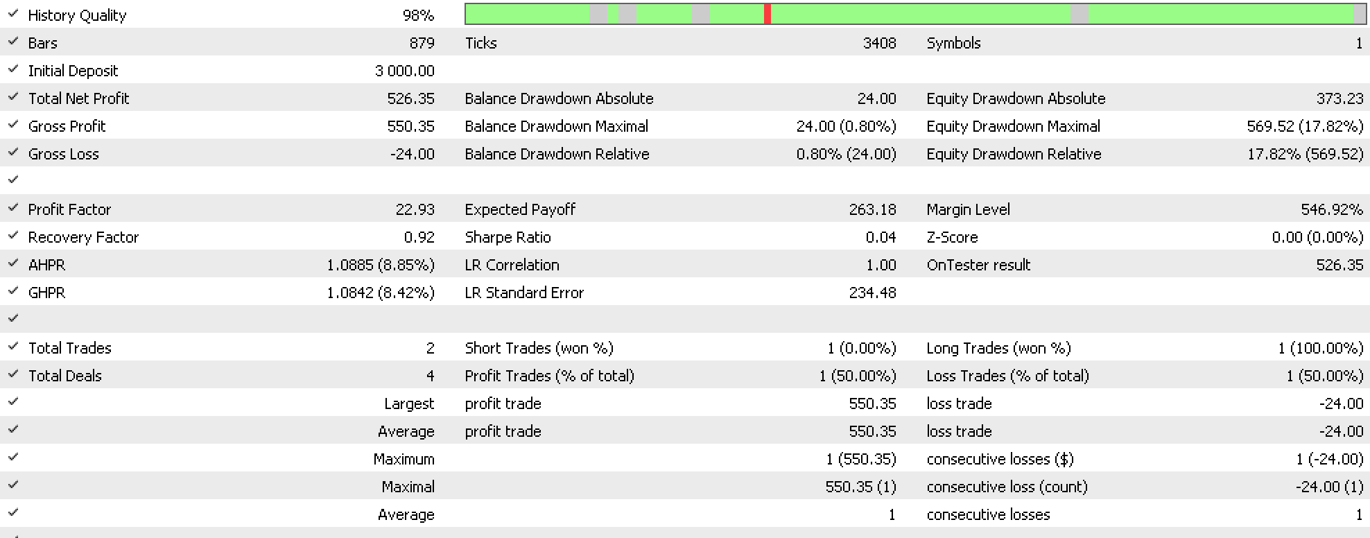
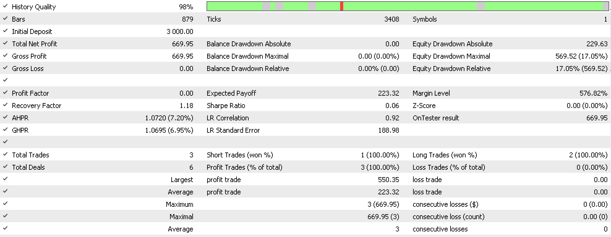
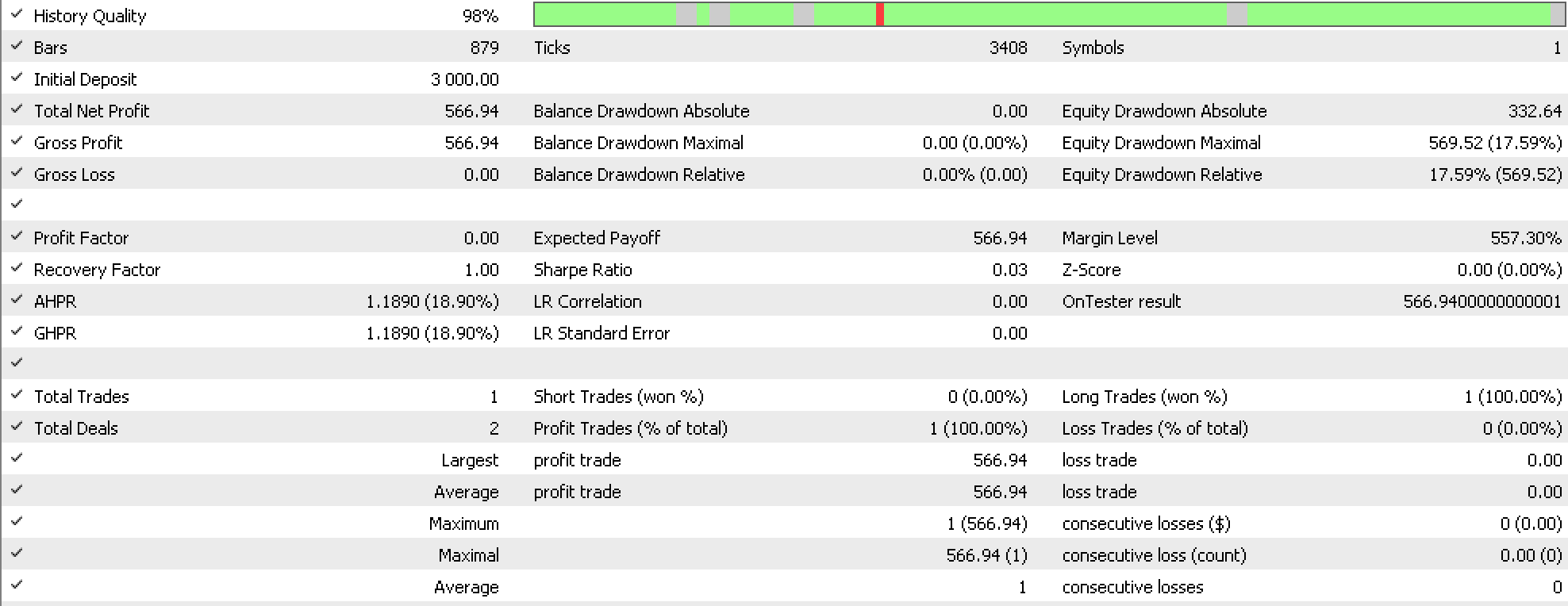
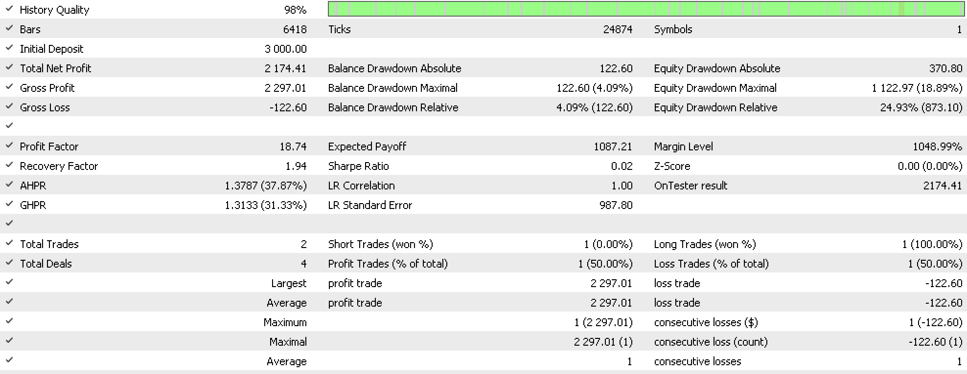
Also in the test runs for the data sets our custom expert advisor opens positions and holds them until there is a signal reversal. Price targets, and stop losses or trailing stops are not employed. We will perform test runs on the 6 data sets that have time frames smaller than annual which are performance, volume, volatility, hospital-performance, disease-prevalence, and clinical trials. The input settings and report-results over the data set period (minus training size) are shown below:

 

Performance:

 

 

 

Volatility:

 

Volume:

 

Disease Prevalence:

 

Hospital Performance:

 

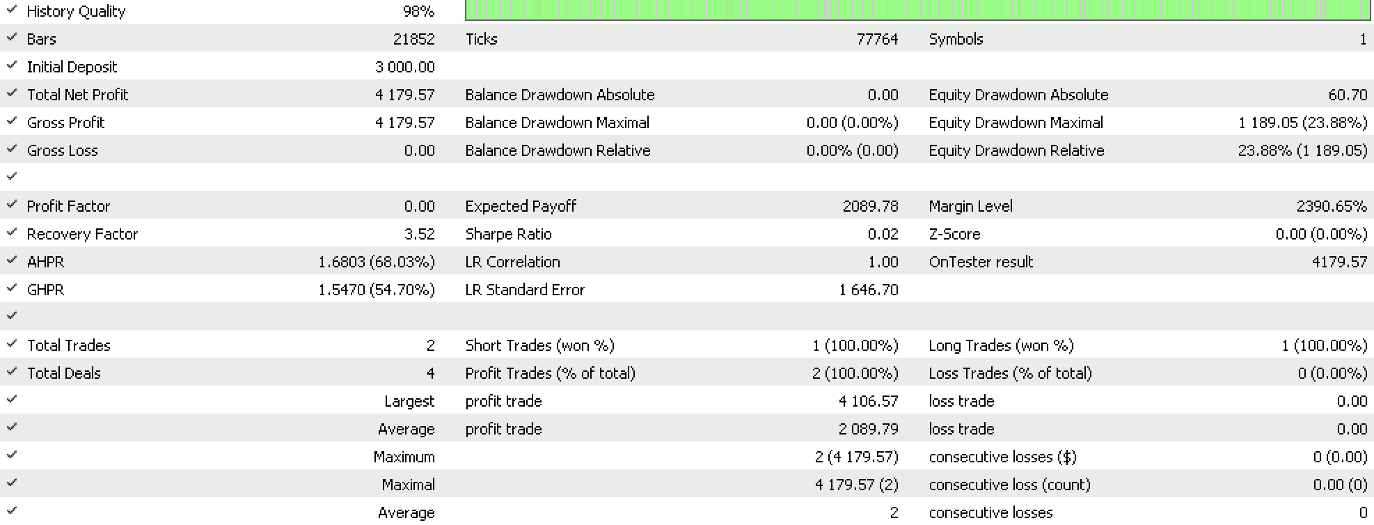
Clinical Trials:

 

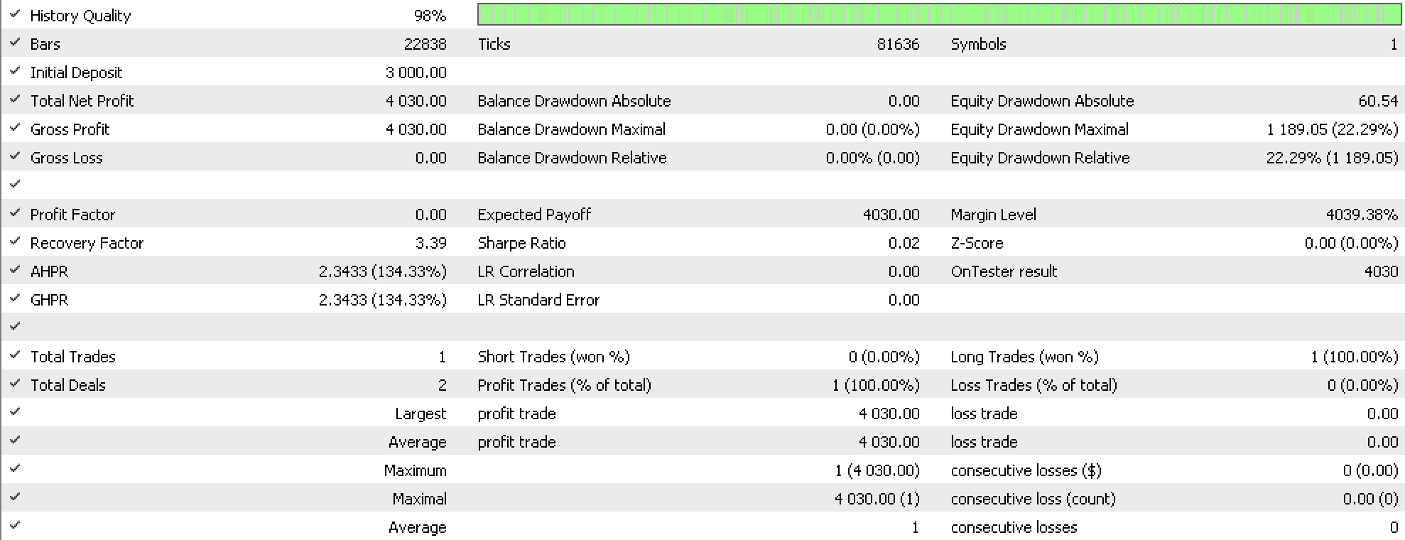
All data sets do not place a lot of trades so the argument for more testing over longer periods is valid. Hospital performance data set which had a decent feature importance number comes out on top. Insurance Claims and pharmaceutical sales could even do better but these have not been tested given the large timeframe and small test sample, but this is always open to exploration.

Also noteworthy is that the network weights are saved at the end of a test run if a better test result (as per the test criterion) has been registered in the run. These weights can be re-used in different runs and testing to minimize on training efforts.

Conclusion

So, to recap the key point covered here is feature importance, as evaluated using the Gini-coefficient can be instrumental in sifting through the multitude of data sets one is faced with when training a model. Our choice of model for this article was the Multi-Layer Perceptron and AlgLib’s code library allows easy implementation in MetaTrader’s IDE.  

Data sets that span large time frames and avoid the day to day noise tend to have higher importance scores and are therefore worth considering for use in models, with the winner from the testing done on data sets presented in this article being hospital performance data.

Using this or better scoring data sets will require more diligence with MLPs by for instance by establishing the number of hidden layers to use and the size of each of these layers, aspects which have not been properly addressed here but the reader can pursue.