
Data Science and Machine Learning — Neural Network (Part 02): Feed forward NN Architectures Design
“I’m not suggesting that neural networks are easy. You need to be an expert to make these things work. But that expertise serves you across a broader spectrum of applications. In a sense, all of the effort that previously went into feature design now goes into architecture design and loss function design and optimization scheme design. The manual labor has been raised to a higher level of abstraction.”
--Stefano Soatto
Introduction
In the prior article, we discussed the basics of a neural network and build a very basic and static MLP, but we know in real-life applications we are not going to need a simple 2 inputs and 2 hidden layers nodes in the network to the output, something we built last time.
Sometimes a network that works best for your problem might be the one with 10 nodes in the inputs layer, 13 nodes/neurons in the hidden layer and something like four or something in the output layer not to mention you are going to have to tune the number of hidden layers in the entire network.
My point is that we need something dynamic. A dynamic code that we can change the parameters and optimize without breaking the program. If you use python-keras library to build a neural network you will have to do less work of configuring and compiling even complex architectures, that is something that I want us to be able to achieve in MQL5.
Just like I did on the Linear regression part 3 which is one among the must-read in this article series, I introduced the matrix/vector form of models to be able to have flexible models with an unlimited number of inputs.
Matrices Comes to the Rescue
We all know that hard-coding models fall flat when it comes to wanting to optimize for the new parameters, the whole procedure is time-consuming, causes headaches, pain in the back etc. (It's not worth it)
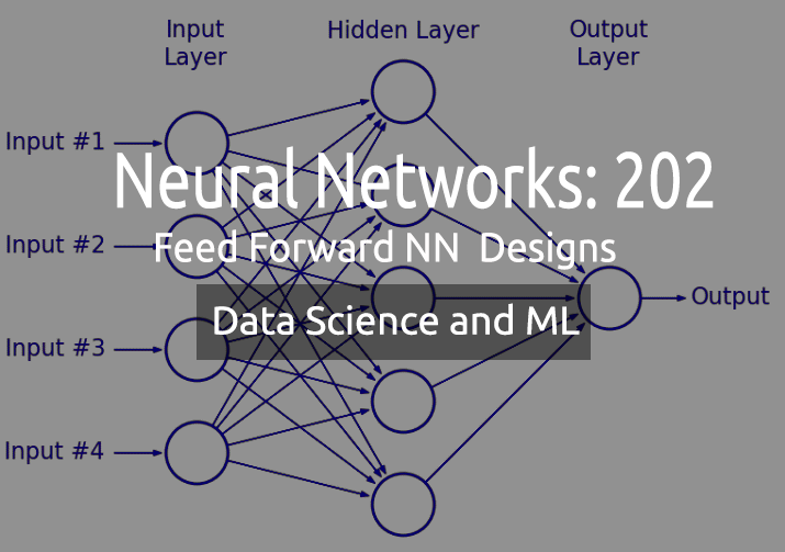
If we take a closer look at the operations behind a neural network you'll notice that each input gets multiplied to the weight assigned to it then their output gets added to the bias. This can be handled well by the matrix operations.
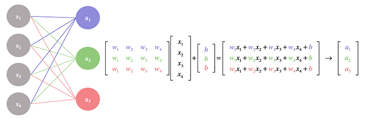
Basically, we find the dot product of the Input and the weight matrix then we finally add it to the bias.
For the sake of building a flexible neural network, I am going to try an odd architecture of 2 nodes in the input layer, 4 in the first hidden layer, 6 in the second hidden layer and 1 in the third hidden layer, and finally one node in the output layer.
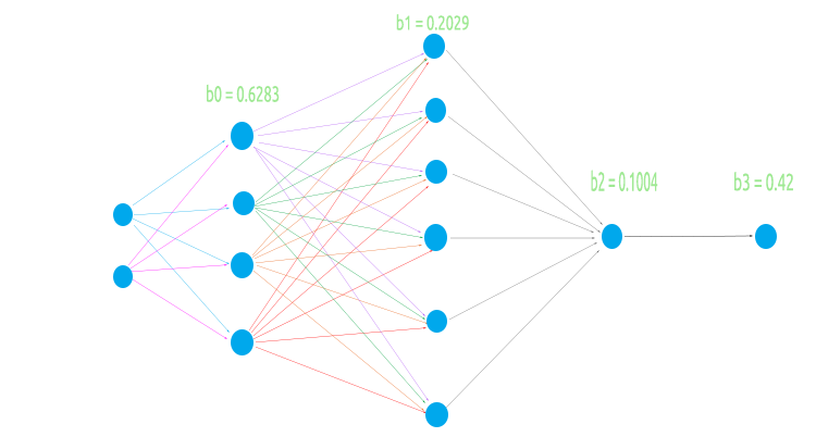
This is for the sake of testing if our matrix logic will go smoothly in all case scenarios
- When the previous (input) layer has few numbers nodes that the next layer (output layer)
- When the previous (input) layer has a lot of nodes that the next layer
- When there is an equal number of nodes in the input layer and the next layer (output) layer
Before we code for the matrix operations and compute the values, let's do the basic stuff that is going to make the entire operation possible.
Generating the random weights and bias values.
    //Generate random bias
    for(int i=0; i<m_hiddenLayers; i++)         bias[i] = MathRandom(0,1);

    //generate weights
    int sum_weights=0, L_inputs=inputs;
    double L_weights[];

    for (int i=0; i<m_hiddenLayers; i++)
      {
         sum_weights += L_inputs * m_hiddenLayerNodes[i];
         ArrayResize(Weights,sum_weights);
         L_inputs = m_hiddenLayerNodes[i];
      }

    for (int j=0; j<sum_weights; j++) Weights[j] = MathRandom(0,1);
We saw this operation in the previous part but, one thing to notice is that these values of the weight and bias are supposed to be generated once to be used in the cycle of epochs.
What is an Epoch?
An epoch is a complete pass of all the data in the neural network, in a feedforward is an entire forward pass of all the inputs, in a backpropagation is an entire forward and backward pass. In simple words is when a neural network has seen all the data.
Unlike in the MLP we've seen in the previous article this time we are coming with an implementation that takes into consideration the Activation Function in the output layer something those who use keras probably familiar with, basically we can have different activation function in the hidden layer and the one that leads to the output in the output layer.
CNeuralNets(fx HActivationFx,fx OActivationFx,int &NodesHL[],int outputs=NULL, bool SoftMax=false);
Pay attention to the Inputs HActivationFx is for the Activation function in the hidden layers, OActivationFx is for the Activation function in the output layer, NodesHL[] is for the number of Nodes in the hidden layer. If that array has let's say 3 elements, it means that you will have 3 hidden layers and the number of nodes in those layers will be determined by the elements present inside the array, see the below code.
int hlnodes[3] = {4,6,1};
int outputs = 1;

neuralnet = new CNeuralNets(SIGMOID,RELU,hlnodes,outputs);
This is the Architecture on the image we just seen above. The outputs argument is optional, if you leave it to NULL the following configuration will be applied to the outputs layer:
if (m_outputLayers == NULL)
{
  if (A_fx == RELU)     m_outputLayers = 1;
  else                  m_outputLayers = ArraySize(MLPInputs);
}
If you chose the RELU as an Activation Function in the hidden layer, the output layer will have one node, otherwise the number of outputs in the final layer will be equal to the number of the inputs in the first layer. Chances are high you are using a classification neural network if you are using other activation function than RELU in the hidden layer so the default output layer will be equal to the number of columns. This is unreliable though the outputs must be the number of targeted features from your dataset if you are trying to solve a classification problem, I will find a way to change this in the further updates, right now you have to choose manually the number of output neurons.
Now, let's call the complete MLP Function and see the output then I will explain what has been done to make the operations possible.
LI      0       10:10:29.995    NNTestScript (#NQ100,H1)        CNeural Nets Initialized activation = SIGMOID UseSoftMax = No
IF      0       10:10:29.995    NNTestScript (#NQ100,H1)        biases
EI      0       10:10:29.995    NNTestScript (#NQ100,H1)        0.6283 0.2029 0.1004
IQ      0       10:10:29.995    NNTestScript (#NQ100,H1)        Hidden Layer 1 | Nodes 4 | Bias 0.6283
NS      0       10:10:29.995    NNTestScript (#NQ100,H1)        Inputs 2 Weights 8
JD      0       10:10:29.995    NNTestScript (#NQ100,H1)        4.00000 6.00000
FL      0       10:10:29.995    NNTestScript (#NQ100,H1)        0.954 0.026 0.599 0.952 0.864 0.161 0.818 0.765
EJ      0       10:10:29.995    NNTestScript (#NQ100,H1)        Arr size A 2
EM      0       10:10:29.995    NNTestScript (#NQ100,H1)        AxBMatrix[0] = 3.81519 X A[0] = 4.000 B[0] = 0.954
NI      0       10:10:29.995    NNTestScript (#NQ100,H1)        AxBMatrix[0] = 9.00110 X A[1] = 6.000 B[4] = 0.864
IE      0       10:10:29.995    NNTestScript (#NQ100,H1)        AxBMatrix[1] = 0.10486 X A[0] = 4.000 B[1] = 0.026
DQ      0       10:10:29.995    NNTestScript (#NQ100,H1)        AxBMatrix[1] = 1.06927 X A[1] = 6.000 B[5] = 0.161
MM      0       10:10:29.995    NNTestScript (#NQ100,H1)        AxBMatrix[2] = 2.39417 X A[0] = 4.000 B[2] = 0.599
JI      0       10:10:29.995    NNTestScript (#NQ100,H1)        AxBMatrix[2] = 7.29974 X A[1] = 6.000 B[6] = 0.818
GE      0       10:10:29.995    NNTestScript (#NQ100,H1)        AxBMatrix[3] = 3.80725 X A[0] = 4.000 B[3] = 0.952
KQ      0       10:10:29.995    NNTestScript (#NQ100,H1)        AxBMatrix[3] = 8.39569 X A[1] = 6.000 B[7] = 0.765
DL      0       10:10:29.995    NNTestScript (#NQ100,H1)        before rows 1 cols 4
GI      0       10:10:29.995    NNTestScript (#NQ100,H1)        IxWMatrix
QM      0       10:10:29.995    NNTestScript (#NQ100,H1)        Matrix
CH      0       10:10:29.995    NNTestScript (#NQ100,H1)        [
HK      0       10:10:29.995    NNTestScript (#NQ100,H1)        9.00110 1.06927 7.29974 8.39569
OO      0       10:10:29.995    NNTestScript (#NQ100,H1)        ]
CH      0       10:10:29.995    NNTestScript (#NQ100,H1)        rows = 1 cols = 4

<<<<<<<<<<<<<<<<<<<<<<<<<<<<<<<<<< End of the first Hidden Layer >>>>>>>>>>>>>>>>>>>>>>>>>>>>>>>>>>>>>>>>>>>>>>>>>>>>>>>>>>>>>>>>

NS      0       10:10:29.995    NNTestScript (#NQ100,H1)        Hidden Layer 2 | Nodes 6 | Bias 0.2029
HF      0       10:10:29.995    NNTestScript (#NQ100,H1)        Inputs 4 Weights 24
LR      0       10:10:29.995    NNTestScript (#NQ100,H1)        0.99993 0.84522 0.99964 0.99988
EL      0       10:10:29.996    NNTestScript (#NQ100,H1)        0.002 0.061 0.056 0.600 0.737 0.454 0.113 0.622 0.387 0.456 0.938 0.587 0.379 0.207 0.356 0.784 0.046 0.597 0.511 0.838 0.848 0.748 0.047 0.282
FF      0       10:10:29.996    NNTestScript (#NQ100,H1)        Arr size A 4
EI      0       10:10:29.996    NNTestScript (#NQ100,H1)        AxBMatrix[0] = 0.00168 X A[0] = 1.000 B[0] = 0.002
QE      0       10:10:29.996    NNTestScript (#NQ100,H1)        AxBMatrix[0] = 0.09745 X A[1] = 0.845 B[6] = 0.113
MR      0       10:10:29.996    NNTestScript (#NQ100,H1)        AxBMatrix[0] = 0.47622 X A[2] = 1.000 B[12] = 0.379
NN      0       10:10:29.996    NNTestScript (#NQ100,H1)        AxBMatrix[0] = 0.98699 X A[3] = 1.000 B[18] = 0.511
MI      0       10:10:29.996    NNTestScript (#NQ100,H1)        AxBMatrix[1] = 0.06109 X A[0] = 1.000 B[1] = 0.061
ME      0       10:10:29.996    NNTestScript (#NQ100,H1)        AxBMatrix[1] = 0.58690 X A[1] = 0.845 B[7] = 0.622
PR      0       10:10:29.996    NNTestScript (#NQ100,H1)        AxBMatrix[1] = 0.79347 X A[2] = 1.000 B[13] = 0.207
KN      0       10:10:29.996    NNTestScript (#NQ100,H1)        AxBMatrix[1] = 1.63147 X A[3] = 1.000 B[19] = 0.838
GI      0       10:10:29.996    NNTestScript (#NQ100,H1)        AxBMatrix[2] = 0.05603 X A[0] = 1.000 B[2] = 0.056
GE      0       10:10:29.996    NNTestScript (#NQ100,H1)        AxBMatrix[2] = 0.38353 X A[1] = 0.845 B[8] = 0.387
GS      0       10:10:29.996    NNTestScript (#NQ100,H1)        AxBMatrix[2] = 0.73961 X A[2] = 1.000 B[14] = 0.356
CO      0       10:10:29.996    NNTestScript (#NQ100,H1)        AxBMatrix[2] = 1.58725 X A[3] = 1.000 B[20] = 0.848
KH      0       10:10:29.996    NNTestScript (#NQ100,H1)        AxBMatrix[3] = 0.59988 X A[0] = 1.000 B[3] = 0.600
OD      0       10:10:29.996    NNTestScript (#NQ100,H1)        AxBMatrix[3] = 0.98514 X A[1] = 0.845 B[9] = 0.456
LS      0       10:10:29.996    NNTestScript (#NQ100,H1)        AxBMatrix[3] = 1.76888 X A[2] = 1.000 B[15] = 0.784
KO      0       10:10:29.996    NNTestScript (#NQ100,H1)        AxBMatrix[3] = 2.51696 X A[3] = 1.000 B[21] = 0.748
PH      0       10:10:29.996    NNTestScript (#NQ100,H1)        AxBMatrix[4] = 0.73713 X A[0] = 1.000 B[4] = 0.737
FG      0       10:10:29.996    NNTestScript (#NQ100,H1)        AxBMatrix[4] = 1.53007 X A[1] = 0.845 B[10] = 0.938
RS      0       10:10:29.996    NNTestScript (#NQ100,H1)        AxBMatrix[4] = 1.57626 X A[2] = 1.000 B[16] = 0.046
OO      0       10:10:29.996    NNTestScript (#NQ100,H1)        AxBMatrix[4] = 1.62374 X A[3] = 1.000 B[22] = 0.047
EH      0       10:10:29.996    NNTestScript (#NQ100,H1)        AxBMatrix[5] = 0.45380 X A[0] = 1.000 B[5] = 0.454
DG      0       10:10:29.996    NNTestScript (#NQ100,H1)        AxBMatrix[5] = 0.95008 X A[1] = 0.845 B[11] = 0.587
PS      0       10:10:29.996    NNTestScript (#NQ100,H1)        AxBMatrix[5] = 1.54675 X A[2] = 1.000 B[17] = 0.597
EO      0       10:10:29.996    NNTestScript (#NQ100,H1)        AxBMatrix[5] = 1.82885 X A[3] = 1.000 B[23] = 0.282
KH      0       10:10:29.996    NNTestScript (#NQ100,H1)        before rows 1 cols 6
RL      0       10:10:29.996    NNTestScript (#NQ100,H1)        IxWMatrix
HI      0       10:10:29.996    NNTestScript (#NQ100,H1)        Matrix
NS      0       10:10:29.996    NNTestScript (#NQ100,H1)        [
ND      0       10:10:29.996    NNTestScript (#NQ100,H1)        0.98699 1.63147 1.58725 2.51696 1.62374 1.82885
JM      0       10:10:29.996    NNTestScript (#NQ100,H1)        ]
LG      0       10:10:29.996    NNTestScript (#NQ100,H1)        rows = 1 cols = 6

<<<<<<<<<<<<<<<<<<<<<<<<<<<<<<<<<<<<<<< End of second Hidden Layer >>>>>>>>>>>>>>>>>>>>>>>>>>>>>>>>>>>>>>>>>>>>>>>>>>>>>>>>>>>>>

ML      0       10:10:29.996    NNTestScript (#NQ100,H1)        Hidden Layer 3 | Nodes 1 | Bias 0.1004
OG      0       10:10:29.996    NNTestScript (#NQ100,H1)        Inputs 6 Weights 6
NQ      0       10:10:29.996    NNTestScript (#NQ100,H1)        0.76671 0.86228 0.85694 0.93819 0.86135 0.88409
QM      0       10:10:29.996    NNTestScript (#NQ100,H1)        0.278 0.401 0.574 0.301 0.256 0.870
RD      0       10:10:29.996    NNTestScript (#NQ100,H1)        Arr size A 6
NO      0       10:10:29.996    NNTestScript (#NQ100,H1)        AxBMatrix[0] = 0.21285 X A[0] = 0.767 B[0] = 0.278
QK      0       10:10:29.996    NNTestScript (#NQ100,H1)        AxBMatrix[0] = 0.55894 X A[1] = 0.862 B[1] = 0.401
CG      0       10:10:29.996    NNTestScript (#NQ100,H1)        AxBMatrix[0] = 1.05080 X A[2] = 0.857 B[2] = 0.574
DS      0       10:10:29.996    NNTestScript (#NQ100,H1)        AxBMatrix[0] = 1.33314 X A[3] = 0.938 B[3] = 0.301
HO      0       10:10:29.996    NNTestScript (#NQ100,H1)        AxBMatrix[0] = 1.55394 X A[4] = 0.861 B[4] = 0.256
CJ      0       10:10:29.996    NNTestScript (#NQ100,H1)        AxBMatrix[0] = 2.32266 X A[5] = 0.884 B[5] = 0.870
HF      0       10:10:29.996    NNTestScript (#NQ100,H1)        before rows 1 cols 1
LR      0       10:10:29.996    NNTestScript (#NQ100,H1)        IxWMatrix
NS      0       10:10:29.996    NNTestScript (#NQ100,H1)        Matrix
DF      0       10:10:29.996    NNTestScript (#NQ100,H1)        [
NN      0       10:10:29.996    NNTestScript (#NQ100,H1)        2.32266
DJ      0       10:10:29.996    NNTestScript (#NQ100,H1)        ]
GM      0       10:10:29.996    NNTestScript (#NQ100,H1)        rows = 1 cols = 1
Let me visualize the network so that we can see what has been done on the first layer only, the rest is just an iteration of the exact same procedure.

Matrix Multiplication has been able to precisely multiply the weights of the first layer to the inputs just like it was supposed to do but, coding the logic is not as simple as it sounds, things can get confusing a bit, see the below code. Ignore the rest of the code Just focus on MatrixMultiply Function.
void   CNeuralNets::FeedForwardMLP(
                    double &MLPInputs[],
                    double &MLPOutput[])
 {
//---

    m_hiddenLayers = m_hiddenLayers+1;

    ArrayResize(m_hiddenLayerNodes,m_hiddenLayers);
    m_hiddenLayerNodes[m_hiddenLayers-1] = m_outputLayers;

    int HLnodes = ArraySize(MLPInputs);
    int weight_start = 0;

    double Weights[], bias[];
    ArrayResize(bias,m_hiddenLayers);

//---

    int inputs=ArraySize(MLPInputs);
    int w_size = 0; //size of weights

    int cols = inputs, rows=1;

    double IxWMatrix[]; //dot product matrix

    //Generate random bias
    for(int i=0; i<m_hiddenLayers; i++)         bias[i] = MathRandom(0,1);

    //generate weights
    int sum_weights=0, L_inputs=inputs;
    double L_weights[];

    for (int i=0; i<m_hiddenLayers; i++)
      {
         sum_weights += L_inputs * m_hiddenLayerNodes[i];
         ArrayResize(Weights,sum_weights);
         L_inputs = m_hiddenLayerNodes[i];
      }

    for (int j=0; j<sum_weights; j++) Weights[j] = MathRandom(0,1);

    for (int i=0; i<m_hiddenLayers; i++)
      {
          w_size = (inputs*m_hiddenLayerNodes[i]);
          ArrayResize(L_weights,w_size);

            ArrayCopy(L_weights,Weights,0,0,w_size);
            ArrayRemove(Weights,0,w_size);

              MatrixMultiply(MLPInputs,L_weights,IxWMatrix,cols,cols,rows,cols);


              ArrayFree(MLPInputs); ArrayResize(MLPInputs,m_hiddenLayerNodes[i]);
              inputs = ArraySize(MLPInputs);

              for(int k=0; k<ArraySize(IxWMatrix); k++) MLPInputs[k] = ActivationFx(IxWMatrix[k]+bias[i]);

      }
 }
The very first input on the network in the input layer comes as a 1xn matrix meaning it is a 1 row but unknown columns(n). We initialize this logic outside before the 'for' loop on the line
int cols = inputs, rows=1;
to get the number of total weights that are needed to complete the multiplication process we multiply the number of inputs layers/previous layer to the number of outputs/next layer in this case we have 2 inputs and 4 nodes in the first hidden layer so finally we need 2x4 = 8, eight (8) weights values. The most important trick of all is found here:
MatrixMultiply(MLPInputs,L_weights,IxWMatrix,cols,cols,rows,cols);
To understand this well let's see what matrix multiplication does:
void MatrixMultiply(double &A[],double &B[],double &AxBMatrix[], int colsA,int rowsB,int &new_rows,int &new_cols)
The last inputs new_rows, new_cols picks up the new updated values for rows and columns for the new matrix then the values are reused as the number of rows and columns for the next matrix. Remember, that the input of next layer is the output of previous layer?
This is even more important for the matrix because
- In the first layer input Matrix is 1x2 weights matrix = 2x4 : output Matrix = 1x4
- In the second layer input Matrix 1x4 weights matrix = 4x6 : output matrix = 1x6
- The third layer input 1x6 weights Matrix 6x1 output Matrix = 1x1
We know that to multiply a matrix, the number of columns in the first matrix must be equal to the number of rows in the second matrix. The resulting matrix will occupy the dimensions of the number of rows from the first matrix and the number of columns from the second matrix.
From the above operations
The very first input is the one that has the dimensions known, but the weights matrix has 8 elements which were found by multiplying the inputs and the number of nodes in the hidden layer so we can finally conclude it has the rows equal to the number of columns in the previous layer/ the input and that's pretty much it. The process of modifying the values of the new rows and new columns to the old ones makes this logic possible (Inside Matrix Multiply function)
new_rows = rowsA; new_cols = colsB;
For more information about the matrices try out the standard library on matrices or you might want to try something different used in this library linked at the end of the article.
Now that we have a flexible architecture let's see how training the network and training and testing might look like for this feedforward MLP.
Process involved
- We train the network for x number of epochs, we find the model with the least errors.
- We store the parameters of the model on the binary file that we can read in other programs for example inside an Expert advisor.
Wait a second, did I just say we find the model with the least errors? Well we don't, this is just a feedforward.
Some folks in the MQL5.community prefer optimizing the EA with these parameters on the inputs, that does work but in this one, we are generating the weights and biases only once and use them for the rest of the epochs the way we will do in backpropagation but the only thing here is that we don't update these values once they are set, they are not updated --period.
Use the default number of epochs which is set to 1 (one).
void CNeuralNets::train_feedforwardMLP(double &XMatrix[],int epochs=1)
You can find a way to modify the code and put the weights on the inputs of the script from there you can set the number of epochs to whatever values, you are not restricted to this way though. This is a demonstration by the way.
Testing or using the model on never seen data
To be able to use the model we trained we need to be able to share it's parameters with other programs this could be possible using files, since our model parameters are double values from arrays, binary files are what we need, We read the binary files we stored our weights and bias and we store them in their respective arrays ready for use.
Ok so here is the function responsible for training the neural network.
void CNeuralNets::train_feedforwardMLP(double &XMatrix[],int epochs=1)
   {
      double MLPInputs[]; ArrayResize(MLPInputs,m_inputs);
      double MLPOutputs[]; ArrayResize(MLPOutputs,m_outputLayers);

      double Weights[], bias[];

      setmodelParams(Weights,bias); //Generating random weights and bias

      for (int i=0; i<epochs; i++)
         {
           int start = 0;
           int rows = ArraySize(XMatrix)/m_inputs;

               {
                 if (m_debug) printf("<<<< %d >>>",j+1);
                 ArrayCopy(MLPInputs,XMatrix,0,start,m_inputs);

                 FeedForwardMLP(MLPInputs,MLPOutputs,Weights,bias);

                 start+=m_inputs;
               }
         }

       WriteBin(Weights,bias);
   }
The function setmodelParams() Is a function that generates random values of weights and bias. After training the model we get the values of weights and bias, we store them in a binary file.
WriteBin(Weights,bias);
To demonstrate how Everything works out in the MLP we are going to use the real life example dataset found here.
The Argument XMatrix[] is a matrix of all the input values we want to train our model, In this case we need to Import a CSV file into a Matrix.
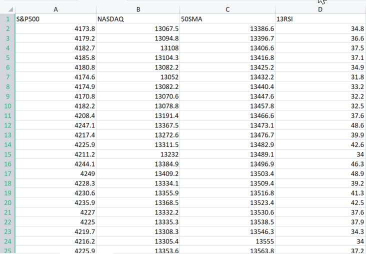
Let's import the dataset
Well I got you covered.
     double XMatrix[]; int rows,cols;

     CSVToMatrix(XMatrix,rows,cols,"NASDAQ_DATA.csv");
     MatrixPrint(XMatrix,cols,3);
The output of the above piece of code:
MN      0       12:02:13.339    NNTestScript (#NQ100,H1)        Matrix
MI      0       12:02:13.340    NNTestScript (#NQ100,H1)        [
MJ      0       12:02:13.340    NNTestScript (#NQ100,H1)         4173.800 13067.500 13386.600    34.800
RD      0       12:02:13.340    NNTestScript (#NQ100,H1)         4179.200 13094.800 13396.700    36.600
JQ      0       12:02:13.340    NNTestScript (#NQ100,H1)         4182.700 13108.000 13406.600    37.500
FK      0       12:02:13.340    NNTestScript (#NQ100,H1)         4185.800 13104.300 13416.800    37.100
.....
.....
.....
DK      0       12:02:13.353    NNTestScript (#NQ100,H1)         4332.700 14090.200 14224.600    43.700
GD      0       12:02:13.353    NNTestScript (#NQ100,H1)         4352.500 14162.000 14225.000    47.300
IN      0       12:02:13.353    NNTestScript (#NQ100,H1)         4401.900 14310.300 14226.200    56.100
DK      0       12:02:13.353    NNTestScript (#NQ100,H1)         4405.200 14312.700 14224.500    56.200
EE      0       12:02:13.353    NNTestScript (#NQ100,H1)         4415.800 14370.400 14223.200    60.000
OS      0       12:02:13.353    NNTestScript (#NQ100,H1)        ]
IE      0       12:02:13.353    NNTestScript (#NQ100,H1)        rows = 744 cols = 4
Now the entire CSV file is stored inside XMatrix[]. Cheers!
The good thing about this resulting matrix is that you no longer have to worry about the inputs of a neural network because the variable cols obtains the number of columns from a Csv file. These are going to be the inputs of a neural network. So finally, here is how the entire script looks like:
//+------------------------------------------------------------------+
//| Script program start function                                    |
//+------------------------------------------------------------------+

#include "NeuralNets.mqh";
CNeuralNets *neuralnet;

//+------------------------------------------------------------------+
void OnStart()
  {

     int hlnodes[3] = {4,6,1};
     int outputs = 1;
     int inputs_=2;

     double XMatrix[]; int rows,cols;

     CSVToMatrix(XMatrix,rows,cols,"NASDAQ_DATA.csv");
     MatrixPrint(XMatrix,cols,3);

     neuralnet = new CNeuralNets(SIGMOID,RELU,cols,hlnodes,outputs);

     neuralnet.train_feedforwardMLP(XMatrix);

     delete(neuralnet);

  }
Simple right? But there are still few lines of code we have to fix, Inside the train_feedforwardMLP, we have add the iterations of the entire dataset in a single epoch iteration, this is to make a complete meaning of an epoch.
       for (int i=0; i<epochs; i++)
         {
           int start = 0;
           int rows = ArraySize(XMatrix)/m_inputs;

             for (int j=0; j<rows; j++) //iterate the entire dataset in a single epoch
               {
                 if (m_debug) printf("<<<< %d >>>",j+1);
                 ArrayCopy(MLPInputs,XMatrix,0,start,m_inputs);

                 FeedForwardMLP(MLPInputs,MLPOutputs,Weights,bias);

                 start+=m_inputs;
               }
         }
Now let's see the logs, when we run this program in debug mode.
bool m_debug = true;
Debug mode may fill up your hard drives space unless you are debugging the neural network kindly set it to false, I ran the program once and I had logs taking up to 21Mb of space.
A brief overview of the two iterations:
MR      0       12:23:16.485    NNTestScript (#NQ100,H1)        <<<< 1 >>>
DE      0       12:23:16.485    NNTestScript (#NQ100,H1)        Hidden layer nodes plus the output
FS      0       12:23:16.485    NNTestScript (#NQ100,H1)        4 6 1 1
KK      0       12:23:16.485    NNTestScript (#NQ100,H1)        Hidden Layer 1 | Nodes 4 | Bias 0.3903
IN      0       12:23:16.485    NNTestScript (#NQ100,H1)        Inputs 4 Weights 16
MJ      0       12:23:16.485    NNTestScript (#NQ100,H1)         4173.80000 13067.50000 13386.60000    34.80000
DF      0       12:23:16.485    NNTestScript (#NQ100,H1)        0.060 0.549 0.797 0.670 0.420 0.914 0.146 0.968 0.464 0.031 0.855 0.240 0.717 0.288 0.372 0.805
....
PD      0       12:23:16.485    NNTestScript (#NQ100,H1)        MLP Final Output
LM      0       12:23:16.485    NNTestScript (#NQ100,H1)        1.333
HP      0       12:23:16.485    NNTestScript (#NQ100,H1)        <<<< 2 >>>
PG      0       12:23:16.485    NNTestScript (#NQ100,H1)        Hidden layer nodes plus the output
JR      0       12:23:16.485    NNTestScript (#NQ100,H1)        4 6 1 1
OH      0       12:23:16.485    NNTestScript (#NQ100,H1)        Hidden Layer 1 | Nodes 4 | Bias 0.3903
EI      0       12:23:16.485    NNTestScript (#NQ100,H1)        Inputs 4 Weights 16
FM      0       12:23:16.485    NNTestScript (#NQ100,H1)         4179.20000 13094.80000 13396.70000    36.60000
II      0       12:23:16.486    NNTestScript (#NQ100,H1)        0.060 0.549 0.797 0.670 0.420 0.914 0.146 0.968 0.464 0.031 0.855 0.240 0.717 0.288 0.372 0.805
GJ      0       12:23:16.486    NNTestScript (#NQ100,H1)
Everything is all set up and working well as expected. Now let's store the model parameter in the binary files.
Storing parameters of the model in a binary file
bool CNeuralNets::WriteBin(double &w[], double &b[])
 {
      string file_name_w = NULL, file_name_b=  NULL;
      int handle_w, handle_b;

      file_name_w = MQLInfoString(MQL_PROGRAM_NAME)+"\\"+"model_w.bin";
      file_name_b =  MQLInfoString(MQL_PROGRAM_NAME)+"\\"+"model_b.bin";

      FileDelete(file_name_w); FileDelete(file_name_b);

       handle_w = FileOpen(file_name_w,FILE_WRITE|FILE_BIN);
       if (handle_w == INVALID_HANDLE)   {  printf("Invalid %s Handle err %d",file_name_w,GetLastError());  }
       else                                 FileWriteArray(handle_w,w);

       FileClose(handle_w);

       handle_b = FileOpen(file_name_b,FILE_WRITE|FILE_BIN);
       if (handle_b == INVALID_HANDLE)   {  printf("Invalid %s Handle err %d",file_name_b,GetLastError());  }
       else                                 FileWriteArray(handle_b,b);

       FileClose(handle_b);

     return(true);
 }
This step is super important. As said earlier, it helps share the model parameters with other programs all using the same library. The binary files will be stored in a subdirectory with the name of your script file:
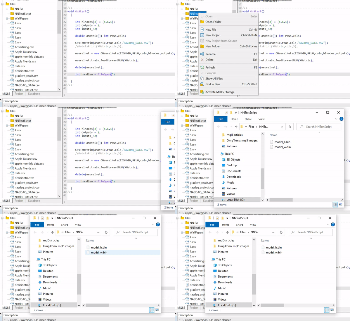
An example on how to access the model parameters in other programs:
     double weights[], bias[];

     int handlew = FileOpen("NNTestScript\\model_w.bin",FILE_READ|FILE_BIN);
     FileReadArray(handlew,weights);
     FileClose(handlew);

     int handleb = FileOpen("NNTestScript\\model_b.bin",FILE_READ|FILE_BIN);
     FileReadArray(handleb,bias);
     FileClose(handleb);

     Print("bias"); ArrayPrint(bias,4);
     Print("Weights"); ArrayPrint(weights,4);
Outputs:
HR      0       14:14:02.380    NNTestScript (#NQ100,H1)        bias
DG      0       14:14:02.385    NNTestScript (#NQ100,H1)        0.0063 0.2737 0.9216 0.4435
OQ      0       14:14:02.385    NNTestScript (#NQ100,H1)        Weights
GG      0       14:14:02.385    NNTestScript (#NQ100,H1)        [ 0] 0.5338 0.6378 0.6710 0.6256 0.8313 0.8093 0.1779 0.4027 0.5229 0.9181 0.5449 0.4888 0.9003 0.2870 0.7107 0.8477
NJ      0       14:14:02.385    NNTestScript (#NQ100,H1)        [16] 0.2328 0.1257 0.4917 0.1930 0.3924 0.2824 0.4536 0.9975 0.9484 0.5822 0.0198 0.7951 0.3904 0.7858 0.7213 0.0529
EN      0       14:14:02.385    NNTestScript (#NQ100,H1)        [32] 0.6332 0.6975 0.9969 0.3987 0.4623 0.4558 0.4474 0.4821 0.0742 0.5364 0.9512 0.2517 0.3690 0.4989 0.5482
Great, you can now access this file from anywhere as long as you know the names and where to find them.
Using the Model
This is the easy part. The feed forward MLP function has been modified, new inputs weights and bias has been added, this will help in running the model for like recent price data or something.
void CNeuralNets::FeedForwardMLP(double &MLPInputs[],double &MLPOutput[],double &Weights[], double &bias[])
Complete code on how to extract the weights and biases and use the model live. First we read the parameters, then we plug in the input values not an input Matrix because this time we use the trained model to predict the outcome of the inputs values. The MLPOutput[] will provide you the output array:
     double weights[], bias[];

     int handlew = FileOpen("NNTestScript\\model_w.bin",FILE_READ|FILE_BIN);
     FileReadArray(handlew,weights);
     FileClose(handlew);

     int handleb = FileOpen("NNTestScript\\model_b.bin",FILE_READ|FILE_BIN);
     FileReadArray(handleb,bias);
     FileClose(handleb);

     double Inputs[]; ArrayCopy(Inputs,XMatrix,0,0,cols); //copy the four first columns from this matrix
     double Output[];

     neuralnet = new CNeuralNets(SIGMOID,RELU,cols,hlnodes,outputs);

     neuralnet.FeedForwardMLP(Inputs,Output,weights,bias);

     Print("Outputs");
     ArrayPrint(Output);

     delete(neuralnet);
This should work fine.
Now, you can feel free to explore various kind of architecture and explore different options to see what works best for you again.
The feedforward neural network was the first and simplest type of artificial neural network devised. In this network, the information moves in only one direction—forward—from the input nodes, through the hidden nodes (if any) and to the output nodes. There are no cycles or loops in the network
This model we just coded is a basic one and may not necessarily provide the results you want unless optimized (I'm 100% sure) hopefully you will be creative and make something out of it.
Final Thoughts
It is important to understand the theory and everything behind closed doors of each machine learning technique because we don't have data science packages in MQL5 at least we have the python frameworks but there are times when we might need to work our way out in MetaTrader, without having a solid understanding on theory behind these kinds of things it will be difficult for one to figure things out and make the most out of machine learning, as we go further the importance of the theory and things we discussed earlier in the article series are proving to be of much importance.
Best Regards.
GitHub repo: https://github.com/MegaJoctan/NeuralNetworks-MQL5
Read more about my library for Matrices and Vectors
Further Reading | Books | References
- Neural Networks for Pattern Recognition (Advanced Texts in Econometrics)
- Neural Networks: Tricks of the Trade (Lecture Notes in Computer Science, 7700)
- Deep Learning (Adaptive Computation and Machine Learning series)
Articles References:
- Data Science and Machine Learning (Part 01): Linear Regression
- Data Science and Machine Learning (Part 02): Logistic Regression
- Data Science and Machine Learning (Part 03): Matrix Regressions
- Data Science and Machine Learning (Part 06): Gradient Descent
- Data Science and Machine Learning — Neural Network (Part 01): Feed Forward Neural Network demystified
Warning: All rights to these materials are reserved by MetaQuotes Ltd. Copying or reprinting of these materials in whole or in part is prohibited.
This article was written by a user of the site and reflects their personal views. MetaQuotes Ltd is not responsible for the accuracy of the information presented, nor for any consequences resulting from the use of the solutions, strategies or recommendations described.
 Neural networks made easy (Part 18): Association rules
 Developing a trading Expert Advisor from scratch (Part 20): New order system (III)
 Learn how to design a trading system by VIDYA
 Developing a trading Expert Advisor from scratch (Part 19): New order system (II)
- Free trading apps
- Over 8,000 signals for copying
- Economic news for exploring financial markets
You agree to website policy and terms of use
Imho, in this cycle the material is much better presented than, for example, in the cycle "Neural Networks - it's simple"...
A question to the admins. Is it possible to insert links to paid bibliographies in the code?
Imho, in this cycle the material is much better presented than, for example, in the cycle "Neural Networks - it's easy"...
A question to the admins. Is it possible to insert links to paid bibliographies in the code?
No, it's not possible, I forgot to remove the link
There is such a thing in the article:
Ok so here is the function responsible for training the neural network.
I am purposely giving an excerpt in the language in which the author wrote the article.
I am embarrassed to ask, where is the learning taking place? Imho, there is direct dissemination taking place....
That's funny:
What if it does? )))
When I saw that there is a section in the article:
Матрицы в помощь
If you suddenly need to change the parameters of a model with static code, optimisation can take a lot of time - it's a headache, backache and other troubles.
I thought that finally someone will describe MO in terms of nativematrices. But the headache from self-made matrices in the form of a one-dimensional array a la XMatrix[] only increased....
4 inputs, 1 hidden laer with 6 neurons and one output?
You don't explain the most important thing well. How to declare the architecture of the model.
How many hidden layers can I use?