
Data Science and ML (Part 45): Forex Time series forecasting using PROPHET by Facebook Model

Contents
- What is a Prophet model
- Understanding the Prophet model
- Implementing the Prophet model in Python
- Adding holidays to the Prophet model
- Making the MetaTrader 5 trading robot based on the Prophet model
- Conclusion
What is a Prophet Model?
The Prophet model is an open-source time series forecasting tool developed by Meta (formerly Facebook). It's designed to provide accurate and user-friendly forecasts for business and analytical purposes, particularly for time series data with strong seasonality and trends.
This model was introduced by Facebook (S. J. Taylor & Benjamin Letham, 2018), originally for forecasting daily data with weekly and yearly seasonality, plus holiday effects. It was later extended to cover more types of seasonal data. It works best with time series that have strong seasonality and several seasons of historical data.
Common terms:
- Trend. The trend shows the tendency of the data to increase or decrease over a long period, and it filters out the seasonal variations.
- Seasonality. Seasonality is the variations that occur over a short period and is not prominent enough to be called a "trend".

In this article, we are going to understand and implement this model given forex data and see how it can help us beat the market but, firstly, let's take a moment to understand this model in detail.
Understanding the Prophet Model
The Prophet model can be considered as a non-linear regression model given by the formula:
![]()
Figure 01
Where:
-
 describes a piecewise-linear trend (or “growth term”)
 -
 describes the various seasonal patterns
 -
 captures the holiday effects, and
  is a white noise error term.
01: The Trend Component
The trend component ![]() allows for changepoints which are automatically selected if not manually specified. These changepoints represents locations in the time when the trend can shift (e.g., sudden growth or decline).
allows for changepoints which are automatically selected if not manually specified. These changepoints represents locations in the time when the trend can shift (e.g., sudden growth or decline).
You can also optionally use logistic growth model instead of a linear one, which introduces a capacity (cap) parameter to model saturation effects. This is useful when growth slows down after reaching a certain natural limit.
02: Seasonality
In the Prophet model, seasonality ![]() is modeled using Fourier series.
is modeled using Fourier series.
By default:
- An order of 10 is used for annual seasonality
- An order 3 is used for weekly seasonality
These Fourier terms help the model capture repeating seasonal effects.
03: The Holiday Effects Part
Holiday effects ![]() are incorporated as dummy variables (one-hot encoded), which allows the model to adjust its forecast around special dates that have historically caused deviations in behaviour. Such as, economic news or public holidays.
are incorporated as dummy variables (one-hot encoded), which allows the model to adjust its forecast around special dates that have historically caused deviations in behaviour. Such as, economic news or public holidays.
The entire model is estimated using a Bayesian framework, which enables automatic selection of the changepoints and other model parameters.
Although this basic decompositional additive model looks simple, the calculation of the terms within this formula is hugely mathematical, so if you don't have a clue about what you are doing, this model can result in making wrong forecasts.
Prophet provides us with two modelling approaches.
- Piecewise Linear Growth Model (default)
- Logistic Growth Model
01. Piecewise Linear Model
This is the default model used by Prophet. It assumes that the trend in the data follows a linear trajectory but may change at specific points in time (called changepoints). This model is suitable for data with steady growth or decline patterns, possibly with abrupt shifts.
This modelling approach is the one represented by the formula in Figure 01.
02. Logistic Growth Model
This model is appropriate for data that shows saturating growth, i.e., it grows rapidly at first, but slows down as it approaches a maximum capacity or limit. This kind of pattern is often seen in real-world systems with natural or business-imposed limits (like user adoption in a saturated market).
The logistic growth model incorporates a capacity parameter that defines this upper limit.
This modelling approach is given by the following formula:

Figure 02
Where:
![]() is the carrying capacity,
is the carrying capacity, ![]() is the growth rate and
is the growth rate and ![]() is an offset parameter.
is an offset parameter.
Implementing the Prophet Model in Python
Using the EURUSD data from the hourly chart, let us attempt to detect the trend, seasonality, and forecast future values using this model.
The first thing you have to do is install all the dependencies from requirements.txt file — attached at the end of this article
pip install -r requirements.txt
Imports.
import pandas as pd
import numpy as np
import MetaTrader5 as mt5
import matplotlib.pyplot as plt
import seaborn as sns
from prophet import Prophet

plt.style.use('fivethirtyeight')
sns.set_style("darkgrid")
Let us get the data from MetaTrader 5.
if not mt5.initialize(r"c:\Program Files\MetaTrader 5 IC Markets (SC)\terminal64.exe"):
    print("Failed to initialize MetaTrader5. Error = ",mt5.last_error())
    mt5.shutdown()

symbol = "EURUSD"
timeframe = mt5.TIMEFRAME_H1

rates = mt5.copy_rates_from_pos(symbol, timeframe, 1, 10000)

if rates is None:
    print(f"Failed to copy rates for symbol={symbol}. MT5 Error = {mt5.last_error()}")
The Prophet model relies heavily on the datetime or date stamp feature. This feature is a must for this model to work.
After receiving the data (rates) from MetaTrader 5, we convert it into a Pandas-DataFrame object. Then, we convert the time column, which contains time in seconds, into a datetime format.
rates_df = pd.DataFrame(rates) # we convert rates object to a dataframe
rates_df["time"] = pd.to_datetime(rates_df["time"], unit="s") # we convert the time from seconds to datatime

rates_df
Outputs.
| time | open | high | low | close | tick_volume | spread | real_volume | |
|---|---|---|---|---|---|---|---|---|
| 0 | 2023-11-10 23:00:00 | 1.06849 | 1.06873 | 1.06826 | 1.06846 | 762 | 0 | 0 |
| 1 | 2023-11-13 00:00:00 | 1.06828 | 1.06853 | 1.06779 | 1.06841 | 1059 | 10 | 0 |
| 2 | 2023-11-13 01:00:00 | 1.06854 | 1.06907 | 1.06854 | 1.06906 | 571 | 0 | 0 |
| 3 | 2023-11-13 02:00:00 | 1.06904 | 1.06904 | 1.06822 | 1.06839 | 1053 | 0 | 0 |
| 4 | 2023-11-13 03:00:00 | 1.06840 | 1.06886 | 1.06811 | 1.06867 | 1204 | 0 | 0 |
The Prophet model is a univariate type of model which requires two features only to operate from a Pandas-DataFrame, i.e., the datetime feature named "ds" (date stamp) and the target variable marked "y" in the dataframe.
For now, let's create a simple dataset from the one received from MetaTrader 5 with two features (time and volatility). This is the data we are going to deploy later to the Prophet model.
prophet_df = pd.DataFrame({
    "time": rates_df["time"],
    "volatility": rates_df["high"] - rates_df["low"]
}).set_index("time")

prophet_df
Volatility (calculated as the difference between high and low price) is our target variable.
Unlike other time series forecasting models such as ARIMA and VAR (discussed previously), which require the target variable to be a stationary variable, the Prophet model is not restricted to this condition. It can work with non-stationary data as well, but all machine learning models tend to perform well with stationary variables as they are easy for models to learn from due to their nature (they have constant mean, variance, and standard deviation).
I chose to work with a stationary target variable for this model to make our life much easier.
Let's plot the DataFrame and observe the features.
# Color pallete for plotting
color_pal = ["#F8766D", "#D39200", "#93AA00",
             "#00BA38", "#00C19F", "#00B9E3",
             "#619CFF", "#DB72FB"]

prophet_df.plot(figsize=(7,5), color=color_pal, title="Volatility (high-low) against time", ylabel="volatility", xlabel="time")
Outputs.
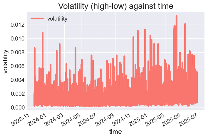
Figure 03
Optionally, we can create X and y features for assessing the impact of time features on the volatility happening in the market.
def create_features(df, label=None):
    """
    Creates time series features from datetime index.
    """

    df = df.copy()
    df['date'] = df.index
    df['hour'] = df['date'].dt.hour
    df['dayofweek'] = df['date'].dt.dayofweek
    df['quarter'] = df['date'].dt.quarter
    df['month'] = df['date'].dt.month
    df['year'] = df['date'].dt.year
    df['dayofyear'] = df['date'].dt.dayofyear
    df['dayofmonth'] = df['date'].dt.day
    df['weekofyear'] = df['date'].dt.isocalendar().week

    X = df[['hour','dayofweek','quarter','month','year',
           'dayofyear','dayofmonth','weekofyear']]
    if label:
        y = df[label]
        return X, y
    return X

X, y = create_features(prophet_df, label='volatility')

features_and_target = pd.concat([X, y], axis=1)
Outputs.
| hour | dayofweek | quarter | month | year | dayofyear | dayofmonth | weekofyear | volatility | |
|---|---|---|---|---|---|---|---|---|---|
| time | |||||||||
| 2023-11-13 16:00:00 | 16 | 0 | 4 | 11 | 2023 | 317 | 13 | 46 | 0.00122 |
| 2023-11-13 17:00:00 | 17 | 0 | 4 | 11 | 2023 | 317 | 13 | 46 | 0.00179 |
| 2023-11-13 18:00:00 | 18 | 0 | 4 | 11 | 2023 | 317 | 13 | 46 | 0.00186 |
| 2023-11-13 19:00:00 | 19 | 0 | 4 | 11 | 2023 | 317 | 13 | 46 | 0.00125 |
| 2023-11-13 20:00:00 | 20 | 0 | 4 | 11 | 2023 | 317 | 13 | 46 | 0.00150 |
We can plot these features against volatility for manual analysis.
sns.pairplot(features_and_target.dropna(),
             hue='hour',
             x_vars=['hour','dayofweek',
                     'year','weekofyear'],
             y_vars='volatility',
             height=5,
             plot_kws={'alpha':0.45, 'linewidth':0.5}
            )

plt.suptitle(f"{symbol} close prices by Hour, Day of Week, Year, and Week")
plt.show()
Outputs.

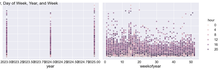
Figure 04
As you can see from the subplots, the hour, day of week, year, and week of year all have an impact on the volatility occurring on every hour of the chart. Knowing this gives us the confidence to proceed using this data for the Prophet model.
Training the Prophet model
We start by splitting the data into training and testing sets using a specific date.
split_date = '01-Jan-2025' # threshold date between training and testing samples, all values after this date are for testing

prophet_df_train = prophet_df.loc[prophet_df.index <= split_date].copy().reset_index().rename(columns={"time": "ds", "volatility": "y"})
prophet_df_test = prophet_df.loc[prophet_df.index > split_date].copy().reset_index().rename(columns={"time": "ds", "volatility": "y"})
We train the Prophet model on the training data.
model = Prophet()
model.fit(prophet_df_train)
After training the model, we often want to test its effectiveness on the out-of-sample data — the information the model hasn't seen before. Unlike other models, the Prophet model has a slightly different way of returning the forecasts.
test_fcst = model.predict(df=prophet_df_test)
Instead of returning a vector containing the predictions, this model returns an entire DataFrame containing various features representing predictions and the state of the model.
test_fcst.head()
Outputs.
	ds      trend   	yhat_lower      yhat_upper      trend_lower     trend_upper     additive_terms  additive_terms_lower    additive_terms_upper    daily   daily_lower     daily_upper     weekly  weekly_lower    weekly_upper    multiplicative_terms    multiplicative_terms_lower      multiplicative_terms_upper      yhat
0       2025-01-02 00:00:00     0.001674        0.000168        0.001993        0.001674        0.001674        -0.000571       -0.000571       -0.000571       -0.000510       -0.000510       -0.000510       -0.000061       -0.000061       -0.000061       0.0     0.0     0.0     0.001102
1       2025-01-02 01:00:00     0.001674        0.000161        0.001977        0.001674        0.001674        -0.000614       -0.000614       -0.000614       -0.000556       -0.000556       -0.000556       -0.000057       -0.000057       -0.000057       0.0     0.0     0.0     0.001060
2       2025-01-02 02:00:00     0.001674        0.000337        0.002123        0.001674        0.001674        -0.000483       -0.000483       -0.000483       -0.000430       -0.000430       -0.000430       -0.000054       -0.000054       -0.000054       0.0     0.0     0.0     0.001191
The following table contains the meaning of some of the columns (features) returned by the predict method.
| Column | Meaning |
|---|---|
| ds | The datetime (timestamp) of the forecasted point |
| yhat | The final forecasted value (what Prophet predicts at that time) |
| yhat_lower, yhat_upper | The lower and upper bounds of the 80% (or 95%) confidence interval for yhat. |
| trend | The value of the trend component at time ds (e.g., slow growth or decline over time. |
| trend_lower, trend_upper | Confidence interval of the trend component |
| additive_terms | The sum of all seasonal + holiday components at time ds (e.g., daily + weekly + holidays) |
| additive_terms_lower, additive_terms_upper | Bounds for additive components. |
| daily | The daily seasonality effect (e.g., hourly patterns in a day) |
| daily_lower, daily_upper | Confidence interval for daily component. |
| weekly | The weekly seasonality effect (e.g., weekends differ from weekdays) |
| weekly_lower, weekly_upper | Confidence interval for the weekly component. |
What we need the most is yhat, yhat_lower, yhat_upper, trend, seasonality patterns (daily, weekly, yearly), holidays (if included), and error bounds for components (*_lower and *_upper) columns.
Let's plot actual and forecasts from the testing sample, alongside the actual values from the training sample.
f, ax = plt.subplots(figsize=(7,5))
ax.scatter(prophet_df_test["ds"], prophet_df_test['y'], color='r') # plot actual values from the testing sample in red

fig = model.plot(test_fcst, ax=ax) # plot the forecasts
Output figure.
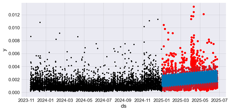
Figure 05
The values in black represent the training sample, the ones in red are the actual values from the testing sample, and the ones in blue are the predictions made by the model for the testing sample.
It is hard to understand the effectiveness of the model by just looking at this plot. Let's create small plots representing actual and forecasts from the testing sample.
Let's evaluate the model in January 2025, the first month in the testing data.
f, ax = plt.subplots(figsize=(7, 5))

ax.scatter(prophet_df_test["ds"], prophet_df_test['y'], color='r')
fig = model.plot(test_fcst, ax=ax)
ax.set_xbound(
            lower=pd.to_datetime("2025-01-01"), # starting data on the x axis
            upper=pd.to_datetime("2025-02-01")) # ending data on the x axis

ax.set_ylim(0, 0.005)
plot = plt.suptitle("January 2025, Actual vs Forecasts")
Outputs.
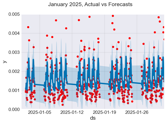
Figure 06
According to what we are seeing on the image above, the Prophet model does get some predictions right, and it doesn't seem to do well with outliers in the data.
Optionally, we can look further into the predictions by analysing the actual values against the predictions made by the model in the first week of January (from January 1st to January 8th).
f, ax = plt.subplots(figsize=(9, 5))

ax.scatter(prophet_df_test["ds"], prophet_df_test['y'], color='r')
fig = model.plot(test_fcst, ax=ax)
ax.set_xbound(
            lower=pd.to_datetime("2025-01-01"),
            upper=pd.to_datetime("2025-01-08"))

ax.set_ylim(0, 0.005)
plot = plt.suptitle("January 01-08, 2025. Actual vs Forecasts")
Outputs.
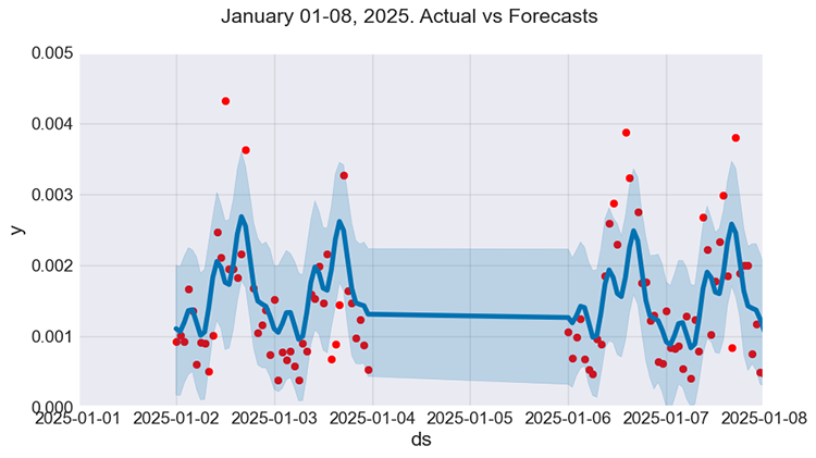
Figure 07
It looks a lot better. However, while the model seems to understand some patterns, its forecasts (predictions) aren't that close to the actual values, something we often strive to achieve when using regression models.
It seems to make a good generalized prediction though.
Let us evaluate it using some evaluation metrics.
import sklearn.metrics as metric

def forecast_accuracy(forecast, actual):
    # Convert to numpy arrays if they aren't already
    forecast = np.asarray(forecast)
    actual = np.asarray(actual)

    metrics = {
        'mape': metric.mean_absolute_percentage_error(actual, forecast),
        'me': np.mean(forecast - actual),  # Mean Error
        'mae': metric.mean_absolute_error(actual, forecast),
        'mpe': np.mean((forecast - actual) / actual),  # Mean Percentage Error
        'rmse': metric.root_mean_squared_error(actual, forecast),
        'minmax': 1 - np.mean(np.minimum(forecast, actual) / np.maximum(forecast, actual)),
        "r2_score": metric.r2_score(forecast, actual)
    }
    return metrics

results = forecast_accuracy(test_pred, prophet_df_test["y"])

for metric_name, value in results.items():
    print(f"{metric_name:<10}: {value:.6f}")
Outputs.
mape      : 0.603277
me        : 0.000130
mae       : 0.000829
mpe       : 0.430299
rmse      : 0.001221
minmax    : 0.339292
r2_score  : -4.547775
What I'm interested in is the MAPE (Mean Absolute Percentage Error) metric; The value of approximately 0.6 means that, on average, the forecasts made by the model are off by 60% from the actual values. Simply put, the model made terrible predictions and it is error prone.
Adding Holidays to the Prophet Model
The Prophet model is built to understand the fact that in any data, there could be events that cause unusual changes in a time series data; these are what we call "holidays".
In the real world, holidays are likely to cause irregular impacts in business data; these can be.
- Public holidays (e.g., New Year’s Day, Christmas)
- Business events (e.g., Black Friday, Product Launch)
- Financial events (e.g., Central bank announcements, quarter ends)
- Local events (e.g., Elections, Weather shocks)
These days don't follow an irregular seasonal pattern, but they repeat, often yearly, quarterly, daily, etc.
In financial (trading) data, we can consider the economic news as holidays, as they cause this scenario described. In doing so, we may help our model address its current issue — failing to capture these extreme values.
As seen in Figure 01 which has the Prophet model's formula, by adding holidays if there are any, makes the model complete as holidays are one of the major building blocks of the formula.
That being said, we have to collect the news using the MQL5 language.
Filename: OHLC + News.mq5
input datetime start_date = D'01.01.2023';
input datetime end_date = D'24.6.2025';
input ENUM_TIMEFRAMES timeframe = PERIOD_H1;

MqlRates rates[];
struct news_data_struct
  {
    datetime time[]; //News release time
    double open[]; //Candle opening price
    double high[]; //Candle high price
    double low[]; //Candle low price
    double close[]; //Candle close price
    string name[]; //Name of the news
    ENUM_CALENDAR_EVENT_SECTOR sector[]; //The sector a news is related to
    ENUM_CALENDAR_EVENT_IMPORTANCE importance[]; //Event importance
    double actual[]; //actual value
    double forecast[]; //forecast value
    double previous[]; //previous value

    void Resize(uint size)
      {
          ArrayResize(time, size);
          ArrayResize(open, size);
          ArrayResize(high, size);
          ArrayResize(low, size);
          ArrayResize(close, size);
          ArrayResize(name, size);
          ArrayResize(sector, size);
          ArrayResize(importance, size);
          ArrayResize(actual, size);
          ArrayResize(forecast, size);
          ArrayResize(previous, size);
      }

  } news_data;
//+------------------------------------------------------------------+
//| Script program start function                                    |
//+------------------------------------------------------------------+
void OnStart()
  {
//---

   if (!ChartSetSymbolPeriod(0, Symbol(), timeframe))
      return;

   SaveNews(StringFormat("%s.%s.OHLC + News.csv",Symbol(),EnumToString(timeframe)));
  }
//+------------------------------------------------------------------+
//|                                                                  |
//|   The function which collects news alongsided OHLC values and    |
//|   saves the data to a CSV file                                   |
//|                                                                  |
//+------------------------------------------------------------------+
void SaveNews(string csv_name)
 {
//--- get OHLC values first

   ResetLastError();
   if (CopyRates(Symbol(), timeframe, start_date, end_date, rates)<=0)
     {
       printf("%s failed to get price information from %s to %s. Error = %d",__FUNCTION__,string(start_date),string(end_date),GetLastError());
       return;
     }

   uint size = rates.Size();
   news_data.Resize(size-1);

//---

   FileDelete(csv_name); //Delete an existing csv file of a given name
   int csv_handle = FileOpen(csv_name,FILE_WRITE|FILE_SHARE_WRITE|FILE_CSV|FILE_ANSI|FILE_COMMON,",",CP_UTF8); //csv handle

   if(csv_handle == INVALID_HANDLE)
     {
       printf("Invalid %s handle Error %d ",csv_name,GetLastError());
       return; //stop the process
     }

   FileSeek(csv_handle,0,SEEK_SET); //go to file begining
   FileWrite(csv_handle,"Time,Open,High,Low,Close,Name,Sector,Importance,Actual,Forecast,Previous"); //write csv header

   MqlCalendarValue values[]; //https://www.mql5.com/en/docs/constants/structures/mqlcalendar#mqlcalendarvalue
   for (uint i=0; i<size-1; i++)
      {
         news_data.time[i] = rates[i].time;
         news_data.open[i] = rates[i].open;
         news_data.high[i] = rates[i].high;
         news_data.low[i] = rates[i].low;
         news_data.close[i] = rates[i].close;

         int all_news = CalendarValueHistory(values, rates[i].time, rates[i+1].time, NULL, NULL); //we obtain all the news with their values https://www.mql5.com/en/docs/calendar/calendarvaluehistory

         for (int n=0; n<all_news; n++)
            {
              MqlCalendarEvent event;
              CalendarEventById(values[n].event_id, event); //Here among all the news we select one after the other by its id https://www.mql5.com/en/docs/calendar/calendareventbyid

              MqlCalendarCountry country; //The couhtry where the currency pair originates
              CalendarCountryById(event.country_id, country); //https://www.mql5.com/en/docs/calendar/calendarcountrybyid

              if (StringFind(Symbol(), country.currency)>-1) //We want to ensure that we filter news that has nothing to do with the base and the quote currency for the current symbol pair
                {
                     news_data.name[i] = event.name;
                     news_data.sector[i] = event.sector;
                     news_data.importance[i] = event.importance;

                     news_data.actual[i] = !MathIsValidNumber(values[n].GetActualValue()) ? 0 : values[n].GetActualValue();
                     news_data.forecast[i] = !MathIsValidNumber(values[n].GetForecastValue()) ? 0 : values[n].GetForecastValue();
                     news_data.previous[i] = !MathIsValidNumber(values[n].GetPreviousValue()) ? 0 : values[n].GetPreviousValue();
                }
            }

          FileWrite(csv_handle,StringFormat("%s,%f,%f,%f,%f,%s,%s,%s,%f,%f,%f",
                                 (string)news_data.time[i],
                                 news_data.open[i],
                                 news_data.high[i],
                                 news_data.low[i],
                                 news_data.close[i],
                                 news_data.name[i],
                                 EnumToString(news_data.sector[i]),
                                 EnumToString(news_data.importance[i]),
                                 news_data.actual[i],
                                 news_data.forecast[i],
                                 news_data.previous[i]
                               ));
       }
//---

   FileClose(csv_handle);
 }
After collecting the news inside the function SaveNews, the data obtained is stored in a CSV file in the "Common path" (folder).
Inside the Python script, we load this data from the same path.
from Trade.TerminalInfo import CTerminalInfo
import os

terminal = CTerminalInfo()
data_path = os.path.join(terminal.common_data_path(), "Files")

timeframe = "PERIOD_H1"
df = pd.read_csv(os.path.join(data_path, f"{symbol}.{timeframe}.OHLC + News.csv"))

df
Outputs.
| Time | Open | High | Low | Close | Name | Sector | Importance | Actual | Forecast | Previous | |
|---|---|---|---|---|---|---|---|---|---|---|---|
| 0 | 2023.01.02 01:00:00 | 1.06967 | 1.06983 | 1.06927 | 1.06983 | New Year's Day | CALENDAR_SECTOR_HOLIDAYS | CALENDAR_IMPORTANCE_NONE | 0.0 | 0.0 | 0.0 |
| 1 | 2023.01.02 02:00:00 | 1.06984 | 1.07059 | 1.06914 | 1.07041 | New Year's Day | CALENDAR_SECTOR_HOLIDAYS | CALENDAR_IMPORTANCE_NONE | 0.0 | 0.0 | 0.0 |
| 2 | 2023.01.02 03:00:00 | 1.07059 | 1.07069 | 1.06858 | 1.06910 | New Year's Day | CALENDAR_SECTOR_HOLIDAYS | CALENDAR_IMPORTANCE_NONE | 0.0 | 0.0 | 0.0 |
| 3 | 2023.01.02 04:00:00 | 1.06909 | 1.06909 | 1.06828 | 1.06880 | New Year's Day | CALENDAR_SECTOR_HOLIDAYS | CALENDAR_IMPORTANCE_NONE | 0.0 | 0.0 | 0.0 |
| 4 | 2023.01.02 05:00:00 | 1.06881 | 1.07029 | 1.06880 | 1.06897 | New Year's Day | CALENDAR_SECTOR_HOLIDAYS | CALENDAR_IMPORTANCE_NONE | 0.0 | 0.0 | 0.0 |
Since we collected the news on every row worth of data in our MQL5 script, we end up with some rows in the news column with the name "(null)" which indicates there were no news at the time, we have to filter these rows.
news_df = df[df['Name'] != "(null)"].copy()
Similary to how we structured the previous data for this model to having two columns — ds and y, we have to ensure the holidays dataset has two columns as well — ds and holiday. The holiday column is for keeping the name of the new(s).
holidays = news_df[['Time', 'Name']].rename(columns={
    'Time': 'ds',
    'Name': 'holiday'
})

holidays['ds'] = pd.to_datetime(holidays['ds'])  # Ensure datetime format
holidays
Outputs.
| ds | holiday | |
|---|---|---|
| 0 | 2023-01-02 01:00:00 | New Year's Day |
| 1 | 2023-01-02 02:00:00 | New Year's Day |
| 2 | 2023-01-02 03:00:00 | New Year's Day |
| 3 | 2023-01-02 04:00:00 | New Year's Day |
| 4 | 2023-01-02 05:00:00 | New Year's Day |
Alongside these features, the holidays dataframe can have two optional columns (lower_window and upper_window). These columns tell the model about the impact of each holiday before and after it occurs.
We know that every holiday in a real world doesn't have the impact on that particular date it occurs, it often has an impact before and after its occurrence(s).
holidays['lower_window'] = 0
holidays['upper_window'] = 1  # Extend effect to 1 hour after
The lower_window column tells how much the holiday impacted the time series data before it occurred, while the upper_window column tells how much the holiday impacted the time series after the time it ocurred.
- For the lower_window column, its values can be less than or equal to zero (<=0), the default value is zero, indicating the holiday doesn't impact any previous value in a timeseries. A value of -1 indicates a certain holiday affects the previous single value of the timeseries before it occurred, etc,.
- For the upper_window column, its values can be greater than or equal to zero (>=0), the default value is zero, indicating the holiday doesn't impact any values in a timeseries after its occurrence. A value of 1 indicates a certain holiday affects the next single value in the time series after it occurred, etc,.
Now, let us add these features as described.
holidays['lower_window'] = -1 # The anticipation of the news affect the volatility 1 bar before it's release
holidays['upper_window'] = 1  # The news affects the volatility 1 bar after its release

holidays
Our holidays DataFrame now becomes:
| ds | holiday | lower_window | upper_window | |
|---|---|---|---|---|
| 0 | 2023-01-02 01:00:00 | New Year's Day | -1 | 1 |
| 1 | 2023-01-02 02:00:00 | New Year's Day | -1 | 1 |
| 2 | 2023-01-02 03:00:00 | New Year's Day | -1 | 1 |
| 3 | 2023-01-02 04:00:00 | New Year's Day | -1 | 1 |
| 4 | 2023-01-02 05:00:00 | New Year's Day | -1 | 1 |
| ... | ... | ... | ... | ... |
| 15369 | 2025-06-20 18:00:00 | Eurogroup Meeting | -1 | 1 |
| 15370 | 2025-06-20 19:00:00 | Eurogroup Meeting | -1 | 1 |
| 15371 | 2025-06-20 20:00:00 | Eurogroup Meeting | -1 | 1 |
| 15372 | 2025-06-20 21:00:00 | Eurogroup Meeting | -1 | 1 |
| 15373 | 2025-06-20 22:00:00 | Eurogroup Meeting | -1 | 1 |
Finally, we give our Prophet model the holidays Dataframe and the training data we prepared previously.
model_w_holidays = Prophet(holidays=holidays)
model_w_holidays.fit(prophet_df_train)
We can test the predictions made by the trained model with holidays by plot the predicted values alongside the actual values as we did prior.
# Predict on training set with model
test_fcst = model_w_holidays.predict(df=prophet_df_test)

test_pred = test_fcst.yhat # We get the predictions

# Plot the forecast with the actuals

f, ax = plt.subplots(figsize=(10,5))
ax.scatter(prophet_df_test["ds"], prophet_df_test['y'], color='r')

fig = model_w_holidays.plot(test_fcst, ax=ax)
Outputs.
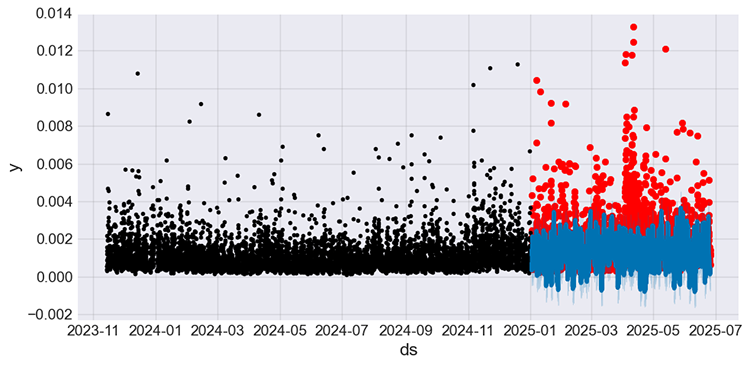
Figure 08
Unlike in the predictions made by the model without news (holidays) in Figure 05 which seems static, the predictions made by this new model with news (holidays) seems to capture some of the fluctuations the prior model was missing.
Again, we evaluate the model using the same metrics we used for the previous model.
results = forecast_accuracy(test_pred, prophet_df_test["y"])

for metric_name, value in results.items():
    print(f"{metric_name:<10}: {value:.6f}")
Outputs.
mape      : 0.549152
me        : -0.000633
mae       : 0.000970
mpe       : -0.175082
rmse      : 0.001487
minmax    : 0.461444
r2_score  : -2.793478
The MAPE metric shows that there is about a 10% improvement in predictions made by the model. The previous model made approximately 60% errors, while this one made around 55% errors. This improvement can also be seen in the r2_score.
The model that makes 55% errors is still not good, an ideal model has to make atleast less than 50% errors (< 50%), we can still do something about the holidays (news) to improve this model.
In this example, we implemented the lower_window and upper_window values as -1 and 1, respectively, meaning the news affects the volatility in the market one bar before and after they were released. While this improved the model, I doubt whether it is ideal or not.
We know that different news could have different impact horizons and strengths, so putting these constant values for all news is fundamentally wrong. Also, we used all news, even the news with lower importance, which we often ignore as traders because such news happen very often and it is hard to measure and observe their impact on the chart.
To fix these two issues, you have to set the lower_window and upper_window values dynamically according to the news type and their observable impact historically.
Example pseudocode.
def get_windows(name):
    if "CPI" in name:
        return (-1, 4) # CPI news affects one previous bar volatility, and it affects the volatility of four bars ahead (4 hours impact forward)
    elif "NFP" in name:
        return (-1, 2) # NFP news affects one previous bar volatility, and it affects the volatility of two bars ahead (2 hours impact afterward)
    elif "FOMC" in name or "Rate" in name:
        return (-2, 6) # NFP news affects two previous bar volatility, and it affects the volatility of six bars ahead (6 hours impact afterward)
    else:
        return (0, 1)  # Default


holidays[['lower_window', 'upper_window']] = holidays['holiday'].apply(
    lambda name: pd.Series(get_windows(name))
)
Given there are tens of thousands of unique news types, and you have to be sure of the impact values implemented, this approach is very difficult to implement but it is the ideal way. So, do the homework :).
For now, the obvious thing we can do is filter some news so that we can remain with news of higher and moderate importance.
news_df = df[
    (df['Name'] != "(null)") & # Filter rows without news at all
    ((df['Importance'] == "CALENDAR_IMPORTANCE_HIGH") | (df['Importance'] == "CALENDAR_IMPORTANCE_MODERATE")) # Filter other news except high importance news
].copy()

news_df
Outputs.
| Time | Open | High | Low | Close | Name | Sector | Importance | Actual | Forecast | Previous | |
|---|---|---|---|---|---|---|---|---|---|---|---|
| 7 | 2023.01.02 08:00:00 | 1.06921 | 1.06973 | 1.06724 | 1.06858 | S&P Global Manufacturing PMI | CALENDAR_SECTOR_BUSINESS | CALENDAR_IMPORTANCE_MODERATE | 47.10 | 47.400 | 47.400 |
| 8 | 2023.01.02 09:00:00 | 1.06878 | 1.06909 | 1.06627 | 1.06784 | S&P Global Manufacturing PMI | CALENDAR_SECTOR_BUSINESS | CALENDAR_IMPORTANCE_MODERATE | 47.80 | 47.800 | 47.800 |
| 31 | 2023.01.03 08:00:00 | 1.06636 | 1.06677 | 1.06514 | 1.06524 | Unemployment | CALENDAR_SECTOR_JOBS | CALENDAR_IMPORTANCE_MODERATE | 2.52 | 2.522 | 2.538 |
| 37 | 2023.01.03 14:00:00 | 1.05283 | 1.05490 | 1.05241 | 1.05355 | S&P Global Manufacturing PMI | CALENDAR_SECTOR_BUSINESS | CALENDAR_IMPORTANCE_HIGH | 46.20 | 46.200 | 46.200 |
| 38 | 2023.01.03 15:00:00 | 1.05353 | 1.05698 | 1.05304 | 1.05602 | Construction Spending m/m | CALENDAR_SECTOR_HOUSING | CALENDAR_IMPORTANCE_MODERATE | 0.20 | 0.200 | -0.300 |
Looks great, after extracting the time and name columns into the holidays Dataframe, we add the lower_window and upper_window values.
holidays = news_df[['Time', 'Name']].rename(columns={
    'Time': 'ds',
    'Name': 'holiday'
})

holidays['ds'] = pd.to_datetime(holidays['ds'])  # Ensure datetime format

holidays['lower_window'] = 0
holidays['upper_window'] = 1

holidays
After training the model, below is the plot showing actual values from both training and testing sample in black and red respectively, and the predictions from the testing sample in blue color.
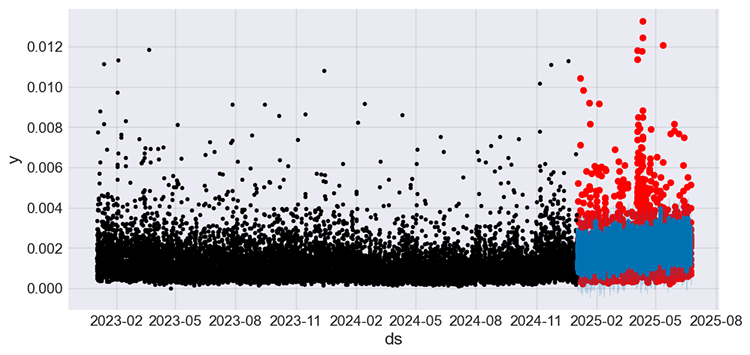
Figure 09
The model improved once more, making approximately 50% errors according to the MAPE metric. We can now use this regression model to make predictions.
mape      : 0.506827
me        : -0.000053
mae       : 0.000783
mpe       : 0.271597
rmse      : 0.001234
minmax    : 0.320422
r2_score  : -3.318859
You might have noticed that we imported the news separately from a CSV file, while we used it alongside the training data imported directly from MetaTrader 5.
The Prophet model aligns (syncs) the dates from the "holidays" DataFrame with the dates in the main training data, as long as the timestamps in the "holidays" DataFrame fall within the training/future prediction period.
Despite this model being capable of syncing the dates, you have to explicitly ensure that both datasets have the same starting dates to get the best out of the two datasets.
I had to go back and modify the process of getting price information from MetaTrader 5 inside main.ipynb, start and end dates now match the ones used inside OHLC + News.mq5 script file.
# set time zone to UTC
timezone = pytz.timezone("Etc/UTC")

# create 'datetime' objects in UTC-time to avoid the implementation of a local time zone offset
utc_from = datetime(2023, 1, 1, tzinfo=timezone)
utc_to = datetime(2025, 6, 24, hour = 0, tzinfo=timezone)

rates = mt5.copy_rates_range(symbol, timeframe, utc_from, utc_to)
Making the MetaTrader 5 Trading Robot based on the Prophet Model
To create a trading robot based on the Prophet model, we have to be able to use it to make real-time predictions on the target variable (volatility in this case) first.
To achieve this, we need a pipeline for obtaining the recent information from the market (symbols), including the latest news updates all at once. In the training script main.ipynb, we collected data from MetaTrader 5 using MetaTrader 5-Python package but, this package doesn't offer a way to get news so, we definitely need to use MQL5 for this process.
The idea is to exchange data between the Python script (trading robot) and an Expert Advisor (EA) in MQL5.
- An EA (Data for Prophet.mq5) attached to the MetaTrader 5 chart periodically saves the data (News and OHLC values) from MetaTrader 5 to a CSV file in the common folder.
- This file is then read by the Python script (Prophet-trading-bot.py) for training the Prophet model periodically.
- After training, the model is then used for making predictions that are then used for making trading decisions inside the same Python script.
Filename: Data for Prophet.mq5
input uint collect_news_interval_seconds = 60;
input uint training_bars = 1000;

input ENUM_TIMEFRAMES timeframe = PERIOD_H1;
//... other lines of code
//+------------------------------------------------------------------+
//| Expert initialization function                                   |
//+------------------------------------------------------------------+
int OnInit()
  {
//--- create timer

   EventSetTimer(collect_news_interval_seconds);

   if (!ChartSetSymbolPeriod(0, Symbol(), timeframe))
      return INIT_FAILED;
//---
   return(INIT_SUCCEEDED);
  }
//+------------------------------------------------------------------+
//| Expert deinitialization function                                 |
//+------------------------------------------------------------------+
void OnDeinit(const int reason)
  {
//--- destroy timer
   EventKillTimer();
  }
//+------------------------------------------------------------------+
//| Expert tick function                                             |
//+------------------------------------------------------------------+
void OnTick()
  {
//---
  }
//+------------------------------------------------------------------+
//| Timer function                                                   |
//+------------------------------------------------------------------+
void OnTimer()
  {
//---
   MqlDateTime time_struct;
   TimeToStruct(TimeGMT(), time_struct);

   SaveNews(StringFormat("%s.%s.OHLC.date=%s.hour=%d + News.csv",Symbol(),EnumToString(timeframe), TimeToString(TimeGMT(), TIME_DATE), time_struct.hour));
  }
To ensure that we are working with the right file, the date and current hour (in UTC Time) are used in naming the CSV file.
This Expert advisor collects news and other values and saves them to a CSV file on every minute by default, according to the OnTimer function.
Inside a Python script, we load the CSV file from the common folder the same way, and import the data.
Filename: Prophet-trading-bot.py
def prophet_vol_predict() -> float:

    # Getting the data with news

    now_utc = datetime.utcnow()
    current_date = now_utc.strftime("%Y.%m.%d")
    current_hour = now_utc.hour

    filename = f"{symbol}.{timeframe}.OHLC.date={current_date}.hour={current_hour} + News.csv" # the same file naming as in MQL5 script
    common_path = os.path.join(terminal.common_data_path(), "Files")
    csv_path = os.path.join(common_path, filename)

    # Keep trying to read a CSV file until it is found, as there could be a temporary difference in values for the file due to the change in time
    while True:
        if os.path.exists(csv_path):
            try:
                rates_df = pd.read_csv(csv_path)
                rates_df["Time"] = pd.to_datetime(rates_df["Time"], unit="s", errors="ignore")  # Convert time from seconds to datetime

                print("File loaded successfully.")
                break  # Exit the loop once file is read
            except Exception as e:
                print(f"Error reading the file: {e}")
                time.sleep(30)
        else:
            print("File not found. Retrying in 30 seconds...")
            time.sleep(30)
We prepare the volatility column and extract the news names for the training data and the holidays data, respectively.
# Getting continous variables for the prophet model

prophet_df = pd.DataFrame({
    "time": rates_df["Time"],
    "volatility": rates_df["High"] - rates_df["Low"]
}).set_index("time")

prophet_df = prophet_df.reset_index().rename(columns={"time": "ds", "volatility": "y"}).copy()

print("Prophet df\n",prophet_df.head())

# Getting the news data for the model as well

news_df = rates_df[
    (rates_df['Name'] != "(null)") & # Filter rows without news at all
    ((rates_df['Importance'] == "CALENDAR_IMPORTANCE_HIGH") | (rates_df['Importance'] == "CALENDAR_IMPORTANCE_MODERATE")) # Filter other news except high importance news
].copy()

holidays = news_df[['Time', 'Name']].rename(columns={
    'Time': 'ds',
    'Name': 'holiday'
})

holidays['ds'] = pd.to_datetime(holidays['ds'])  # Ensure datetime format

holidays['lower_window'] = 0
holidays['upper_window'] = 1

print("Holidays df\n", holidays)
At the end of the function prophet_vol_pred, we train the model with the received information and return a single predicted value, which represents the predicted volatility the model thinks is going to happen in the next bar on the market.
    # re-training the prophet model

    prophet_model = Prophet(holidays=holidays)
    prophet_model.fit(prophet_df)

    # Making future predictions

    future = prophet_model.make_future_dataframe(periods=1) # prepare the dataframe for a single value prediction
    forecast = prophet_model.predict(future) # Predict the next one value

    return forecast.yhat[0] # return a single predicted value
Similarly to other machine learning models used in time series forecasting, we have to update them very often to ensure they are equipped with the recent information which is relevant to future forecasts (predictions). This is the main reason to why we retrain the model before making any new predictions.
Let's run the function and observe the outcome.
print("predicted volatility: ",prophet_vol_predict())
Outputs.
File loaded successfully.
Prophet df
                     ds        y
0  2025.04.29 01:00:00  0.00100
1  2025.04.29 02:00:00  0.00210
2  2025.04.29 03:00:00  0.00170
3  2025.04.29 04:00:00  0.00215
4  2025.04.29 05:00:00  0.00278
Holidays df
                      ds                                     holiday  lower_window  upper_window
8   2025-04-29 09:00:00                        GfK Consumer Climate             0             1
14  2025-04-29 15:00:00          Retail Inventories excl. Autos m/m             0             1
31  2025-04-30 08:00:00                       Consumer Spending m/m             0             1
33  2025-04-30 10:00:00                                Unemployment             0             1
35  2025-04-30 12:00:00                                     GDP y/y             0             1
..                  ...                                         ...           ...           ...
978 2025-06-24 19:00:00                 FOMC Member Williams Speech             0             1
979 2025-06-24 20:00:00                         2-Year Note Auction             0             1
982 2025-06-24 23:00:00  Fed Vice Chair for Supervision Barr Speech             0             1
984 2025-06-25 01:00:00                            Jobseekers Total             0             1
994 2025-06-25 11:00:00  Bbk Executive Board Member Mauderer Speech             0             1

[186 rows x 4 columns]
16:01:50 - cmdstanpy - INFO - Chain [1] start processing
16:01:50 - cmdstanpy - INFO - Chain [1] done processing
predicted volatility:  0.0013592111956094713
Now that we are capable of getting the predicted value, we can use it in our trading strategy.
symbol = "EURUSD"
timeframe = "PERIOD_H1"
terminal = CTerminalInfo()
m_position = CPositionInfo()

def main():

    m_symbol = CSymbolInfo(symbol=symbol)

    magic_number = 25062025
    slippage = 100

    m_trade = CTrade(magic_number=magic_number,
                     filling_type_symbol=symbol,
                     deviation_points=slippage)

    m_symbol.refresh_rates() # Get recent information from the market

    # we want to open random buy and sell trades if they don't exist and use the predicted volatility to set our stoploss and takeprofit targets

    predicted_volatility = prophet_vol_predict()
    print("predicted volatility: ",prophet_vol_predict())

    if pos_exists(mt5.POSITION_TYPE_BUY, magic_number, symbol) is False:
        m_trade.buy(volume=m_symbol.lots_min(),
                    symbol=symbol,
                    price=m_symbol.ask(),
                    sl=m_symbol.ask()-predicted_volatility,
                    tp=m_symbol.ask()+predicted_volatility)

    if pos_exists(mt5.POSITION_TYPE_SELL, magic_number, symbol) is False:
        m_trade.sell(volume=m_symbol.lots_min(),
                     symbol=symbol,
                     price=m_symbol.bid(),
                     sl=m_symbol.bid()+predicted_volatility,
                     tp=m_symbol.bid()-predicted_volatility)
The above function gets the predicted volatility from the Prophet model and uses it for setting stoploss and takeprofit targets in our trades. Before opening a random trade, it checks if a position (trade) of the same type doesn't exist before opening one.
Function call.
main()
Outcome.
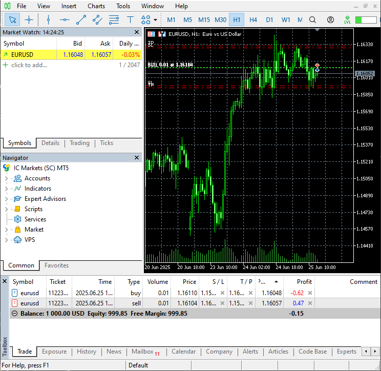
Figure 10
Two opposite trades were opened in MetaTrader 5 with stop loss and take profit values which is the volatility predicted by the model.
We can automate this training process and monitor trading operations and signals regularly.
schedule.every(1).minute.do(main) # train and run trading operations after every one minute

while True:

    schedule.run_pending()
    time.sleep(1)
Conclusion
While some articles, posts, and tutorials online claim that the Prophet model is good for time series forecasting, I think it is one of the worst models we have discussed in this article series.
It might be good in forecasting some simple time series problems like predicting the demand of some business which depends on the weather, holidays or, some kind of seasonal patterns but, financial markets are much complex than that, as seen in the figures (05, 06, 07, 08, 09) illustrating actual and predicted values on the testing samples. The Prophet model fails to get the majority of the predictions near the actual values.
I understand that there are certain things you can do to improve it, but I would suggest using it on simple problems for now.
Summarized limitations of this model include.
- Simple model structure which doesn't support complex interactions
- Not great with volatility — as seen above, it doesn't do well with forex data.
- No multivariate modelling — It supports two features: time and the target variable.
- No cross validation or hyperparameter tuning ability as you have to control trend, seasonality, and changepoints yourself.
Best regards.
Sources & references
- https://facebook.github.io/prophet/
- https://otexts.com/fpp3/prophet.html
- https://www.geeksforgeeks.org/time-series-analysis-using-facebook-prophet/
- https://www.kaggle.com/code/omegajoctan/time-series-forecasting-with-prophet/edit
Attachments Table
| Filename | Description & Usage |
|---|---|
| Python code\main.ipynb | A Jupyter notebook for data analysis and exploration of the Prophet model. |
| Python code\Prophet-trading-bot.py | MetaTrader 5 Python-based trading robot. |
| Python code\requirementx.txt | A text file containing Python dependencies and their version number |
| Python code\error_description.py | Contains the description of all error codes produced by MetaTrader 5. |
| Python code\Trade\* | Contains the Trade classes (CTrade, CPositionInfo, etc.) for Python, similar to the ones available in the MQL5 language. |
| Experts\Data for Prophet.mq5 | An expert advisor that periodically collects and stores the data for training the Prophet model to a CSV file |
| Scripts\OHLC + News.mq5 | A script for collecting and storing in a CSV file the data for training the Prophet model. |
Warning: All rights to these materials are reserved by MetaQuotes Ltd. Copying or reprinting of these materials in whole or in part is prohibited.
This article was written by a user of the site and reflects their personal views. MetaQuotes Ltd is not responsible for the accuracy of the information presented, nor for any consequences resulting from the use of the solutions, strategies or recommendations described.

- Free trading apps
- Over 8,000 signals for copying
- Economic news for exploring financial markets
You agree to website policy and terms of use