Data Science and Machine Learning (Part 03): Matrix Regressions

After a long period of trials and errors finally, the puzzle of multiple dynamic regression is solved... keep reading.
If you paid attention to the previous two articles you'll notice the big issue I had is programming models that could handle more independent variables, by this I mean dynamically handle more inputs because when it comes to creating strategies we are going to deal with hundreds of data, so we want to be sure that our models can cope with this demand.

Matrix
For those that skipped mathematics classes, a matrix is a rectangular array or table of numbers or other mathematical objects arranged in rows and columns which is used to represent a mathematical object or a property of such an object.
For example:

Elephant in the room.
The way we read the matrices is rows x columns. The above matrix is a 2x3 matrix meaning 2 rows, 3 columns.
It is no doubt that matrices play a huge part in how modern computers process information and compute large numbers, the main reason why they are able to achieve such a thing is because data in matrix is stored in the array form that computers can read and manipulate. So let's see their application in machine learning.
Linear Regression
Matrices allow computations in linear algebra. Therefore, the study of matrices is a large part of linear algebra, so we can use matrices to make our linear regression models.
As we all know, the equation of a straight line is

where, ∈ is error terms, Bo and Bi are the coefficients y-intercept and slope coefficient respectively
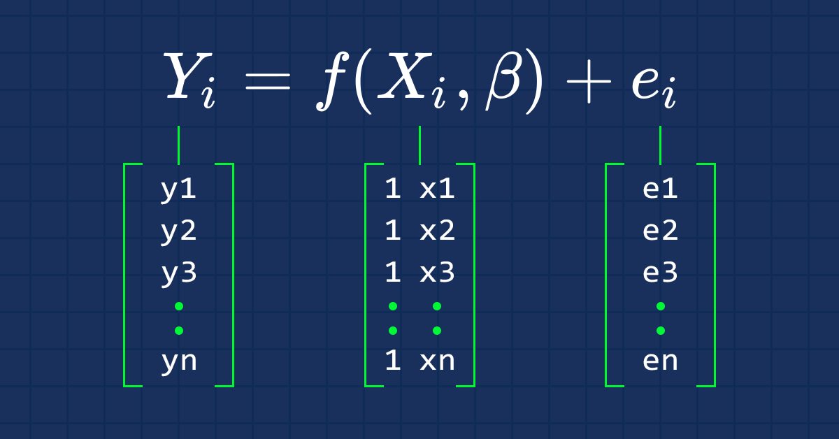
What we are interested in these article series from now on is the vector form of an equation. Here it is

This is the formulation of a simple linear regression in a matrix form.
For a simple linear model (and other regression models) we are usually interested in finding the slope coefficients/ ordinary least square estimators.
The vector Beta is a vector containing betas.
Bo and B1, as explained from the equation

We are interested in finding the coefficients since they are very essential in building a model.
The formula for the estimators of the models in vector form is

This is a very important formula for all the nerds out there to memorize. We will discuss how to find the elements on the formula shortly.
The Product of xTx will give out the symmetric matrix since the number of columns in xT is the same as the number of rows in x, we'll see this later in action.
As said earlier, x is also referred to as a design matrix, here is how its matrix will look like.
Design Matrix

As you can see that on the very first column we have put just the values of 1 all the way to the end of our rows in a Matrix array. This is the first step to preparing our data for Matrix regression you will see the advantages of doing such a thing as we go further into calculations.
We handle this process in the Init() function of our library.
void CSimpleMatLinearRegression::Init(double &x[],double &y[], bool debugmode=true)
 {
    ArrayResize(Betas,2); //since it is simple linear Regression we only have two variables x and y

    if (ArraySize(x) != ArraySize(y))
      Alert("There is variance in the number of independent variables and dependent variables \n Calculations may fall short");

    m_rowsize = ArraySize(x);

    ArrayResize(m_xvalues,m_rowsize+m_rowsize); //add one row size space for the filled values
    ArrayFill(m_xvalues,0,m_rowsize,1); //fill the first row with one(s) here is where the operation is performed

    ArrayCopy(m_xvalues,x,m_rowsize,0,WHOLE_ARRAY); //add x values to the array starting where the filled values ended
    ArrayCopy(m_yvalues,y);

    m_debug=debugmode;
 }
To this point when we print the design matrix values here is our output, as you can see just where the filled values of one ends in a row its where the x values starts.
[ 0] 1.0 1.0 1.0 1.0 1.0 1.0 1.0 1.0 1.0 1.0 1.0 1.0 1.0 1.0 1.0 1.0 1.0 1.0 1.0 1.0 1.0
[ 21] 1.0 1.0 1.0 1.0 1.0 1.0 1.0 1.0 1.0 1.0 1.0 1.0 1.0 1.0 1.0 1.0 1.0 1.0 1.0 1.0 1.0
........
........
[ 693] 1.0 1.0 1.0 1.0 1.0 1.0 1.0 1.0 1.0 1.0 1.0 1.0 1.0 1.0 1.0 1.0 1.0 1.0 1.0 1.0 1.0
[ 714] 1.0 1.0 1.0 1.0 1.0 1.0 1.0 1.0 1.0 1.0 1.0 1.0 1.0 1.0 1.0 1.0 1.0 1.0 1.0 1.0 1.0
[ 735] 1.0 1.0 1.0 1.0 1.0 1.0 1.0 1.0 1.0 4173.8 4179.2 4182.7 4185.8 4180.8 4174.6 4174.9 4170.8 4182.2 4208.4 4247.1 4217.4
[ 756] 4225.9 4211.2 4244.1 4249.0 4228.3 4230.6 4235.9 4227.0 4225.0 4219.7 4216.2 4225.9 4229.9 4232.8 4226.4 4206.9 4204.6 4234.7 4240.7 4243.4 4247.7
........
........
[1449] 4436.4 4442.2 4439.5 4442.5 4436.2 4423.6 4416.8 4419.6 4427.0 4431.7 4372.7 4374.6 4357.9 4381.6 4345.8 4296.8 4321.0 4284.6 4310.9 4318.1 4328.0
[1470] 4334.0 4352.3 4350.6 4354.0 4340.1 4347.5 4361.3 4345.9 4346.5 4342.8 4351.7 4326.0 4323.2 4332.7 4352.5 4401.9 4405.2 4415.8
xT or x transpose is the process in Matrix by which, we swap the rows with the columns.

This means that if we multiply these two matrices

We will skip the process of transposing a matrix because the way we collected our data is in already transposed form, although we have to untranspose the x values on the other hand so that we can multiply them with the already transposed x Matrix.
Just a shoutout, the matrix nx2 that is not transposed array will look like [1 x1 1 x2 1 ... 1 xn]. Let's see this in action.
Un-transposing the X Matrix
Our Matrix in transposed form, that was obtained from a csv file looks like this, when printed out:
Transposed Matrix
[
[ 0] 1 1 1 1 1 1 1 1 1 1 1 1 1 1 1 1 1 1 1 1 1 1 1 1 1 1 1 1 1 1 1 1 1 1 1 1 1 1 1 1 1 1 1 1 1 1 1 1 1 1
...
...
[ 0] 4174 4179 4183 4186 4181 4175 4175 4171 4182 4208 4247 4217 4226 4211 4244 4249 4228 4231 4236 4227 4225 4220 4216 4226
...
...
[720] 4297 4321 4285 4311 4318 4328 4334 4352 4351 4354 4340 4348 4361 4346 4346 4343 4352 4326 4323 4333 4352 4402 4405 4416
]
The Process of un-transposing it, we just have to swap the rows with the columns, the same-opposite process as transposing the matrix.
    int tr_rows = m_rowsize,
        tr_cols = 1+1; //since we have one independent variable we add one for the space created by those values of one


    MatrixUnTranspose(m_xvalues,tr_cols,tr_rows);

    Print("UnTransposed Matrix");
    MatrixPrint(m_xvalues,tr_cols,tr_rows);
Things get tricky here.

We put the columns from a transposed matrix in a place where is supposed to be rows and rows a place where columns are needed, the output upon running this code snippet will be:
        UnTransposed Matrix
        [
            1  4248
            1  4201
            1  4352
            1  4402
...
...
            1  4405
            1  4416
        ]
xT is a 2xn matrix, x is an nx2. The resulting matrix will be a 2x2 matrix
So let's work out to see what the product of their multiplication will look like.
Attention: for matrix multiplication to become possible the number of columns in the first matrix must be the equal to the number of rows in the second matrix.
See matrix multiplication rules on this link https://en.wikipedia.org/wiki/Matrix_multiplication.
The way multiplication is performed in this matrix is:
- Row 1 times column 1
- Row 1 times column 2
- Row 2 times column 1
- Row 2 times column 2
From our matrices row 1 time column1, the output will be the summation of the product of row1 which contains the values of one and the product of column1 which also contains the values of one this is no different than incrementing the value of one by one on each iteration.

Note:
If you would like to know the number of observations in your dataset you can rely on the number on the first row first column in the output of xTx.
Row 1 times column 2. Since row 1 contains the values of ones when we sum the product of row1 (which is values of one) and column2(which is values of x), the output will be the summation of x items since one will have no effect to the multiplication.

Row2 times column 1. The output will be the summation of x since the values of one from row2 have no effect when they multiply the x values that are on the column 1.

The last part will be the summation of x values when squared.
Since it is the summation of the product of row2 which contains x values and colum2 which also contains x values

As you can see, the output of the matrix is a 2x2 matrix in this case.
Let's see how this works in the real world, using the data set from our very first article in Linear regression https://www.mql5.com/en/articles/10459. Let's extracts the data and put it in an array x for independent variable and y for dependent variables.
//inside MatrixRegTest.mq5 script

#include "MatrixRegression.mqh";
#include "LinearRegressionLib.mqh";
CSimpleMatLinearRegression matlr;
CSimpleLinearRegression lr;
//+------------------------------------------------------------------+
//| Script program start function                                    |
//+------------------------------------------------------------------+
void OnStart()
  {
    //double x[] = {651,762,856,1063,1190,1298,1421,1440,1518}; //stands for sales
    //double y[] = {23,26,30,34,43,48,52,57,58}; //money spent on ads
//---
    double x[], y[];
    string file_name = "NASDAQ_DATA.csv", delimiter = ",";

    lr.GetDataToArray(x,file_name,delimiter,1);
    lr.GetDataToArray(y,file_name,delimiter,2);

}
I have imported the CsimpleLinearRegression library that we created in the first article here
CSimpleLinearRegression lr;
because there are certain functions that we might want to use, like getting data to arrays.
Let's find xTx
MatrixMultiply(xT,m_xvalues,xTx,tr_cols,tr_rows,tr_rows,tr_cols);

Print("xTx");
MatrixPrint(xTx,tr_cols,tr_cols,5); //remember?? the output of the matrix will be the row1 and col2 marked in red
If you pay attention to the array xT[], you can see we just copied the x values and stored them in this xT[] array just for clarification, as I said earlier the way we collected data from our csv file to an array using the Function GetDataToArray() gives us data that is already transposed.
We then multiplied the array xT[] with m_xvalues[] which are now untranposed, m_xvalues is the global defined array for our x values in this library. This is the inside of our MatrixMultiply() function.
void CSimpleMatLinearRegression::MatrixMultiply(double &A[],double &B[],double &output_arr[],int row1,int col1,int row2,int col2)
 {
//---
   double MultPl_Mat[]; //where the multiplications will be stored

   if (col1 != row2)
        Alert("Matrix Multiplication Error, \n The number of columns in the first matrix is not equal to the number of rows in second matrix");

   else
    {
        ArrayResize(MultPl_Mat,row1*col2);

        int mat1_index, mat2_index;

        if (col1==1)  //Multiplication for 1D Array
         {
            for (int i=0; i<row1; i++)
              for(int k=0; k<row1; k++)
                 {
                   int index = k + (i*row1);
                   MultPl_Mat[index] = A[i] * B[k];
                 }
           //Print("Matrix Multiplication output");
           //ArrayPrint(MultPl_Mat);
         }
        else
         {
         //if the matrix has more than 2 dimensionals
         for (int i=0; i<row1; i++)
          for (int j=0; j<col2; j++)
            {
               int index = j + (i*col2);
               MultPl_Mat[index] = 0;

               for (int k=0; k<col1; k++)
                 {
                     mat1_index = k + (i*row2);   //k + (i*row2)
                     mat2_index = j + (k*col2);   //j + (k*col2)

                     //Print("index out ",index," index a ",mat1_index," index b ",mat2_index);

                       MultPl_Mat[index] += A[mat1_index] * B[mat2_index];
                       DBL_MAX_MIN(MultPl_Mat[index]);
                 }
               //Print(index," ",MultPl_Mat[index]);
             }
           ArrayCopy(output_arr,MultPl_Mat);
           ArrayFree(MultPl_Mat);
       }
    }
 }
To be honest this multiplication looks confusing and ugly especially when things like
k + (i*row2);
j + (k*col2);
have been used. Relax, bro! The way I have manipulated those indexes is so that they can give us the index at a specific row and column. This could be easily understandable if I could have used two dimensional arrays for example Matrix[rows][columns] which would be Matrix[i][k] in this case but I chose not to because multi dimensional arrays have limitations so I had to find a way through. I have simple c++ code linked at the end of the article that I think would help you understand how I did this or you can read to this blog to understand more about that https://www.programiz.com/cpp-programming/examples/matrix-multiplication.
The output of successfully function xTx using a MatrixPrint() function will be
 Print("xTx");
 MatrixPrint(xTx,tr_cols,tr_cols,5);
xTx
[
    744.00000 3257845.70000
    3257845.70000 14275586746.32998

]
As you can see the first element in our xTx array has the number of observations for each data in our dataset, this is why filling the design matrix with values of one initially on the very first column is very important.
Now let's find the Inverse of the xTx matrix.
Inverse of xTx Matrix
To find the inverse of a 2x2 Matrix, we first swap the first and the last elements of the diagonal, then we add negative signs to the other two values.
The formula is as given on the image below:

To find the determinant of a matrix det(xTx) = Product of the first diagonal - Product of the second diagonal.
Here is how we can find the inverse in mql5 code
void CSimpleMatLinearRegression::MatrixInverse(double &Matrix[],double &output_mat[])
{
// According to Matrix Rules the Inverse of a matrix can only be found when the
// Matrix is Identical Starting from a 2x2 matrix so this is our starting point

   int matrix_size = ArraySize(Matrix);

   if (matrix_size > 4)
     Print("Matrix allowed using this method is a 2x2 matrix Only");

  if (matrix_size==4)
     {
       MatrixtypeSquare(matrix_size);
       //first step is we swap the first and the last value of the matrix
       //so far we know that the last value is equal to arraysize minus one
       int last_mat = matrix_size-1;

       ArrayCopy(output_mat,Matrix);

       // first diagonal
       output_mat[0] = Matrix[last_mat]; //swap first array with last one
       output_mat[last_mat] = Matrix[0]; //swap the last array with the first one
       double first_diagonal = output_mat[0]*output_mat[last_mat];

       // second diagonal  //adiing negative signs >>>
       output_mat[1] = - Matrix[1];
       output_mat[2] = - Matrix[2];
       double second_diagonal = output_mat[1]*output_mat[2];

       if (m_debug)
        {
          Print("Diagonal already Swapped Matrix");
          MatrixPrint(output_mat,2,2);
        }

       //formula for inverse is 1/det(xTx) * (xtx)-1
       //determinant equals the product of the first diagonal minus the product of the second diagonal

       double det =  first_diagonal-second_diagonal;

       if (m_debug)
       Print("determinant =",det);


       for (int i=0; i<matrix_size; i++)
          { output_mat[i] = output_mat[i]*(1/det); DBL_MAX_MIN(output_mat[i]); }

     }
 }
The output of running this block of code will be
	Diagonal already Swapped Matrix
	[
	 14275586746     -3257846
	 -3257846       744
	]
	determinant =7477934261.0234375
Let's print the Inverse of the Matrix to see how it looks like
       Print("inverse xtx");
       MatrixPrint(inverse_xTx,2,2,_digits); //inverse of simple lr will always be a 2x2 matrix
The output will surely be
[
1.9090281 -0.0004357
-0.0004357 0.0000001
]
Now we have the xTx inverse let's move on to.
Finding xTy
Here we multiply xT[] with the y[] values
    double xTy[];
    MatrixMultiply(xT,m_yvalues,xTy,tr_cols,tr_rows,tr_rows,1); //1 at the end is because the y values matrix will always have one column which is it

    Print("xTy");
    MatrixPrint(xTy,tr_rows,1,_digits); //remember again??? how we find the output of our matrix row1 x column2
The output will surely be
xTy
[
10550016.7000000 46241904488.2699585
]
Refer to the formula
Now that we have xTx inverse and xTy let's wrap things up.

   MatrixMultiply(inverse_xTx,xTy,Betas,2,2,2,1); //inverse is a square 2x2 matrix while xty is a 2x1


   Print("coefficients");
   MatrixPrint(Betas,2,1,5); // for simple lr our betas matrix will be a 2x1
More details about how we called the function.
The output of this code snippet will be
coefficients
[
-5524.40278 4.49996
]
B A M !!! This is the same result on coefficients that we were able to obtain with our model in scalar form, in Part 01 of these article series.
The number at the first index of the Array Betas will always be the Constant/ Y- Intercept. The reason we are able to obtain it initially is because we filled the design matrix with the values of one to the first column, again this is showing how important that process is. It leaves the space for the y - intercept to stay in that column.
Now, we are done with Simple Linear Regression. Lets see what multiple regression will look like. Pay close attention because things can get tricky and complicated and times.
Multiple Dynamic Regression Puzzle Solved
The good thing about building our models based on the matrix is that it is easy to scale them up the without having to change the code much when it comes to building the model. The significant change that you will notice on multiple regression is how the inverse of a matrix is found because this is the hardest part which I have spent a long time trying to figure out, I will in details later when we reach that section but for now, let's code the things that we might need in our MultipleMatrixRegression library.
We could have just the one library that could handle simple and multiple regression all by letting us just input the function arguments but I have decided to create another file so as to clarify things, since the process will be nearly the same as long as you have understood the calculations we have performed under our simple linear regression section I just explained.
First things first, let's code the basic things that we might need in our library.
class CMultipleMatLinearReg
  {
      private:

                           int     m_handle;
                           string  m_filename;
                           string  DataColumnNames[];    //store the column names from csv file
                           int     rows_total;
                           int     x_columns_chosen;     //Number of x columns chosen

                           bool    m_debug;
                           double  m_yvalues[];     //y values or dependent values matrix
                           double  m_allxvalues[];  //All x values design matrix
                           string  m_XColsArray[];  //store the x columns chosen on the Init
                           string  m_delimiter;

                           double  Betas[]; //Array for storing the coefficients

      protected:

                           bool    fileopen();
                           void    GetAllDataToArray(double& array[]);
                           void    GetColumnDatatoArray(int from_column_number, double &toArr[]);
      public:

                           CMultipleMatLinearReg(void);
                          ~CMultipleMatLinearReg(void);

                           void Init(int y_column, string x_columns="", string filename = NULL, string delimiter = ",", bool debugmode=true);
  };
This is what happens inside the Init() function
void CMultipleMatLinearReg::Init(int y_column,string x_columns="",string filename=NULL,string delimiter=",",bool debugmode=true)
 {
//--- pass some inputs to the global inputs since they are reusable

   m_filename = filename;
   m_debug = debugmode;
   m_delimiter = delimiter;

//---

   ushort separator = StringGetCharacter(m_delimiter,0);
   StringSplit(x_columns,separator,m_XColsArray);
   x_columns_chosen = ArraySize(m_XColsArray);
   ArrayResize(DataColumnNames,x_columns_chosen);

//---

   if (m_debug)
    {
      Print("Init, number of X columns chosen =",x_columns_chosen);
      ArrayPrint(m_XColsArray);
    }

//---

   GetAllDataToArray(m_allxvalues);
   GetColumnDatatoArray(y_column,m_yvalues);


// check for variance in the data set by dividing the rows total size by the number of x columns selected, there shouldn't be a reminder

   if (rows_total % x_columns_chosen != 0)
     Alert("There are variance(s) in your dataset columns sizes, This may Lead to Incorrect calculations");
   else
     {
      //--- Refill the first row of a design matrix with the values of 1
       int single_rowsize = rows_total/x_columns_chosen;
       double Temp_x[]; //Temporary x array

       ArrayResize(Temp_x,single_rowsize);
       ArrayFill(Temp_x,0,single_rowsize,1);
       ArrayCopy(Temp_x,m_allxvalues,single_rowsize,0,WHOLE_ARRAY); //after filling the values of one fill the remaining space with values of x

       //Print("Temp x arr size =",ArraySize(Temp_x));
       ArrayCopy(m_allxvalues,Temp_x);
       ArrayFree(Temp_x); //we no longer need this array

       int tr_cols = x_columns_chosen+1,
           tr_rows = single_rowsize;

       ArrayCopy(xT,m_allxvalues);  //store the transposed values to their global array before we untranspose them
       MatrixUnTranspose(m_allxvalues,tr_cols,tr_rows); //we add one to leave the space for the values of one

       if (m_debug)
         {
           Print("Design matrix");
           MatrixPrint(m_allxvalues,tr_cols,tr_rows);
         }
     }
 }
More details on what has been done
ushort separator = StringGetCharacter(m_delimiter,0);
StringSplit(x_columns,separator,m_XColsArray);
x_columns_chosen = ArraySize(m_XColsArray);
ArrayResize(DataColumnNames,x_columns_chosen);
Here we obtain, the x columns that one has selected (the independent variables) when calling the Init function in the TestScript, then we store those columns to a global Array m_XColsArray, having the columns to an array has advantages since we will soon be reading them so that we can store them in the proper order to the array of all the x values(independent variables Matrix)/design matrix.
We also have to make sure that all the rows in our datasets are the same because once there is a difference in one row or column only, then all calculation will fail.
if (rows_total % x_columns_chosen != 0)
   Alert("There are variances in your dataset columns sizes, This may Lead to Incorrect calculations");
Then we get all the x columns data to one Matrix / Design matrix / Array of all the independent variables (you may choose to call it one among those names).
GetAllDataToArray(m_allxvalues);
We also want to store all the dependent variables to its matrix.
GetColumnDatatoArray(y_column,m_yvalues);
This is the crucial step getting the design matrix ready for calculations. Adding the values of one to the first column of our x values matrix, as said earlier here.
  {
      //--- Refill the first row of a design matrix with the values of 1
       int single_rowsize = rows_total/x_columns_chosen;
       double Temp_x[]; //Temporary x array

       ArrayResize(Temp_x,single_rowsize);
       ArrayFill(Temp_x,0,single_rowsize,1);
       ArrayCopy(Temp_x,m_allxvalues,single_rowsize,0,WHOLE_ARRAY); //after filling the values of one fill the remaining space with values of x

       //Print("Temp x arr size =",ArraySize(Temp_x));
       ArrayCopy(m_allxvalues,Temp_x);
       ArrayFree(Temp_x); //we no longer need this array

       int tr_cols = x_columns_chosen+1,
           tr_rows = single_rowsize;

       MatrixUnTranspose(m_allxvalues,tr_cols,tr_rows); //we add one to leave the space for the values of one

       if (m_debug)
         {
           Print("Design matrix");
           MatrixPrint(m_allxvalues,tr_cols,tr_rows);
         }
     }
This time around we print the un-transposed matrix upon initializing the library.
That's all we need on the Init function for now let's call it in our multipleMatRegTestScript.mq5 (linked at the end of the article)
#include "multipleMatLinearReg.mqh";
CMultipleMatLinearReg matreg;
//+------------------------------------------------------------------+
//| Script program start function                                    |
//+------------------------------------------------------------------+
void OnStart()
  {
//---
      string filename= "NASDAQ_DATA.csv";
      matreg.Init(2,"1,3,4",filename);
  }
The output upon successfully script run will be (this is just an overview):
        Init, number of X columns chosen =3
        "1" "3" "4"
        All data Array Size 2232 consuming 52 bytes of memory
        Design matrix Array
        [
             1   4174  13387     35
             1   4179  13397     37
             1   4183  13407     38
             1   4186  13417     37
             ......
             ......
             1   4352  14225     47
             1   4402  14226     56
             1   4405  14224     56
             1   4416  14223     60
        ]
Finding xTx
Just like what we did on simple regression It is the same process here, we take the values of xT which is the raw data from a csv file then multiply it with the un-transposed matrix.
MatrixMultiply(xT,m_allxvalues,xTx,tr_cols,tr_rows,tr_rows,tr_cols);
The output when xTx Matrix is printed will be
   xTx
        [
             744.00  3257845.70 10572577.80    36252.20
            3257845.70 14275586746.33 46332484402.07   159174265.78
            10572577.80  46332484402.07 150405691938.78    515152629.66
            36252.20 159174265.78 515152629.66   1910130.22
        ]
Cool it works as expected.
xTx Inverse
This is the most important part of multiple regression, you should pay close attention because things are about to get complicated we are about to get deep into the maths.
When we were finding the inverse of our xTx on the previous part, we were finding the inverse of a 2x2 matrix, but right now we are no longer there this time we are finding the inverse of a 4x4 matrix because we have selected 3 columns as our independent variables, when we add the values of one column we will have 4 columns that will lead us to a 4x4 matrix when trying to find the inverse.
We can no longer use the method we used previously to find the inverse this time, the real question is why?
See finding the inverse of a matrix by using the determinant method we have used previously doesn't work when matrices are huge, you can't even use it to find the inverse of a 3x3 matrix.
Several methods were invented by different mathematicians upon finding the inverse of a matrix one of them being the classical Adjoint method but to my research, most of these methods are difficult to code and can be confusing at times if you want to get more details about the methods and how they can be coded take a look at this blog post-https://www.geertarien.com/blog/2017/05/15/different-methods-for-matrix-inversion/.
Of all the methods I chose to go with Gauss-Jordan elimination because I found out that it is reliable, easy to code, and it is easily scalable, there is a great video https://www.youtube.com/watch?v=YcP_KOB6KpQ that explains well Gauss Jordan, I hope might help you grasp the concept.
Ok, so let's code the Gauss-Jordan, if you found the code hard to understand I have a c++ code, for the same code linked below and to my GitHub also linked below, that might help you understand how things were done.
void CMultipleMatLinearReg::Gauss_JordanInverse(double &Matrix[],double &output_Mat[],int mat_order)
 {

    int rowsCols = mat_order;

//---
       Print("row cols ",rowsCols);
       if (mat_order <= 2)
          Alert("To find the Inverse of a matrix Using this method, it order has to be greater that 2 ie more than 2x2 matrix");
       else
         {
           int size =  (int)MathPow(mat_order,2); //since the array has to be a square

// Create a multiplicative identity matrix

               int start = 0;
               double Identity_Mat[];
               ArrayResize(Identity_Mat,size);

               for (int i=0; i<size; i++)
                 {
                     if (i==start)
                       {
                        Identity_Mat[i] = 1;
                        start += rowsCols+1;
                       }
                     else
                        Identity_Mat[i] = 0;

                 }

               //Print("Multiplicative Indentity Matrix");
               //ArrayPrint(Identity_Mat);

//---

              double MatnIdent[]; //original matrix sided with identity matrix

              start = 0;
              for (int i=0; i<rowsCols; i++) //operation to append Identical matrix to an original one
                {

                   ArrayCopy(MatnIdent,Matrix,ArraySize(MatnIdent),start,rowsCols); //add the identity matrix to the end
                   ArrayCopy(MatnIdent,Identity_Mat,ArraySize(MatnIdent),start,rowsCols);

                  start += rowsCols;
                }

//---

               int diagonal_index = 0, index =0; start = 0;
               double ratio = 0;
               for (int i=0; i<rowsCols; i++)
                  {
                     if (MatnIdent[diagonal_index] == 0)
                        Print("Mathematical Error, Diagonal has zero value");

                     for (int j=0; j<rowsCols; j++)
                       if (i != j) //if we are not on the diagonal
                         {
                           /* i stands for rows while j for columns, In finding the ratio we keep the rows constant while
                              incrementing the columns that are not on the diagonal on the above if statement this helps us to
                              Access array value based on both rows and columns   */

                            int i__i = i + (i*rowsCols*2);

                            diagonal_index = i__i;

                            int mat_ind = (i)+(j*rowsCols*2); //row number + (column number) AKA i__j
                            ratio = MatnIdent[mat_ind] / MatnIdent[diagonal_index];
                            DBL_MAX_MIN(MatnIdent[mat_ind]); DBL_MAX_MIN(MatnIdent[diagonal_index]);
                            //printf("Numerator = %.4f denominator =%.4f  ratio =%.4f ",MatnIdent[mat_ind],MatnIdent[diagonal_index],ratio);

                             for (int k=0; k<rowsCols*2; k++)
                                {
                                   int j_k, i_k; //first element for column second for row

                                    j_k = k + (j*(rowsCols*2));

                                    i_k = k + (i*(rowsCols*2));

                                     //Print("val =",MatnIdent[j_k]," val = ",MatnIdent[i_k]);

                                                                        //printf("\n jk val =%.4f, ratio = %.4f , ik val =%.4f ",MatnIdent[j_k], ratio, MatnIdent[i_k]);

                                     MatnIdent[j_k] = MatnIdent[j_k] - ratio*MatnIdent[i_k];
                                     DBL_MAX_MIN(MatnIdent[j_k]); DBL_MAX_MIN(ratio*MatnIdent[i_k]);
                                }

                         }
                  }

// Row Operation to make Principal diagonal to 1

/*back to our MatrixandIdentical Matrix Array then we'll perform
operations to make its principal diagonal to 1 */


             ArrayResize(output_Mat,size);

             int counter=0;
             for (int i=0; i<rowsCols; i++)
               for (int j=rowsCols; j<2*rowsCols; j++)
                 {
                   int i_j, i_i;

                    i_j = j + (i*(rowsCols*2));
                    i_i = i + (i*(rowsCols*2));

                    //Print("i_j ",i_j," val = ",MatnIdent[i_j]," i_i =",i_i," val =",MatnIdent[i_i]);

                    MatnIdent[i_j] = MatnIdent[i_j] / MatnIdent[i_i];
                    //printf("%d Mathematical operation =%.4f",i_j, MatnIdent[i_j]);

                    output_Mat[counter]= MatnIdent[i_j];  //store the Inverse of Matrix in the output Array

                    counter++;
                 }

         }
//---

 }
Great so let's call the function and print the inverse of a matrix
    double inverse_xTx[];
    Gauss_JordanInverse(xTx,inverse_xTx,tr_cols);

    if (m_debug)
      {
         Print("xtx Inverse");
         MatrixPrint(inverse_xTx,tr_cols,tr_cols,7);
      }
The output will surely be,
        xtx Inverse
        [
         3.8264763 -0.0024984  0.0004760  0.0072008
        -0.0024984  0.0000024 -0.0000005 -0.0000073
         0.0004760 -0.0000005  0.0000001  0.0000016
         0.0072008 -0.0000073  0.0000016  0.0000290
        ]
Remember to find the inverse of a matrix it has to be a square matrix so the reason why on the functions arguments we have the argument mat_order which is equal to the number of rows and columns.
Finding xTy
Now let's find the Matrix product of x transpose and Y. Same process as we did before.
double xTy[];
MatrixMultiply(xT,m_yvalues,xTy,tr_cols,tr_rows,tr_rows,1); //remember!! the value of 1 at the end is because we have only one dependent variable y
When the output gets printed out it looks like this
 xTy
        [
            10550016.70000  46241904488.26996 150084914994.69019    516408161.98000
        ]
Cool, a 1x4 matrix as expected.
Refer to the formula,

Now that we have everything we need to find the coefficients, let's wrap this up.
MatrixMultiply(inverse_xTx,xTy,Betas,tr_cols,tr_cols,tr_cols,1); The output will be (remember again, the first element of our coefficients/ Beta matrix is the constant or in other words the y-intercept):
        Coefficients Matrix
        [
        -3670.97167     2.75527     0.37952     8.06681
        ]
Great! Now let me have python to prove me wrong.

Double B A M ! ! ! this time
Now you have it multiple dynamic regression models are finally possible in mql5, now let's see where it all started.
It all started here
matreg.Init(2,"1,3,4",filename);
The idea was to have a string input that could help us put unlimited number of independent variables, and it appears that in mql5 there is no way we can have *args and *kwargs from languages like python that might let us input too many arguments. So our only way of doing this was to use the string, then to find a way out that we can manipulate the array to let just the single array have all of our data, then later on we can find a way to manipulate them. See my first unsuccessful attempt for more info https://www.mql5.com/en/code/38894, the reason I'm saying all these is because I believe someone might go along the same path at this project or another, I'm just explaining what worked for me and what has not.
Final Thoughts
As cool as it might sound that now you can have as many independent variables as you want, remember that there is a limit to anything having too many independent variables or very long datasets columns might lead to calculations limits by a computer, as you just saw the matrix calculations could come up with a large number during the computations also.
Adding independent variables to a multiple linear regression model will always increase the amount of variance in the dependent variable typically expressed as r-squared, therefore adding too many independent variables without any theoretical justification may result in an overfitted model.
For example, if we would have build a model as we did on the first article of these series, based on just two variables NASDAQ being dependent and S&P500 being independent our accuracy could have been more than 95% but that might not be the case on this one because now we have 3 independent.
It is always a good idea to check for the accuracy of your model after your model is built, also before building a model you should check whether there is a correlation between each independent variable and the target.
Always build the model upon data that has proven to have a strong linear relationship with your target variable.
Thanks for reading! My GitHub repository is liked here https://github.com/MegaJoctan/MatrixRegressionMQL5.git.
Warning: All rights to these materials are reserved by MetaQuotes Ltd. Copying or reprinting of these materials in whole or in part is prohibited.
This article was written by a user of the site and reflects their personal views. MetaQuotes Ltd is not responsible for the accuracy of the information presented, nor for any consequences resulting from the use of the solutions, strategies or recommendations described.

 Multiple indicators on one chart (Part 06): Turning MetaTrader 5 into a RAD system (II)
 Learn how to design a trading system by Parabolic SAR
 Multiple indicators on one chart (Part 05): Turning MetaTrader 5 into a RAD system (I)
- Free trading apps
- Over 8,000 signals for copying
- Economic news for exploring financial markets
You agree to website policy and terms of use
New article Data Science and Machine Learning part 03: Matrix Regressions has been published:
Author: Omega J Msigwa