Data Science and Machine Learning (Part 01): Linear Regression

Introduction

The temptation to form premature theories upon insufficient data is the bane of our profession.

 "Sherlock Holmes"

Data Science 

Is an interdisciplinary field that uses scientific methods, processes, algorithms, and systems to extract knowledge and insights from noisy, structured, and unstructured data and apply that knowledge and actionable insights from data across a wide range of application domains.

A data scientist is someone who creates programming code and combines it with statistical knowledge to create insights from data.

What to Expect from these Article Series?

• Theory(As in math equations): Theory is most important in data science. You need to know the algorithms in-depth and how a model behaves and why it behaves in a certain way, understanding that is way harder than coding the algorithm itself.
• Hands-on examples in MQL5 and python.

Linear Regression

Is a Predictive model that is used to find the linear relationship between a dependent variable and one or more independent variables.

Linear regression is one of the core algorithms that is used by many algorithms such as:

• Logistic regression which is a  linear regression-based model
• Support Vector Machine, this famous algorithm in data science is a linear based model

What is a Model

A model is nothing but a suffix.

Theory

Every straight line that passes through the graph has an equation 

Y = M X + C

Where do we get this equation?

Suppose, you have two datasets of the same values of  x and  y:

x	y
1	1
2	2
3	3
4	4
5	5
6	6

Plotting the values on the graph will be:

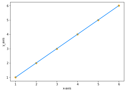
Since y equals x the equation of our line will be y=x right?  WRONG

Though,  

    y = x is mathematically the same as y = 1x, this is quite different in data science, the formula for the line will be y=1x, where 1 is the angle formed between the line and the  x-axis also known as  the slope of the line

but, 

slope = change in y / change in x = m(referred as m)

Our formula will now be y = mx.

Finally, we need to add a constant to our equation, that is a value of  y when x was zero in other words the value of  y when the line crossed the y-axis.

Finally,

our equation will be  y = mx + c (This is nothing but a model in data science)

where c is the y-intercept

Simple Linear Regression

Simple linear Regression has one dependent variable and one independent variable. Here we are trying to understand the relation between two variables for example, how a stock price changes with the change of a simple moving average.

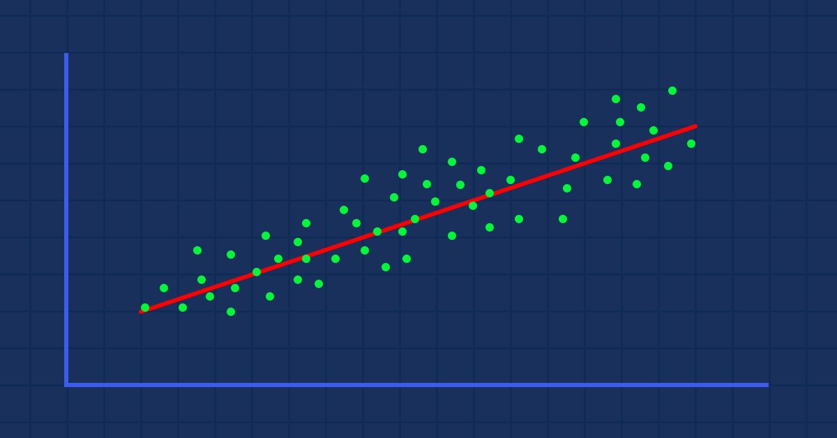
Complicated Data

Suppose we have random scattered indicator values when drawn against the stock price (something that happens in real life).

In this case, our Indicator/independent variable may not be the good predictor of our stock price/dependent variable.

The first filter that you have to apply in your datasets is to drop all columns that do not strongly correlate to your target as you are not going to build your linear model with those.

Building a linear model with non-linear related data is a huge fundamental mistake; be careful!

The relation can be inverse or reverse but it has to be strong and since we are looking for linear relationships, that is what you want to find.

So, how do we measure the strength between the independent variable and the target? We use a metric known as  the coefficient of correlation.

Coefficient of Correlation

Let's code for a script to create a dataset to be used as the main example for this article. Let's find the Predictors of NASDAQ.

input ENUM_TIMEFRAMES   timeframe = PERIOD_H1;
input int               maperiod = 50;
input int               rsiperiod = 13;

int  total_data = 744;
//+------------------------------------------------------------------+
//| Script program start function                                    |
//+------------------------------------------------------------------+
void OnStart()
  {
   string file_name = "NASDAQ_DATA.csv";
   string nasdaq_symbol = "#NQ100", s_p500_symbol ="#SP500";
   
//---
   int handle = FileOpen(file_name,FILE_CSV|FILE_READ|FILE_WRITE,",");
    if (handle == INVALID_HANDLE)
     {
      Print("data to work with is nowhere to be found Err=",GetLastError());
     }
//---
     MqlRates nasdaq[];
     ArraySetAsSeries(nasdaq,true);
     CopyRates(nasdaq_symbol,timeframe,1,total_data,nasdaq);
//---
     MqlRates s_p[];
     ArraySetAsSeries(s_p,true); 
     CopyRates(s_p500_symbol,timeframe,1,total_data,s_p);
     
//--- Moving Average Data

     int ma_handle = iMA(nasdaq_symbol,timeframe,maperiod,0,MODE_SMA,PRICE_CLOSE);
     double ma_values[];
     ArraySetAsSeries(ma_values,true);
     CopyBuffer(ma_handle,0,1,total_data,ma_values);
     
//--- Rsi values data

    int rsi_handle = iRSI(nasdaq_symbol,timeframe,rsiperiod,PRICE_CLOSE);
    double rsi_values[];
    ArraySetAsSeries(rsi_values,true);
    CopyBuffer(rsi_handle,0,1,total_data,rsi_values);

//---

     if (handle>0)
       {  
         FileWrite(handle,"S&P500","NASDAQ","50SMA","13RSI"); 
            for (int i=0; i<total_data; i++)
              {  
                string str1 = DoubleToString(s_p[i].close,Digits());
                string str2 = DoubleToString(nasdaq[i].close,Digits());
                string str3 = DoubleToString(ma_values[i],Digits());
                string str4 = DoubleToString(rsi_values[i],Digits());
                FileWrite(handle,str1,str2,str3,str4); 
              }
       }
     FileClose(handle); 
  }
//+------------------------------------------------------------------+
//|                                                                  |
//+------------------------------------------------------------------+

In the script we gathered NASDAQ closed price, 13 period RSI values, S&P 500, and 50 Period Moving Average. After a successful collection of data to a CSV file, let us visualize the data in python on anaconda's Jupyter notebook, for those who does not have anaconda installed on their machine you can run your data science python code used in this article at google colab.

Before you can open a CSV file that was created by our test script you need to convert it into UTF-8 encoding so that it could be read by python. Open the CSV file with notepad then save it encoding as UTF-8 since. It will be a good thing to copy the file in the external directory so that it will be read separately by python when you link to that directory, using pandas let's read the CSV file and store it into the data variable.

The output is as follows:

From the visual presentation of the data, we can already see that there is a very strong relationship between NASDAQ and S&P 500, and there is a strong relationship between NASDAQ and its 50 Period Moving Average. As said earlier, whenever data is scattered all over the graph the independent variable may not be a good predictor of the target when it comes to finding linear relations but let's see what the numbers speaks about their correlation and draw a conclusion on numbers rather than our eyes, to find how variables correlate to each other we will use the metric known as the correlation coefficient.

Correlation coefficient

It is used to measure the strength between the independent variable and the target.

There are several types of correlation coefficients, but we will use this most popular one for linear regression that is also known as Pearson's  correlation coefficient( R) which ranges between -1 and +1.

Correlation of extreme possible values of -1 and +1 indicates a perfect negative linear and perfect positive linear relationship respectively between x and y whereas, a correlation of 0(zero) indicates the absence of linear correlation.

The coefficient of correlation formula/Pearson's coefficient(R).

I have created a linearRegressionLib.mqh, Inside our main library, let's code the function corrcoef().

Let's start with the mean function for the values, mean is the summation of all the data then divided by their total number of elements.

double CSimpleLinearRegression::mean(double &data[])
 {
   double x_y__bar=0;
   
   for (int i=0; i<ArraySize(data); i++)
     {
      x_y__bar += data[i]; // all values summation
     }
           
    x_y__bar = x_y__bar/ArraySize(data); //total value after summation divided by total number of elements
   
   return(x_y__bar); 
 }

Now lets code for Pearson's r

double CSimpleLinearRegression::corrcoef(double &x[],double &y[])
 {
   double r=0;
   double numerator =0, denominator =0;
   double x__x =0, y__y=0;
   
   for(int i=0; i<ArraySize(x); i++)
     {
         numerator += (x[i]-mean(x))*(y[i]-mean(y));
         x__x += MathPow((x[i]-mean(x)),2);  //summation of x values minus it's mean squared 
         y__y += MathPow((y[i]-mean(y)),2);  //summation of y values minus it's mean squared   
     }
     denominator = MathSqrt(x__x)*MathSqrt(y__y);  //left x side of the equation squared times right side of the equation squared
     r = numerator/denominator;   
    return(r);
 }

when we print the result in our TestSript.mq5 

  Print("Correlation Coefficient NASDAQ vs S&P 500 = ",lr.corrcoef(s_p,y_nasdaq));
  Print("Correlation Coefficient NASDAQ vs 50SMA = ",lr.corrcoef(ma,y_nasdaq));
  Print("Correlation Coefficient NASDAQ Vs rsi = ",lr.corrcoef(rsi,y_nasdaq));

The output will be

Correlation Coefficient NASDAQ vs S&P 500 = 0.9807093773142763

Correlation Coefficient NASDAQ vs 50SMA = 0.8746579124626006

Correlation Coefficient NASDAQ Vs rsi = 0.24245225451004537

As you can see that NASDAQ and S&P500 have a very strong correlation of all other data columns (because it's correlation coefficient is very close to 1), so we have to drop other weak columns when proceeding with building our simple linear regression model.

Now we have two data columns that we are going to build our model upon let's proceed on building our model.

The Coefficient of X

The coefficient of x, also known as the slope(m), is by definition the ratio of change in Y and change in X or, in other words, the steepness of the line.

Formula:

slope = Change in Y / Change in X

Remember from Algebra, that the slope is the,  m in the formula 

Y   =   M X  +  C

To find the Linear Regression slope m the formula is

Now we have seen the formula let's code for the slope of our model.

double CSimpleLinearRegression::coefficient_of_X()
 { 
   double m=0;
   double x_mean=mean(x_values);
   double y_mean=mean(y_values);;
//---  
    {
      double x__x=0, y__y=0;
      double numerator=0, denominator=0; 
      
      for (int i=0; i<(ArraySize(x_values)+ArraySize(y_values))/2; i++)
       {
         x__x = x_values[i] - x_mean; //right side of the numerator (x-side)
         y__y = y_values[i] - y_mean; //left side of the numerator  (y-side)
        
         
         numerator += x__x * y__y;  //summation of the product two sides of the numerator
         denominator += MathPow(x__x,2); 
       }
      m = numerator/denominator;
    }
   return (m);
 }

Pay attention to the y_values and x_values arrays, These are arrays that were Initiated and copied Inside the Init() function Inside the Class CSimpleLinearRegression.

Here is the CSimpleLinearRegression::Init() function:

void CSimpleLinearRegression::Init(double& x[], double& y[])
 {
   ArrayCopy(x_values,x);
   ArrayCopy(y_values,y);
//---

   if (ArraySize(x_values)!=ArraySize(y_values))
     Print(" Two of your Arrays seems to vary In Size, This could lead to inaccurate calculations ",__FUNCTION__);
   
   int columns=0, columns_total=0;
   int rows=0;
   
   fileopen();
   while (!FileIsEnding(m_handle))
     {
        string data = FileReadString(m_handle);
          if (rows==0) 
            {
              columns_total++;
            }
         columns++;
         
        if (FileIsLineEnding(m_handle))
         {
           rows++;
           columns=0;
         }
     }
     
   m_rows = rows;
   m_columns = columns; 
   FileClose(m_handle);
//---    
 }

We've done coding the Coefficient of X now let's move to the next part.

Y-Intercept 

As said earlier the Y-intercept, is the value of y when the value of x is zero, or the value of y when the line cuts through the y-axis.

Finding the y-intercept

From the equation 

Y  =  M X  +  C

Taking MX to the left side of the equation and flipping the equation left side right, the final equation for the x-intercept will be: 

C  =  Y  -  M  X

here,

Y = mean of all y values

x = mean of all x values

Now, let's code for the function to find the y-intercept.

double CSimpleLinearRegression::y_intercept()
 {
   // c = y - mx
   return (mean(y_values)-coefficient_of_X()*mean(x_values));
 }

Were done with the y-intercept, let's build our linear regression model by printing it in our Main function LinearRegressionMain() .

void CSimpleLinearRegression::LinearRegressionMain(double &predict_y[])
 {
   double slope = coefficient_of_X();
   double constant_y_intercept= y_intercept();
   
   Print("The Linear Regression Model is "," Y =",DoubleToString(slope,2),"x+",DoubleToString(constant_y_intercept,2));
   
   ArrayResize(predict_y,ArraySize(y_values));                  
   for (int i=0; i<ArraySize(x_values); i++)
       predict_y[i] = coefficient_of_X()*x_values[i]+y_intercept();
//--- 
 }

We are also using our model to get the predicted values of y, that will be helpful, sometimes in the future when continuing to build our model and analyzing it's accuracy.

Let's call the function on the Onstart() function inside our TestScript.mq5.

lr.LinearRegressionMain(y_nasdaq_predicted);

The output will be

2022.03.03 10:41:35.888 TestScript (#SP500,H1) The Linear Regression Model is  Y =4.35241x+-4818.54986

Before we call the function in our script, it is worth explaining other parts of the library that have made this process possible. I coded a function GetDataToArray() that will be useful in the process of reading data from a specific column from a CSV file and storing that data into an array of double values.

void CSimpleLinearRegression::GetDataToArray(double &array[],string file_name,string delimiter,int column_number)
 {
   m_filename = file_name;
   m_delimiter = delimiter; 
   
   int column=0, columns_total=0;
   int rows=0;
   
   fileopen();
   while (!FileIsEnding(m_handle))
     {
        string data = FileReadString(m_handle);
          if (rows==0) 
            {
              columns_total++; 
            }
         column++;
         
       //Get data by each Column 
       
        if (column==column_number) //if we are on the specific column that we want 
          { 
            ArrayResize(array,rows+1);
            if (rows==0)
             { 
              if ((double(data))!=0) //Just in case the first line of our CSV column has a name of the column 
                 { 
                   array[rows]= NormalizeDouble((double)data,Digits());
                 }
              else { ArrayRemove(array,0,1); }
             }
            else 
              { 
               array[rows-1]= StringToDouble(data);
              }
            //Print("column ",column," "," Value ",(double)data);
          }
//---
        if (FileIsLineEnding(m_handle))
         {
           rows++;
           column=0;
         }
     }  
    FileClose(m_handle);
 }

Inside the void Function fileopen()  

void CSimpleLinearRegression::fileopen(void)
 {
   m_handle = FileOpen(m_filename,FILE_READ|FILE_WRITE|FILE_CSV,m_delimiter);      
   
   if (m_handle==INVALID_HANDLE) 
       {   
         Print("Data to work with is nowhere to be found, Error = ",GetLastError()," ", __FUNCTION__);
       }
//---
 }

Now inside our TestScript, the first thing that we have to do is to declare two arrays 

    double s_p[]; //Array for storing S&P 500 values
    double y_nasdaq[]; //Array for storing NASDAQ values

The next thing that we have to do is to pass those arrays to get their reference from our GetDataToArray() void function

    lr.GetDataToArray(s_p,file_name,",",1);
    lr.GetDataToArray(y_nasdaq,file_name,",",2);

Pay attention to the column numbers since our function arguments looks like this on the public section of our class

   void   GetDataToArray(double& array[],string filename, string delimiter, int column_number);

Make sure that you refer to right column number. As you can see how columns are arranged in our CSV file

S&P500,NASDAQ,50SMA,13RSI
4377.5,14168.6,14121.1,59.3
4351.3,14053.2,14118.1,48.0
4342.6,14079.3,14117.0,50.9
4321.2,14038.1,14115.6,46.1
4331.8,14092.9,14114.6,52.5
4336.1,14110.2,14111.8,54.7
4331.5,14101.4,14109.4,53.8
4336.4,14096.8,14104.7,53.3
.....

After calling the GetDataToArray() function, it is time to call the Init() function, as it does not make sense to initialize the library without having the data properly collected and stored into their Arrays. Calling the function in their proper order looks like this,

void OnStart()
{
    string file_name = "NASDAQ_DATA.csv";
    double s_p[];
    double y_nasdaq[];
    double y_nasdaq_predicted[];
     
    lr.GetDataToArray(s_p,file_name,",",1); //Data is taken from the first column and gets stored in the s_p Array
    lr.GetDataToArray(y_nasdaq,file_name,",",2); //Data is taken from the second column and gets stored in the y_nasdaq Array
    
//---
      lr.Init(s_p,y_nasdaq);        
        { 
         lr.LinearRegressionMain(y_nasdaq_predicted);
           
           Print("slope of a line ",lr.coefficient_of_X());
         }
}

Now that we have the predicted values stored in the array y_nasdaq_predicted Let's visualize the Dependent variable(NASDAQ), Independent variable(S&P500), and the predictions on the same curve.

Run the following code on your Jupyter notebook

The full reference of python code is attached at the end of the article.

After running successfully the above code snippet you will see the following graph

Now, we have our model and other stuff going on in our library what about the Accuracy of our model? Is our model good enough to mean anything or, to be used in anything?

To understand how good our model is at predicting the Target variable we use a Metric known as the coefficient of determinant referred to as R-squared.

R-Squared

This is the proposition of total variance of y that has been explained by the model.

To find the r-squared we need to understand the error in prediction. Error in prediction is the difference between the actual/real value of y and the predicted value of y.

mathematically,

Error = Y actual - Y predicted

The R-squared formula is 

Rsquared = 1 - (Total sum of squared errors / Total sum of squared residuals)

Why square errors?

• Errors can be positive or negative (above or below the line) we square them to keep them positive
• Negative values could decrease the error
• We also square errors to penalize large errors so that we can get the best fit possible 

R-square ranges between zero and one

Zero means the model is not able to explain any variance of y indicating that the model is the worst possible, One indicates that the model is able to explain all the variance of y in your dataset (such model doesn't exist).

You can refer to the r-squared output as the percentage of how good your model is zero means zero percent accuracy and One means One hundred percent your model is accurate.

Now let us code for the R squared.

double CSimpleLinearRegression::r_squared()
 {
   double error=0;
   double numerator =0, denominator=0;
   double y_mean = mean(y_values);
//---
  if (ArraySize(m_ypredicted)==0)
    Print("The Predicted values Array seems to have no values, Call the main Simple Linear Regression Funtion before any use of this function = ",__FUNCTION__);
  else
    {
      for (int i=0; i<ArraySize(y_values); i++)
        {
          numerator += MathPow((y_values[i]-m_ypredicted[i]),2);
          denominator += MathPow((y_values[i]-y_mean),2);
        }
      error = 1 - (numerator/denominator);
    }
   return(error);
 }

Remember that, Inside our LinearRegressionMain where we stored the predicted values in predicted_y[] array that was passed by reference, we have to copy that Array to a global variable array that was declared on the private section of our class.

    private:
                        int     m_handle;
                        string  m_filename;
                        string  m_delimiter; 
                        double  m_ypredicted[];
                        double  x_values[];
                        double  y_values[];
    

in the end of our LinearRegressionMain I added the line to copy that array to a global variable array m_ypredicted[].

//At the end of the function LinearRegressionMain(double &predict_y[]) I added the following line,

// Copy the predicted values to m_ypredicted[], to be Accessed inside the library
   ArrayCopy(m_ypredicted,predict_y);

Now let's print the R-squared value inside our TestScript 

   Print(" R_SQUARED = ",lr.r_squared());

The output will be:

2022.03.03 10:40:53.413 TestScript (#SP500,H1) R_SQUARED = 0.9590906984145334

The R-squared of our model is 0.9590 meaning that our model is able to explain more than 95% of variance in NASDAQ values, in simple words our model is more than 95% accurate in predicting the values of NASDAQ

That's it for the simple linear Regression, now let's see what a multiple linear regression would look like.

Multiple Linear Regression

Multiple linear Regression has one independent variable and more than one dependent variables.

The formula for the model of multiple linear regression is as follows

Y  =  M1X1 + M2X2 + M3X3+....+C

The y-Intercept will be only one because the line of our model will pass through the y-axis only once

This is how our library looks like after hard coding the private and public sections of our class.

class CMultipleLinearRegression: public CSimpleLinearRegression
  { 
      private:
                          int m_independent_vars;
      public:
                           CMultipleLinearRegression(void);
                          ~CMultipleLinearRegression(void);
                          
                          double coefficient_of_X(double& x_arr[],double& y_arr[]);
                          void   MultipleRegressionMain(double& predicted_y[],double& Y[],double& A[],double& B[]);
                          double y_interceptforMultiple(double& Y[],double& A[],double& B[]);
                          void   MultipleRegressionMain(double& predicted_y[],double& Y[],double& A[],double& B[],double& C[],double& D[]);
                          double y_interceptforMultiple(double& Y[],double& A[],double& B[],double& C[],double& D[]);
  };

Since we will be dealing with multiple values this is the part where we will play with a lot of reference arrays of functions Arguments,  I couldn't find the shortcut way to implement.

To create the linear Regression model for two dependent variables we will use this function.

void CMultipleLinearRegression::MultipleRegressionMain(double &predicted_y[],double &Y[],double &A[],double &B[])
 {
// Multiple regression formula =  y = M1X1+M2X2+M3X3+...+C

  double constant_y_intercept=y_interceptforMultiple(Y,A,B);
  double slope1 = coefficient_of_X(A,Y);
  double slope2 = coefficient_of_X(B,Y);
  
   Print("Multiple Regression Model is ","Y="+DoubleToString(slope1,2)+"A+"+DoubleToString(slope2,2)+"B+"+
         DoubleToString(constant_y_intercept,2));
         
   int ArrSize = (ArraySize(A)+ArraySize(B))/2;
   ArrayResize(predicted_y,ArrSize);
   for (int i=0; i<ArrSize; i++)
       predicted_y[i] = slope1*A[i]+slope2*B[i]+constant_y_intercept;
       
 }

The Y-intercept for this Instance will be based on the number of data columns that we decided to work. After deriving the formula from multiple linear regression the final formula will be:

C  =  Y  -  M1 X1 -  M2 X2

This is how it looks like after coding it

double CMultipleLinearRegression::y_interceptforMultiple(double &Y[],double &A[],double &B[])
 {
   //formula c=Y-M1X1-M2X2;
   return(mean(Y)-coefficient_of_X(A,Y)*mean(A)-coefficient_of_X(B,Y)*mean(B));
 }

In case of three variables it was just the matter of hard coding the function again and adding another variable.

void CMultipleLinearRegression::MultipleRegressionMain(double &predicted_y[],double &Y[],double &A[],double &B[],double &C[],double &D[])
 {
   double constant_y_intercept = y_interceptforMultiple(Y,A,B,C,D);
   double slope1 = coefficient_of_X(A,Y);
   double slope2 = coefficient_of_X(B,Y);
   double slope3 = coefficient_of_X(C,Y);
   double slope4 = coefficient_of_X(D,Y);
//---
   Print("Multiple Regression Model is ","Y="+DoubleToString(slope1,2),"A+"+DoubleToString(slope2,2)+"B+"+
         DoubleToString(slope3,2)+"C"+DoubleToString(slope4,2)+"D"+DoubleToString(constant_y_intercept,2));
//---
   int ArrSize = (ArraySize(A)+ArraySize(B))/2;
   ArrayResize(predicted_y,ArrSize);
   for (int i=0; i<ArrSize; i++)
       predicted_y[i] = slope1*A[i]+slope2*B[i]+slope3*C[i]+slope4*D[i]+constant_y_intercept;
 }

The Constant/Y-intercept for our multiple linear regression was as said earlier that it is going to be.

double CMultipleLinearRegression::y_interceptforMultiple(double &Y[],double &A[],double &B[],double &C[],double &D[])
 {
   return (mean(Y)-coefficient_of_X(A,Y)*mean(A)-coefficient_of_X(B,Y)*mean(B)-coefficient_of_X(C,Y)*mean(C)-coefficient_of_X(D,Y)*mean(D));
 }

Linear Regression Assumptions

The Linear Regression model is based on a set of assumptions, if the underlying dataset does not meet these assumptions then data may have to be transformed or a linear model may not be a good fit.

• Assumption of linearity, Assumes a linear relationship between the dependent/target variable and the independent/predictor variables
• Assumption of normality of the error distribution

1. The errors should be normally distributed along with the model
2. A scatter plot between the actual values and the predicted values should show the data distributed equally across the model

Advantages of a Linear Regression Model

Simple to implement and easier to interpret the outputs and the coefficients.

Disadvantages

1. Assumes a linear relationship between dependent and independent variables, that is it assumes there is a straight-line relationship between them
2. Outliers have a huge effect on the regression
3. Linear Regression assumes independence between the attributes 
4. Linear Regression looks at a relationship between the mean of the dependent variable and the independent variable 
5. Just as the mean is not a complete description of a single variable, linear regression is not a complete description of relationships among variables 
6. Boundaries are linear

Final Thoughts

I think linear regression algorithms can be very useful when creating trading strategies based on correlation of pairs and other stuff like indicators, though our library Is nowhere near a finished library I have not included the training and testing of our model and further improvements of the results, that part will be on the next article, stay tuned I have python code linked on my Github repository here any contribution to the library will be appreciated, also feel free to share your thought on the discussion section of the article.

See you soon