Data Science and Machine Learning (Part 02): Logistic Regression

Unlike Linear Regression that we discussed in part 01, Logistic Regression is a classification method based on linear regression.
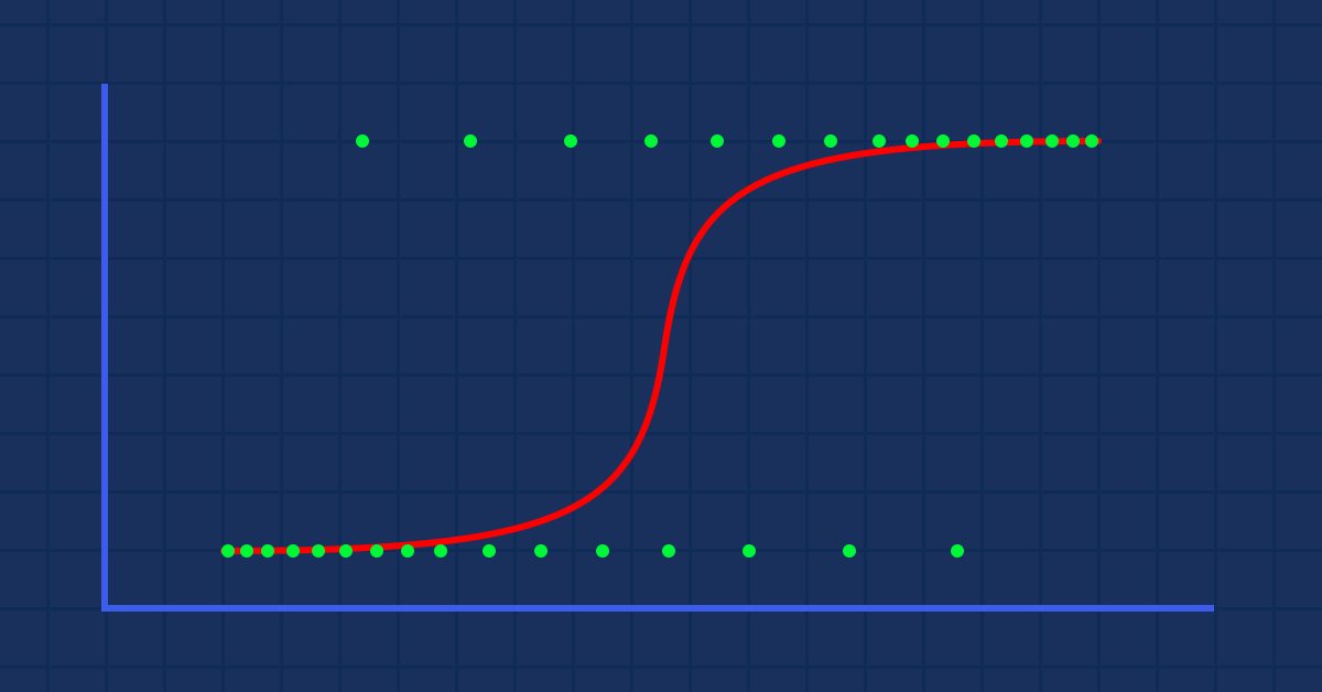
Theory: Suppose that we draw a graph of the probability of someone being obese versus their weight.
In this case, we can't use a linear model, we'll use another technique to transform this line into an S-curve known as Sigmoid.
Since Logistic Regression produces results in a binary format which is used to predict the outcome of the categorical dependent variable so the outcome should be discrete/categorical such as:
- 0 or 1
- Yes or No
- True or False
- High or Low
- Buy or Sell
In our library that we are going to create, we are going to ignore other discrete values. Our focus will be on the binary-only (0,1).
Since our values of y are supposed to be between 0 and 1, our line has to be clipped at 0 and 1. This can be achieved through the formula:

Which will give us this graph

The Linear model is passed to a logistic function (sigmoid/p) =1/1+e^t where t is the linear model the result which is values between 0 and 1. This represents the probability of a data point belonging to a class.
Instead of using y of a linear model as a dependent, its function is shown as " p" is used as dependent
p = 1/1+e^-(c+m1x1+m2x2+....+mnxn) ,case of multiple values
As said earlier, the sigmoid curve aims to convert infinity values into binary format output(0 or 1). But what if I have a data point located at 0.8, how can one decide that the value is zero or one? This is where the threshold values come into play.

The threshold indicates the probability of either winning or losing, it is located at 0.5 (center of 0 and 1).
Any value greater than or equal to 0.5 will be rounded to one, hence regarded as a winner, whilst any value below 0.5 will be rounded to 0 hence regarded as a loser at this point, it is time that we see the difference between linear and logistic regression.
Linear Vs Logistic Regression
| Linear | Logistic Regression |
|---|---|
| Continuous variable | Categorical variable |
| Solves regression Problems | Solves classifications problems |
| Model has a straight equation | Model has a logistic equation |
Before we dive into the coding part and the algorithms to classify the data, several steps could help us understand the data and make it easier for us to build our model:
- Collecting & Analyzing Data
- Cleaning your Data
- Checking the Accuracy
01:Collecting & Analyzing Data
In this section, we are going to write a lot of python code to visualize our data. Let's start by importing the libraries that we are going to use to extract and visualize the data in the Jupyter notebook.
For the sake of building our library, we are going to use the titanic data, for those who are not familiar with it, it is the data about the titanic ship accident which sank in the North Atlantic Ocean on 15 April 1912 after striking an iceberg, Wikipedia. All the python codes and the dataset can be found on my GitHub linked at the end of the Article.

The columns stands for
survival - Survival (0 = No; 1 = Yes)
class - Passenger Class (1 = 1st; 2 = 2nd; 3 = 3rd)
name - Name
sex - Sex
age - Age
sibsp - Number of Siblings/Spouses Aboard
parch - Number of Parents/Children Aboard
ticket - Ticket Number
fare - Passenger Fare
cabin - Cabin
embarked - Port of Embarkation (C = Cherbourg; Q = Queenstown; S = Southampton)
Now that we have our data collected and stored the data to a variable titanic_data let's start visualizing data in columns, starting with survival column.
sns.countplot(x="Survived", data = titanic_data)
output

This tells us that the minority of passengers survived the accident about half of the passengers that were on the ship survived the accident.
Let's visualize the survival number according to sex
sns.countplot(x='Survived', hue='Sex', data=titanic_data)

I don't know what happened to the males that day, but the females survived more than twice the number of males
Let's visualize the survival number according to class groups
sns.countplot(x='Survived', hue='Pclass', data=titanic_data)

Let's plot the histogram of the passengers age groups that were in the ship, here we can't use the Count-plots to visualize our data since there are many different values of age on our dataset that are not organized.
titanic_data['Age'].plot.hist()Output:

Lastly, let's visualize the histogram of the fare in the ship
titanic_data['Fare'].plot.hist(bins=30, figsize=(10,10))

That's it for visualizing the data though we have visualized only 5 columns out of 12 because I think those are important columns, let's now clean our data.
02: Cleaning our Data
Here we clean our data by removing the NaN (missing) values while avoiding/removing unnecessary columns in the dataset.
Using logistic regression you need to have double and integer values so you have to avoid non-meaningful string values in this case we will ignore the following columns:
- Name column (it has no meaningful information)
- Ticket column (doesn't make any sense to the survival of the accident)
- Cabin column (it has too many missing values, even the first 5 rows show that)
- Embarked(I think it is irrelevant)
To do so I will open the CSV file in WPS office and manually remove the columns, you can use any spreadsheet program of your choice.
After removing the columns using a spreadsheet let's visualize the new data.
new_data = pd.read_csv(r'C:\Users\Omega Joctan\AppData\Roaming\MetaQuotes\Terminal\892B47EBC091D6EF95E3961284A76097\MQL5\Files\titanic.csv')
new_data.head(5)
Output:

We now have cleaned data though we still have missing values in the age column not to mention we have the string values in the sex column. Let's fix the issue through some code. Let's create a label encoder to convert the string male and female into 0 and 1 respectively.
void CLogisticRegression::LabelEncoder(string &src[],int &EncodeTo[],string members="male,female")
 {
   string MembersArray[];
   ushort separator = StringGetCharacter(m_delimiter,0);
   StringSplit(members,separator,MembersArray); //convert members list to an array
   ArrayResize(EncodeTo,ArraySize(src)); //make the EncodeTo array same size as the source array

      int binary=0;
      for(int i=0;i<ArraySize(MembersArray);i++) // loop the members array
        {
           string val = MembersArray[i];
           binary = i; //binary to assign to a member
           int label_counter = 0;

           for (int j=0; j<ArraySize(src); j++)
              {
                string source_val = src[j];
                 if (val == source_val)
                   {
                    EncodeTo[j] = binary;
                    label_counter++;
                   }
              }
           Print(MembersArray[binary]," total =",label_counter," Encoded To = ",binary);
        }
 }
To get the source Array named as src[] I also programmed a function to obtain data from a specific column in a CSV file then put it into an array of string values MembersArray[], check it out:
void CLogisticRegression::GetDatatoArray(int from_column_number, string &toArr[])
 {

   int handle  = FileOpen(m_filename,FILE_READ|FILE_WRITE|FILE_CSV|FILE_ANSI,m_delimiter);
   int counter=0;

   if (handle == INVALID_HANDLE)
      Print(__FUNCTION__," Invalid csv handle err=",GetLastError());

    else
     {
       int column = 0, rows=0;
       while (!FileIsEnding(handle))
         {
           string data = FileReadString(handle);

           column++;
//---
           if (column==from_column_number) //if column in the loop is the same as the desired column
              {
                  if (rows>=1) //Avoid the first column which contains the column's header
                    {
                        counter++;
                        ArrayResize(toArr,counter);
                        toArr[counter-1]=data;
                    }

              }
//---
           if (FileIsLineEnding(handle))
             {
               rows++;
               column=0;
             }
         }
     }
   FileClose(handle);
 }
Inside our testscript.mq5, this is how to properly call the functions and to Initialize the Library:
#include "LogisticRegressionLib.mqh";
CLogisticRegression Logreg;
//+------------------------------------------------------------------+
//| Script program start function                                    |
//+------------------------------------------------------------------+
void OnStart()
  {
//---
    Logreg.Init("titanic.csv",",");


    string Sex[];
    int SexEncoded[];
    Logreg.GetDatatoArray(4,Sex);
    Logreg.LabelEncoder(Sex,SexEncoded,"male,female");

    ArrayPrint(SexEncoded);
  }
Output printed out, after successfully running the script,
male total =577 Encoded To = 0
female total =314 Encoded To = 1
[ 0] 0 1 1 1 0 0 0 0 1 1 1 1 0 0 1 1 0 0 1 1 0 0 1 0 1 1 0 0 1 0 0 1 1 0 0 0 0 0 1 1 1 1 0 1 1 0 0 1 0 1 0 0 1 1 0 0 1 0 1 0 0 1 0 0 0 0 1 0 1 0 0 1 0 0 0
[ 75] 0 0 0 0 1 0 0 1 0 1 1 0 0 1 0 0 0 0 0 0 0 0 0 1 0 1 0 0 0 0 0 1 0 0 1 0 1 0 1 1 0 0 0 0 1 0 0 0 1 0 0 0 0 1 0 0 0 1 1 0 0 1 0 0 0 1 1 1 0 0 0 0 1 0 0
... ... ... ...
... ... ... ...
[750] 1 0 0 0 1 0 0 0 0 1 0 0 0 1 0 1 0 1 0 0 0 0 1 0 1 0 0 1 0 1 1 1 0 0 0 0 1 0 0 0 0 0 1 0 0 0 1 1 0 1 0 1 0 0 0 0 0 1 0 1 0 0 0 1 0 0 1 0 0 0 1 0 0 1 0
[825] 0 0 0 0 1 1 0 0 0 0 1 0 0 0 0 0 0 1 0 0 0 0 0 0 1 0 0 1 1 1 1 1 0 1 0 0 0 1 1 0 1 1 0 0 0 0 1 0 0 1 1 0 0 0 1 1 0 1 0 0 1 0 1 1 0 0
Before your encode your values pay attention to the members="male,female" on your function argument, the first value to appear on your string will be encoded as 0, as you can see on the male column appears first thus all male will be encoded to 0 the females will be encoded to 1. This function is not restricted to two values though, you can encode as much as you want as long as the string makes some sense to your data.
Missing Values
If you pay attention to the Age column you will notice that there are missing values, the missing values may be mainly due to one reason... death, in our dataset, making it impossible to identify the Age of an individual, you can identify those gaps by looking at the dataset thought that may be time consuming especially on large datasets, since we are also using pandas to visualize our data let's find out the missing rows in all the columns
titanic_data.isnull().sum()
The output will be:
PassengerId 0
Survived 0
Pclass 0
Sex 0
Age 177
SibSp 0
Parch 0
Fare 0
dtype: int64
Out of 891, 177 rows in our Age column have missing values (NAN).
Now, we are going to replace the missing values in our column by replacing the values with the mean of all the values.
void CLogisticRegression::FixMissingValues(double &Arr[])
 {
   int counter=0; double mean=0, total=0;
   for (int i=0; i<ArraySize(Arr); i++) //first step is to find the mean of the non zero values
       {
         if (Arr[i]!=0)
           {
             counter++;
             total += Arr[i];
           }
       }
     mean = total/counter; //all the values divided by their total number
     Print("mean ",MathRound(mean)," before Arr");
     ArrayPrint(Arr);

     for (int i=0; i<ArraySize(Arr); i++)
       {
         if (Arr[i]==0)
           {
             Arr[i] = MathRound(mean); //replace zero values in array
           }
       }
     Print("After Arr");
     ArrayPrint(Arr);
 }
This function finds the mean of all the non zero values then it substitutes all the zero's values in array with the mean value.
The output after successfully running the function, As you can see all zero values have been replaced with 30.0 which was the mean age of the passengers in the titanic.
mean 30.0 before Arr
[ 0] 22.0 38.0 26.0 35.0 35.0 0.0 54.0 2.0 27.0 14.0 4.0 58.0 20.0 39.0 14.0 55.0 2.0 0.0 31.0 0.0 35.0 34.0 15.0 28.0 8.0 38.0 0.0 19.0 0.0 0.0
… … … … … … … … …
[840] 20.0 16.0 30.0 34.5 17.0 42.0 0.0 35.0 28.0 0.0 4.0 74.0 9.0 16.0 44.0 18.0 45.0 51.0 24.0 0.0 41.0 21.0 48.0 0.0 24.0 42.0 27.0 31.0 0.0 4.0
[870] 26.0 47.0 33.0 47.0 28.0 15.0 20.0 19.0 0.0 56.0 25.0 33.0 22.0 28.0 25.0 39.0 27.0 19.0 0.0 26.0 32.0
After Arr
[ 0] 22.0 38.0 26.0 35.0 35.0 30.0 54.0 2.0 27.0 14.0 4.0 58.0 20.0 39.0 14.0 55.0 2.0 30.0 31.0 30.0 35.0 34.0 15.0 28.0 8.0 38.0 30.0 19.0 30.0 30.0
… … … … … … … … …
[840] 20.0 16.0 30.0 34.5 17.0 42.0 30.0 35.0 28.0 30.0 4.0 74.0 9.0 16.0 44.0 18.0 45.0 51.0 24.0 30.0 41.0 21.0 48.0 30.0 24.0 42.0 27.0 31.0 30.0 4.0
[870] 26.0 47.0 33.0 47.0 28.0 15.0 20.0 19.0 30.0 56.0 25.0 33.0 22.0 28.0 25.0 39.0 27.0 19.0 30.0 26.0 32.0
Building The Logistic Regression Model
First, let's build our logistic regression where we will have one independent variable and one dependent variable. Then we will scale up to a full solution model to our problem later on.
Let's build the model on two variables Survived Versus Age, let's find out what was the chances that a person could survive based on their Age.
So far, we know that deep inside a logistic model there is a linear model in it. Let's start by coding the functions that make a linear model possible.
Coefficient_of_X() and y_intercept() these functions are not new, we build them on the first article of this series, consider reading it for more information on these functions and linear regression at large.
double CLogisticRegression::y_intercept()
 {
   // c = y - mx
   return (y_mean-coefficient_of_X()*x_mean);
 }
//+------------------------------------------------------------------+
//|                                                                  |
//+------------------------------------------------------------------+
double CLogisticRegression::coefficient_of_X()
 {
   double m=0;
//---
    {
      double x__x=0, y__y=0;
      double numerator=0, denominator=0;

      for (int i=0; i<ArraySize(m_xvalues); i++)
       {
         x__x = m_xvalues[i] - x_mean; //right side of the numerator (x-side)
         y__y = m_yvalues[i] - y_mean; //left side of the numerator  (y-side)


         numerator += x__x * y__y;  //summation of the product two sides of the numerator
         denominator += MathPow(x__x,2);
       }
      m = numerator/denominator;
    }
   return (m);
 }
Now, let's program the logistic model from the formula.

Note that z is also referred to as the log-odds because the inverse of the sigmoid states that z can be defined as the log of the probability of the 1 label (e.g., "Survived") divided by the probability of the 0 label (e.g., "did not survive"):

In this case y = mx+c (remember from linear model).
Turning this into code the outcome will be,
     double y_= (m*m_xvalues[i])+c;
     double z = log(y_)-log(1-y_); //log loss

     p_hat = 1.0/(MathPow(e,-z)+1);
Pay attention to what has been done here on the z value the formula is log(y/1-y), but the code is written as log(y_)-log(1-y_); Remember from the Laws of Logarithms in math!! The division of logarithms with the same base results to the subtraction of the exponents, read.
This is basically our model when the formula is programmed, but there is a lot going on inside our LogisticRegression() function, here is all that is inside the function:
double CLogisticRegression::LogisticRegression(double &x[],double &y[],int& Predicted[],double train_size_split = 0.7)
 {

   int arrsize = ArraySize(x); //the input array size
   double p_hat =0; //store the probability

//---

   int train_size = (int)MathCeil(arrsize*train_size_split);
   int test_size = (int)MathFloor(arrsize*(1-train_size_split));

   ArrayCopy(m_xvalues,x,0,0,train_size);
   ArrayCopy(m_yvalues,y,0,0,train_size);

//---

   y_mean = mean(m_yvalues);
   x_mean = mean(m_xvalues);

//   Training our model in the background

   double c = y_intercept(), m = coefficient_of_X();


//--- Here comes the logistic regression model

      int TrainPredicted[];
      double sigmoid = 0;

      ArrayResize(TrainPredicted,train_size); //resize the array to match the train size
      Print("Training starting..., train size=",train_size);

      for (int i=0; i<train_size; i++)
        {
          double y_= (m*m_xvalues[i])+c;
          double z = log(y_)-log(1-y_); //log loss

          p_hat = 1.0/(MathPow(e,-z)+1);

          double odds_ratio = p_hat/(1-p_hat);

          TrainPredicted[i] = (int) round(p_hat); //round the values to give us the actual 0 or 1

          if (m_debug)
           PrintFormat("%d Age =%.2f survival_Predicted =%d ",i,m_xvalues[i],TrainPredicted[i]);
        }

//--- Testing our model
   if (train_size_split<1.0) //if there is room for testing
      {

         ArrayRemove(m_xvalues,0,train_size); //clear our array
         ArrayRemove(m_yvalues,0,train_size); //clear our array from train data

         ArrayCopy(m_xvalues,x,0,train_size,test_size); //new values of x, starts from where the training ended
         ArrayCopy(m_yvalues,y,0,train_size,test_size);  //new values of y, starts from where the testing ended

         Print("start testing...., test size=",test_size);
         ArrayResize(Predicted,test_size); //resize the array to match the test size

         for (int i=0; i<test_size; i++)
           {
             double y_= (m*m_xvalues[i])+c;
             double z = log(y_)-log(1-y_); //log loss

             p_hat = 1.0/(MathPow(e,-z)+1);

             double odds_ratio = p_hat/(1-p_hat);

             TrainPredicted[i] = (int) round(p_hat); //round the values to give us the actual 0 or 1

             if (m_debug)
               PrintFormat("%d Age =%.2f survival_Predicted =%d , Original survival=%.1f ",i,m_xvalues[i],Predicted[i],m_yvalues[i]);
           }
      }
Now, let's train and test our model in our TestScript.mq5
    double Age[];
    Logreg.GetDatatoArray(5,Age);
    Logreg.FixMissingValues(Age);

    double y_survival[];
    int Predicted[];
    Logreg.GetDatatoArray(2,y_survival);
    Logreg.LogisticRegression(Age,y_survival,Predicted);
The output of a successful script run will be:
Training starting..., train size=624
0 Age =22.00 survival_Predicted =0
1 Age =38.00 survival_Predicted =0
... .... ....
622 Age =20.00 survival_Predicted =0
623 Age =21.00 survival_Predicted =0
start testing...., test size=267
0 Age =21.00 survival_Predicted =0
1 Age =61.00 survival_Predicted =1
.... .... ....
265 Age =26.00 survival_Predicted =0
266 Age =32.00 survival_Predicted =0
Great. Our model is now working and we can at least obtain the results from it, but is the model making good predictions?
We need to check its accuracy.
The Confusion Matrix

As we all know, every good or bad model can make predictions, I have created a CSV file for the predictions that our model has made sided with the original values from testing data on survival of passengers, again 1 means survived, 0 means did not survive.
Here are just a few 10 columns:
| Original | Predicted | |
|---|---|---|
| 0 | 0 | 0 |
| 1 | 0 | 1 |
| 2 | 0 | 1 |
| 3 | 1 | 0 |
| 4 | 0 | 0 |
| 5 | 0 | 0 |
| 6 | 1 | 1 |
| 7 | 0 | 1 |
| 8 | 1 | 0 |
| 9 | 0 | 0 |
We calculate the confusion matrix using:
- TP - True Positive
- TN - True Negative
- FP - False Positive
- FN - False Negative
Now, what are these values?
TP( True Positive )
Is when the Original value is Positive (1), and your model also predicts Positive (1)
TN( True Negative )
Is when the Original value is Negative (0), and your model also predicts Negative (0)
FP( False Positive )
Is when the original value is Negative (0), but your model predicts a positive (1)
FN ( False Negative )
Is when the original value is Positive (1), but your model predicts a negative (0)
Now that you know the values let's calculate the confusion matrix for the above sample as an Example
| Original | Predicted | TP/TN/FP/FN | |
|---|---|---|---|
| 0 | 0 | 0 | TN |
| 1 | 0 | 1 | FP |
| 2 | 0 | 1 | FP |
| 3 | 1 | 0 | FN |
| 4 | 0 | 0 | TN |
| 5 | 0 | 0 | TN |
| 6 | 1 | 1 | TP |
| 7 | 0 | 1 | FP |
| 8 | 1 | 0 | FN |
| 9 | 0 | 0 | TN |
The confusion Matrix can be used to calculate Accuracy of our model using this formula.
From our table:
- TN = 4
- TP = 1
- FN = 2
- FP = 3

Accuracy = 1 + 5 / 4 + 1 + 2 + 3
Accuracy = 0.5
In this case our accuracy is 50% .( 0.5*100% converting it to percentage)
Now, that you understand how 1X1 confusion matrix works. It time to convert it into code and analyze the Accuracy of our model on the entire Dataset
void CLogisticRegression::ConfusionMatrix(double &y[], int &Predicted_y[], double& accuracy)
 {
    int TP=0, TN=0,  FP=0, FN=0;

    for (int i=0; i<ArraySize(y); i++)
       {
         if ((int)y[i]==Predicted_y[i] && Predicted_y[i]==1)
            TP++;
         if ((int)y[i]==Predicted_y[i] && Predicted_y[i]==0)
            TN++;
         if (Predicted_y[i]==1 && (int)y[i]==0)
            FP++;
         if (Predicted_y[i]==0 && (int)y[i]==1)
            FN++;
       }
     Print("Confusion Matrix \n ","[ ",TN,"  ",FP," ]","\n","  [  ",FN,"  ",TP,"  ] ");
     accuracy = (double)(TN+TP) / (double)(TP+TN+FP+FN);
 }
Now let's go back to our Main Function in our class known as LogisticRegression(), this time we are going to turn it into a double function that returns the accuracy of the model, I am also going to reduce the number of Print() methods but add them to an if-statement as we don't want to print the values every time unless we want to debug our class. All the changes are highlighted in blue:
double CLogisticRegression::LogisticRegression(double &x[],double &y[],int& Predicted[],double train_size_split = 0.7)
 {

   double accuracy =0; //Accuracy of our Train/Testmodel
   int arrsize = ArraySize(x); //the input array size
   double p_hat =0; //store the probability

//---

   int train_size = (int)MathCeil(arrsize*train_size_split);
   int test_size = (int)MathFloor(arrsize*(1-train_size_split));

   ArrayCopy(m_xvalues,x,0,0,train_size);
   ArrayCopy(m_yvalues,y,0,0,train_size);

//---

   y_mean = mean(m_yvalues);
   x_mean = mean(m_xvalues);

//   Training our model in the background

   double c = y_intercept(), m = coefficient_of_X();


//--- Here comes the logistic regression model

      int TrainPredicted[];
      double sigmoid = 0;

      ArrayResize(TrainPredicted,train_size); //resize the array to match the train size
      Print("Training starting..., train size=",train_size);

      for (int i=0; i<train_size; i++)
        {
          double y_= (m*m_xvalues[i])+c;
          double z = log(y_)-log(1-y_); //log loss

          p_hat = 1.0/(MathPow(e,-z)+1);

          TrainPredicted[i] = (int) round(p_hat); //round the values to give us the actual 0 or 1

          if (m_debug)
           PrintFormat("%d Age =%.2f survival_Predicted =%d ",i,m_xvalues[i],TrainPredicted[i]);
        }
      ConfusionMatrix(m_yvalues,TrainPredicted,accuracy); //be careful not to confuse the train predict values arrays
      printf("Train Model Accuracy =%.5f",accuracy);

//--- Testing our model
   if (train_size_split<1.0) //if there is room for testing
      {

         ArrayRemove(m_xvalues,0,train_size); //clear our array
         ArrayRemove(m_yvalues,0,train_size); //clear our array from train data

         ArrayCopy(m_xvalues,x,0,train_size,test_size); //new values of x, starts from where the training ended
         ArrayCopy(m_yvalues,y,0,train_size,test_size);  //new values of y, starts from where the testing ended

         Print("start testing...., test size=",test_size);
         ArrayResize(Predicted,test_size); //resize the array to match the test size

         for (int i=0; i<test_size; i++)
           {
             double y_= (m*m_xvalues[i])+c;
             double z = log(y_)-log(1-y_); //log loss

             p_hat = 1.0/(MathPow(e,-z)+1);

             TrainPredicted[i] = (int) round(p_hat); //round the values to give us the actual 0 or 1

             if (m_debug)
               PrintFormat("%d Age =%.2f survival_Predicted =%d , Original survival=%.1f ",i,m_xvalues[i],Predicted[i],m_yvalues[i]);
           }
        ConfusionMatrix(m_yvalues,Predicted,accuracy);
        printf("Testing Model Accuracy =%.5f",accuracy);
      }

    return (accuracy); //Lastly, the testing Accuracy will be returned
 }
Successfully script run will output the following:
Training starting..., train size=624
Confusion Matrix
[ 378 0 ]
[ 246 0 ]
Train Model Accuracy =0.60577
start testing...., test size=267
Confusion Matrix
[ 171 0 ]
[ 96 0 ]
Testing Model Accuracy =0.64045
Hooray! We are now able to identify how good our model is through numbers, though the Accuracy of 64.045% on the testing data is not good enough to use the model in making predictions (in my opinions) at least for now, we have a library that could help us classify the data using logistic regression.
Further, explanations on the main function:
double CLogisticRegression::LogisticRegression(double &x[],double &y[],int& Predicted[],double train_size_split = 0.7)
The input train_size_split is for splitting the data into training and testing by default the split is 0.7 which is means 70% percent of the data will be for training while the remaining 30% will be for testing purposes, the Predicted[] reference array will return the testing predicted data.
Binary Cross Entropy aka Loss Function
Just like mean Squared Error is the error function for linear regression, Binary cross-entropy is the cost function for logistic regression.
Theory:
Let's see how it works in two use cases for logistic regression i.e: when the actual output is 0 & 1
01: When the actual output value is 1
Consider the model for two input samples p1 = 0.4 and p2 = 0.6. It is expected that p1 should be penalized more than p2 because it is far away from 1 compared to p1.
From a mathematical point of view, the negative logarithm of a small number is a large number and vice versa.
To penalize the inputs we will use the formula
penalty = -log(p)
In these two cases
- Penalty = -log(0.4)=0.4 i.e. the penalty on p1 is 0.4
- Penalty = -log(0.6)=0.2 i.e. the penalty on p2 is 0.2
02: When the actual output value is 0
Consider the model output for two input samples, p1 = 0.4 and p2= 0.6 (same as in the previous case). It is expected that p2 should be penalized more than p1 because it is far from 0 but, keep in mind that the output of the logistic model is the probability of a sample being positive, To penalize the input probabilities we need to find the probability of a sample being negative, that's easy here is the formula
Probability of sample being negative = 1-probability of a sample being positive
So, to find the penalty in this case the formula for penalty will be
penalty = -log(1-p)
In these two cases
- penalty = -log(1-p) = -log(1-0.4) =0.2 i.e. the penalty is 0.2
- penalty = -log(1-p) = -log(1-0.6) =0.4 i.e. the penalty is 0.4
The penalty on p2 is greater than on p1 (works as expected) cool!
Now the penalty for a single input sample whose model output is p and the true output value is y can be calculated as follows.
if input sample is positive y=1:
penalty = -log(p)
else:
penalty = -log(1-p)
A single line equation equivalent to the above if-else block statement can be written as
penalty = -( y*log(p) + (1-y)*log(1-p) )
where
y = actual values in our dataset
p = raw predicted probability of the model(before roundoff)
Let's prove that this equation is equivalent to the above if-else statement
01: when the output values y = 1
penalty = -( 1*log(p) + (1-1)*log(1-p) ) = -log(p) hence proven
02: when the output value y = 0
penalty = -( 0*log(p) + (1-0)* log(1-p) ) = log(1-p) hence proven
Finally, the log loss function for N input samples looks like

Log-loss is indicative of how close the prediction probability is to the corresponding actual/true value (0 or 1 in the case of binary classification). The more the predicted probability diverges from the actual value, the higher is the log-loss value.
Cost functions such as log-loss and many others can be used as a metric on how good the model is but the biggest use is when optimizing the model for the best parameters using gradient descent or other optimizing algorithms(we will discuss in later series stay tuned).
If you can measure it, you can improve it. That's the main purpose of the cost functions.
from our testing and training dataset it appears that our log-loss lies between 0.64 - 0.68 which is not ideal(roughly speaking).
training dataset
Logloss =0.6858006105398738
testing dataset
Logloss =0.6599503403665642
Here is how we can convert our log-loss function into code
double CLogisticRegression::LogLoss(double &rawpredicted[])
 {
   double log_loss =0;
   double penalty=0;
   for (int i=0; i<ArraySize(rawpredicted); i++ )
      {
        penalty += -((m_yvalues[i]*log(rawpredicted[i])) + (1-m_yvalues[i]) * log(1-rawpredicted[i])); //sum all the penalties

         if (m_debug)
            printf("penalty =%.5f",penalty);
      }
    log_loss = penalty/ArraySize(rawpredicted); //all the penalties divided by their total number
    Print("Logloss =",log_loss);

    return(log_loss);
 }
To get the raw predicted output, we need to go back to the main testing and training for loops and store the data into the raw predicted array right before the process of rounding off the probabilities.
Multiple Dynamic Logistic Regression Challenge
The biggest challenge I faced when building both linear and logistic regression libraries in both articles this and the previous one is multiple dynamic regression functions where we could use them for multiple data columns without having to hard-code things up for every data that gets added to our model, in the previous Article I hardcoded two functions with the same name the only difference between them was the number of data each model could work with, one was able to work with two independent variables the other with four respectively:
void   MultipleRegressionMain(double& predicted_y[],double& Y[],double& A[],double& B[]);
void   MultipleRegressionMain(double& predicted_y[],double& Y[],double& A[],double& B[],double& C[],double& D[]);
But, this method is inconvenient and it feels like a premature way of coding things up and it violates the rules of clean code and DRY (don't repeat yourself principles that OOP is trying to help us achieve).
Unlike python with flexible functions that could take a large number of functional arguments with the help of *args and **kwargs, In MQL5 this could be achieved using string only as far as I can think, I believe this is our starting point.
void CMultipleLogisticRegression::MLRInit(string x_columns="3,4,5,6,7,8")
The input x_columns represents all the independent variables columns that we will use in our library, these columns will require us to have multiple independent arrays for each of the columns but, there is no way we can create arrays dynamically, so the use of arrays fall flat here.
We can create multiple CSV files dynamically and use them as arrays, for sure but this will make our programs more expensive when it comes to the use of computer resources compared to the use of arrays, especially when dealing with multiple data not to mention the while loops that we will frequently use to open the files will slow the whole process down, I'm not 100% sure so correct me if I'm wrong.
Though we can still use the mentioned way.
I have discovered the way forward to use arrays we are going to store all the data from all the columns in one array then use the data separately from one that single Array.
   int start = 0;
   if (m_debug) //if we are on debug mode print Each Array vs its row
      for (int i=0; i<x_columns_total; i++)
         {
            ArrayCopy(EachXDataArray,m_AllDataArray,0,start,rows_total);
            start += rows_total;

            Print("Array Number =",i," From column number ",m_XColsArray[i]);
            ArrayPrint(EachXDataArray);
         }
Inside the for loop, we can manipulate the data in the arrays and perform all the calculations for the model the way want for all the columns, I have tried this method but I'm still on the unsuccessful attempt, the reason I explained this hypothesis is to let everyone reading this article understand this challenge and I welcome all your opinions in the comment sections on how we can code this multiple dynamic logistic regression function my full attempt to creating this library is found on this link https://www.mql5.com/en/code/38894.
This attempt has been unsuccessful but it has hopes and I believe it is worth sharing.
Advantages of Logistic Regression
- Does not assume regarding the distribution of class in feature space
- Easily extended to multiple classes(multinomial regression)
- Natural probabilistic view of class predictions
- Quick to train
- very fast in classifying unknown records
- Good accuracy for many simple datasets
- Resistant to overfitting
- Can interpret model coefficients as an indicator of feature importance
Disadvantages
- Constructs linear boundaries
Final Thoughts
That's all for this article, Logistic regression is used in multiple fields in real life such as classifying emails as spam and not spam, detecting handwriting, and much more interesting stuff.
I know we are not going to use logistic regression algorithms to classify titanic data or any of the mentioned fields though, especially in the MetaTrader 5 platform, as said earlier, the dataset was used just for the sake of building the library in comparison with the output that was achieved in python linked here > https://github.com/MegaJoctan/LogisticRegression-MQL5-and-python. In the next article, we are going to see how we can use the logistic models to predict the stock market crash.
Since this Article has become too long I leave the multiple regression task as homework to all the readers.
Warning: All rights to these materials are reserved by MetaQuotes Ltd. Copying or reprinting of these materials in whole or in part is prohibited.
This article was written by a user of the site and reflects their personal views. MetaQuotes Ltd is not responsible for the accuracy of the information presented, nor for any consequences resulting from the use of the solutions, strategies or recommendations described.


 Multiple indicators on one chart (Part 01): Understanding the concepts
 Learn how to design a trading system by CCI
 Learn how to design a trading system by MACD
 Mathematics in trading: Sharpe and Sortino ratios
- Free trading apps
- Over 8,000 signals for copying
- Economic news for exploring financial markets
You agree to website policy and terms of use