
Data Science and Machine Learning — Neural Network (Part 01): Feed Forward Neural Network demystified
“...weary of knowing too much and understanding too little.”
― Jan Karon, Home to Holly Springs
Introduction
Neural networks sound like this fancy new thing that seems as a way forward to build holy grails trading systems, many traders are stunned by the programs made of neural networks, as they seem to be good at predicting market movements basically, they are good at any task at hand. I too believe they have tremendous potential when it comes to predicting or classifying based on the untrained/never seen data.
As good as they might they need to be constructed by someone who is knowledgeable and sometimes need to be optimized to make sure that not only the Multilayer perceptron is in the correct architecture but also the type of problem is the one that needs neural network rather than just a linear or a logistic regression model or, any other machine learning technique.
Neural Networks, are a broader subject, and so is Machine learning, in general, that's why I decided to add a sub header for neural networks as I will proceed with other aspects of ML in the other subheading in the series.
In this article, we are going to see the basics of a neural network and answer some of the basic questions that I think are important for an ML enthusiast to understand for them to master this subject.
What is Artificial Neural Network?
Artificial Neural Networks(ANNs), usually called neural networks are computing systems inspired by the biological neural networks that constitute animals' brains.
Multi-layer Perceptron Vs Deep Neural Network
In discussing neural nets, you often hear people say the term Multi-layer perceptron (MLP). This is nothing but the most common type of neural network. An MLP is a network consisting of an input layer, a hidden layer, and an output layer. Due to their simplicity, they require short training times to learn the presentations in the data and produce an output.
Applications:
MLPs are usually used for data that is not linearly separable, such as regression analysis. Due to their simplicity, they are most suited for complex classification tasks and predictive modeling. They have been used for machine translations, weather forecasting, fraud detection, stock market predictions, credit rating predictions, and many other aspects you can think of.
Deep Neural Networks, on the other hand, have a common structure but the only difference is that they comprise too many hidden layers. If your network has more than three(3) hidden layers consider it to be a deep neural network. Due to their complex nature, they require long periods to train the network on the input data additionally, they require powerful computers with specialized processing units such as tensor processing units (TPU) and Neural Processing Units (NPU).
Applications:
DNNs are powerful algorithms due to their deep layers hence they are usually used for handling complex computational tasks, computer vision being one of those tasks.
Table of differences:
| MLP | DNN |
|---|---|
| Small number of hidden layers | High Number of hidden layers |
| Short training periods | Longer training hours |
| GPU enabled device is sufficient | TPU enable device is sufficient |
Now, Let's see the types of neural networks.
There are many types of neural nets but roughly they fall into three(3) main classes;
- Feedforward neural networks
- Convolutional neural networks
- Recurrent neural networks
01: Feedforward Neural Network
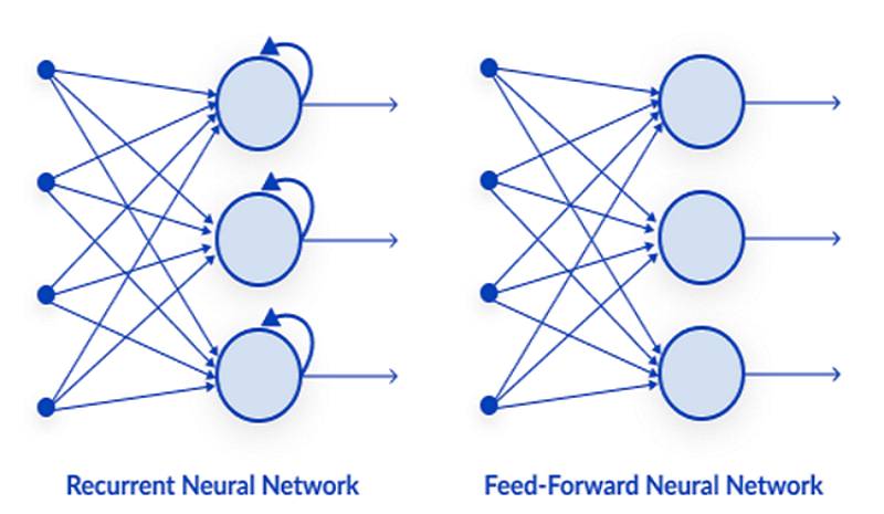
This is one of the simplest types of neural networks. In a feed-forward neural network, the data passes through the different input nodes until it reaches an output node. In contrast to backpropagation, here the data moves in one direction only.
Simply, Backpropagation does the same processes in the neural network as feed-forward where data get passed from the input layer to the output layer except that in back-propagation after the output of the network reaches the output layer it gets to see the real value of a class, and compare it to the value of it has predicted, the model sees how wrong or correct it has made the predictions if it made a wrong prediction it passes the data backward the network and update its parameters so that it predicts corrects the next time. This is a self-taught type of algorithm.
02: Recurrent Neural Network
A recurrent neural network is a type of artificial neural network in which the output of a particular layer is saved and fed back to the input layer. This helps predict the outcome of the layer.
Recurrent neural nets are used to solve problems related to
- Time series data
- Text data
- Audio data
The most common use in text data is recommending the next words for an AI to speak for example: How + are + you +?
03: Convolution Neural Network (CNN)
CNN's are in the rage in the deep learning community. They prevail in image and video processing projects.
For example, image detection and classification AI are composed of convolution neural networks.
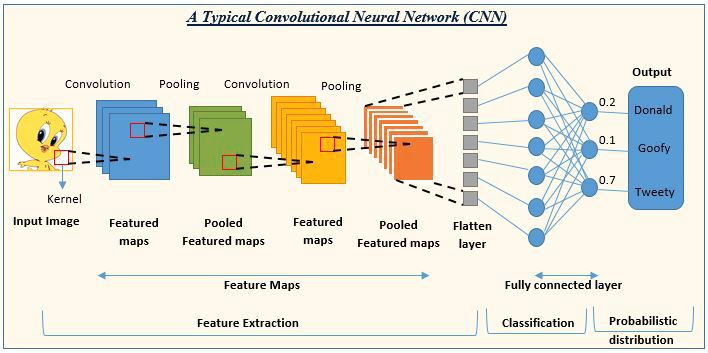
Image source: analyticsvidhya.com
Now that we have seen the types of neural networks, let's shift the focus to this article's main topic Feed Forward Neural Networks.
Feed Forward Neural Networks
Unlike other more complex types of neural networks, there is no backpropagation, meaning data flows in one direction only in this type of neural network. A feed-forward neural net may have a single hidden layer or, several hidden layers.
Let's see what makes this network tick
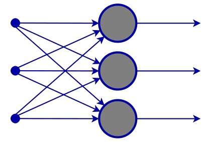
Input Layer
From the images of a neural network, it appears that there is an input layer but deep inside, an input layer is just a presentation. No calculations are performed in the input layer.
Hidden Layer
The hidden layer is where the majority of the work in the network gets done.
To clarify things let's dissect the second hidden layer Node.
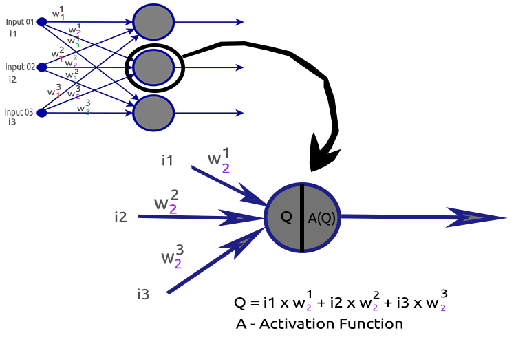
Processes involved:
- Finding the dot product of the inputs and their respective weights
- Adding the dot product obtained to the bias
- The result of the second procedure gets passed to the activation function
What is Bias?
Bias allows you to shift the linear regression up and down to fit the prediction line with the data better. This is the same as the Intercept in a linear regression line.
You will understand this parameter well under the section MLP with a single node in a hidden layer is a linear Regression model.
The importance of bias is well explained in this Stack.
What are the Weights?
Weights reflect how important input is they are the coefficients of the equation which you are trying to resolve. Negative weights reduce the value of the output and vice versa. When a neural network is trained on a training dataset it is initialized with a set of weights. These weights are then optimized during the training period and the optimum value of weights is produced.
What is an Activation Function?
An activation function is nothing but a mathematical function that takes an input and produces an output.
Kinds of Activation Functions
There are many activation functions with their variants but here are the most commonly used ones:
- Relu
- Sigmoid
- TanH
- Softmax
Knowing which activation function to use and where is very important, I can't tell you how many times I have seen articles online suggesting to use an Activation function in a place where it was irrelevant. Let's see this in detail.
01: RELU
RELU stands for Rectified Linear Activation Function.
This is the most used activation function in neural nets. It is the simplest of all, easy to code, and easy to interpret the output, that's why it is so popular. This function will output the input directly if the input is a positive number; otherwise, it outputs zero.
Here is the logic
if x < 0 : return 0
else return x
This function better be used in solving regression problems
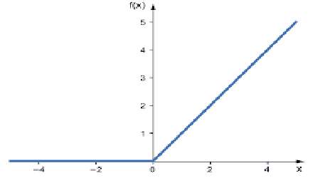
Its output ranges from zero to positive Infinity.
Its MQL5 code is:
double CNeuralNets::Relu(double z)
 {
   if (z < 0) return(0);
   else return(z);
 }
RELU solves the vanishing gradient problem that the sigmoid and TanH suffer (we'll see what this is all about in the article on backpropagation).
02: Sigmoid
Sounds familiar right? Remember from logistic regression.
Its formula is as given below.
![]()
This function is better to be used in classification problems, especially, in classifying one class or two classes only.
Its output ranges from zero to one(Probability terms).
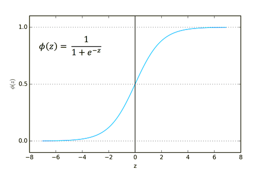
For instance, your network has two nodes in the output. The first node is for a cat and, the other one is for a dog. You might choose the output if the output of the first node is greater than 0.5 to indicate it is a cat and the same but opposite for a dog.
Its MQL5 code is:
double CNeuralNets::Sigmoid(double z)
 {
   return(1.0/(1.0+MathPow(e,-z)));
 }
03: TanH
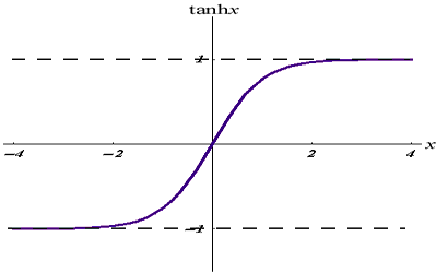
The Hyperbolic Tangent Function.
It's given by the formula:
Its graph looks like the below:
This activation function is similar to the sigmoid but better.
Its output ranges from -1 to 1.
This Function better be used in multiclass classification neural nets
Its MQL5 code is given below:
double CNeuralNets::tanh(double z)
 {
   return((MathPow(e,z) - MathPow(e,-z))/(MathPow(e,z) + MathPow(e,-z)));
 }
04: SoftMax
Someone once asked, why there is no graph for the SoftMax function. Unlike other activation functions, the SoftMax is not used in the hidden layers but in the output layer only and should be used only when you want to convert the output of a multiclass neural network into probability terms.
The SoftMax predicts multinomial probability distribution.

For example, the outputs of a regression neural net are [1,3,2] if we apply the SoftMax function to this output the output now becomes [0.09003, 0.665240, 0.244728].
The output of this function ranges from 0 to 1.
Its MQL5 code will be:
void CNeuralNets::SoftMax(double &Nodes[])
 {
   double TempArr[];
   ArrayCopy(TempArr,Nodes);  ArrayFree(Nodes);

   double proba = 0, sum=0;

   for (int j=0; j<ArraySize(TempArr); j++)    sum += MathPow(e,TempArr[j]);

    for (int i=0; i<ArraySize(TempArr); i++)
      {
         proba = MathPow(e,TempArr[i])/sum;
         Nodes[i] = proba;
     }

    ArrayFree(TempArr);
 }
Now that we understand what a single Neuron of a hidden layer is made up of let's code for it.
void CNeuralNets::Neuron(int HLnodes,
                        double bias,
                        double &Weights[],
                        double &Inputs[],
                        double &Outputs[]
                       )
 {
   ArrayResize(Outputs,HLnodes);

   for (int i=0, w=0; i<HLnodes; i++)
    {
      double dot_prod = 0;
      for(int j=0; j<ArraySize(Inputs); j++, w++)
        {
            if (m_debug) printf("i %d  w %d = input %.2f x weight %.2f",i,w,Inputs[j],Weights[w]);
            dot_prod += Inputs[j]*Weights[w];
        }

      Outputs[i] = ActivationFx(dot_prod+bias);
    }
 }
Inside the ActivationFx(), we have a choice for which activation function was chosen when calling the NeuralNets constructor.
double CNeuralNets::ActivationFx(double Q)
 {
   switch(A_fx)
     {
      case  SIGMOID:
        return(Sigmoid(Q));
        break;
      case TANH:
         return(tanh(Q));
         break;
      case RELU:
         return(Relu(Q));
         break;
      default:
         Print("Unknown Activation Function");
        break;
     }
   return(0);
 }
Further explanations on the code:
The function Neuron() is not just a single node inside the hidden layer but all the operations of a hidden layer are performed inside that one function. The nodes in all hidden layers will have the same size as the input node all the way to the final output node I chose this structure because I'm about to do some classification using this neural network on a random generated dataset.
The below function FeedForwardMLP() is a NxN structure meaning that if you have 3 input nodes and you chose to have 3 hidden layers you will have 3 hidden nodes on each hidden layers see the image.
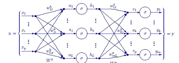
Here is the FeedForwardMLP() Function:
void   CNeuralNets::FeedForwardMLP(int HiddenLayers,
           double &MLPInputs[],
           double &MLPWeights[],
           double &bias[],
           double &MLPOutput[])
 {

    double L_weights[], L_inputs[], L_Out[];

    ArrayCopy(L_inputs,MLPInputs);

    int HLnodes = ArraySize(MLPInputs);
    int no_weights = HLnodes*ArraySize(L_inputs);
    int weight_start = 0;

    for (int i=0; i<HiddenLayers; i++)
      {

        if (m_debug) printf("<< Hidden Layer %d >>",i+1);
        ArrayCopy(L_weights,MLPWeights,0,weight_start,no_weights);

        Neuron(HLnodes,bias[i],L_weights,L_inputs,L_Out);

        ArrayCopy(L_inputs,L_Out);
        ArrayFree(L_Out);

        ArrayFree(L_weights);

        weight_start += no_weights;
      }

    if (use_softmax)  SoftMax(L_inputs);
    ArrayCopy(MLPOutput,L_inputs);
    if (m_debug)
      {
       Print("\nFinal MLP output(s)");
       ArrayPrint(MLPOutput,5);
      }
 }
The operations for finding the dot product in a neural network could be handled by matrix operations but for the sake of keeping things clear and easy for everyone to understand in this first article, I chose the loop method we will use matrix multiplication next time around.
Now that you have seen the architecture I just chose by default for the sake of building the library. This now raises a question about neural networks architecture(s).
If you go to google and search the images of a neural network, you will be bombarded by thousands if not, ten thousand images with different neural nets structures like these for example:

A million-dollar question is, what is the best neural network architecture?
"No one is so wrong as the man who knows all the answers" --Thomas Merton.
Let's break the thing down to understand what's necessary and what's not.
The Input layerThe number of inputs comprising this layer should be equal to the number of features (columns in the dataset).
The Output layer
Determining the size (the number of neurons) is determined by the classes in your dataset for a classification neural network, for a regression type of problem the number of neurons is determined by the chosen model configuration. One output layer for a regressor is often more than enough.
Hidden Layers
If your problem isn't complex enough one or two hidden layers are more than enough, as the matter of fact two hidden layers are sufficient for the large majority of the problems. But, how many nodes do you need in each hidden layer? I'm not sure about this but I think it depends on the performance, this is for you as a developer to explore and try different nodes to see what works best for a particular sort of problem, also before you start playing with this you should acknowledge other types of neural networks we discussed earlier.
There is a great topic on stats.stackexchange.com about this subject linked here.
I think having the same number of nodes as the input layer for all the hidden layers is ideal for a feed-forward neural net, that is the configuration I go with most of the times.
MLP with a single Node and single hidden layer is a Linear model.
If you pay attention to the operations done inside a single node of a hidden layer of a neural network you will notice this:
Q = wi * Ii + b
meanwhile, the linear regression equation is;
Y = mi * xi + c
Notice any similarity? They are the same thing theoretically, this operation is the linear regressor this brings us back to the importance of the bias of a hidden layer. The bias is a constant for the linear model with the role of adding the flexibility of our model to fit the given dataset, without it all models will pass between the x and y axis at zero(0).
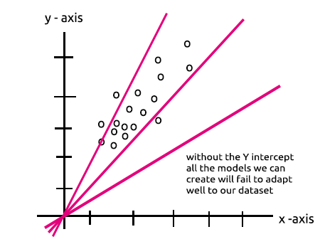
When training the neural network the weights and the biases will be updated. The parameters that produce the less errors for our model will be kept and remembered in the testing dataset.
Now let me build a MLP for two class classification to make points clear. Before that let me generate a random dataset with labelled samples that we are going to see through our neural network. The below function makes random dataset, second sample being multiplied by 5 the first one being multiplied by 2 just to get data on different scales.
void MakeBlobs(int size=10)
 {
     ArrayResize(data_blobs,size);
     for (int i=0; i<size; i++)
       {
         data_blobs[i].sample_1 = (i+1)*(2);

         data_blobs[i].sample_2 = (i+1)*(5);

         data_blobs[i].class_ = (int)round(nn.MathRandom(0,1));
       }
 }
When I print the dataset here is the output:
QK      0       18:27:57.298    TestScript (EURUSD,M1)  CNeural Nets Initialized activation = SIGMOID UseSoftMax = No
IR      0       18:27:57.298    TestScript (EURUSD,M1)      [sample_1] [sample_2] [class_]
LH      0       18:27:57.298    TestScript (EURUSD,M1)  [0]     2.0000     5.0000        0
GG      0       18:27:57.298    TestScript (EURUSD,M1)  [1]     4.0000    10.0000        0
NL      0       18:27:57.298    TestScript (EURUSD,M1)  [2]     6.0000    15.0000        1
HJ      0       18:27:57.298    TestScript (EURUSD,M1)  [3]     8.0000    20.0000        0
HQ      0       18:27:57.298    TestScript (EURUSD,M1)  [4]    10.0000    25.0000        1
OH      0       18:27:57.298    TestScript (EURUSD,M1)  [5]    12.0000    30.0000        1
JF      0       18:27:57.298    TestScript (EURUSD,M1)  [6]    14.0000    35.0000        0
DL      0       18:27:57.298    TestScript (EURUSD,M1)  [7]    16.0000    40.0000        1
QK      0       18:27:57.298    TestScript (EURUSD,M1)  [8]    18.0000    45.0000        0
QQ      0       18:27:57.298    TestScript (EURUSD,M1)  [9]    20.0000    50.0000        0
The next part is to generate random weight values and the bias,
     generate_weights(weights,ArraySize(Inputs));
     generate_bias(biases);
Here is the output:
RG      0       18:27:57.298    TestScript (EURUSD,M1)  weights
QS      0       18:27:57.298    TestScript (EURUSD,M1)   0.7084 -0.3984  0.6182  0.6655 -0.3276  0.8846  0.5137  0.9371
NL      0       18:27:57.298    TestScript (EURUSD,M1)  biases
DD      0       18:27:57.298    TestScript (EURUSD,M1)  -0.5902  0.7384
Now let's see the whole operations in the main Function of our script:
#include "NeuralNets.mqh";
CNeuralNets *nn;

input int batch_size =10;
input int hidden_layers =2;

data data_blobs[];
//+------------------------------------------------------------------+
//| Script program start function                                    |
//+------------------------------------------------------------------+
void OnStart()
  {
//---
     nn = new CNeuralNets(SIGMOID);

     MakeBlobs(batch_size);

     ArrayPrint(data_blobs);

     double Inputs[],OutPuts[];

     ArrayResize(Inputs,2);     ArrayResize(OutPuts,2);

     double weights[], biases[];
     generate_weights(weights,ArraySize(Inputs));
     generate_bias(biases);

     Print("weights"); ArrayPrint(weights);
     Print("biases"); ArrayPrint(biases);

     for (int i=0; i<batch_size; i++)
       {
         Print("Dataset Iteration ",i);
         Inputs[0] = data_blobs[i].sample_1; Inputs[1]= data_blobs[i].sample_2;
         nn.FeedForwardMLP(hidden_layers,Inputs,weights,biases,OutPuts);
       }

     delete(nn);
  }
Things to notice:
- The number of bias is the same as the number of hidden layers.
- Total number of weights = number of inputs squared multiplied to the number of hidden layers. This has been made possible by the fact that our network has the same number of nodes as the input layer/ previous layer of the network (all layers have same number of nodes from the input to the output).
- The same principle will be followed, let's say if you have 3 inputs nodes, all hidden layers will have 3 nodes, except for the last layer where we are about to see how to deal with it.
Looking at the random generated dataset you will notice two input features/ columns in the dataset and I have chosen to have 2 hidden layers, here is the brief overview in our logs of how our model will perform the calculations(prevent these logs by setting debug mode to false in the code).
NL      0       18:27:57.298    TestScript (EURUSD,M1)  Dataset Iteration 0
EJ      0       18:27:57.298    TestScript (EURUSD,M1)  << Hidden Layer 1 >>
GO      0       18:27:57.298    TestScript (EURUSD,M1)
NS      0       18:27:57.298    TestScript (EURUSD,M1)   HLNode 1
EI      0       18:27:57.298    TestScript (EURUSD,M1)  i 0  w 0 = input 2.00000 x weight 0.70837
FQ      0       18:27:57.298    TestScript (EURUSD,M1)  i 0  w 1 = input 5.00000 x weight -0.39838
QP      0       18:27:57.298    TestScript (EURUSD,M1)  dot_Product -0.57513 + bias -0.590 = -1.16534
RH      0       18:27:57.298    TestScript (EURUSD,M1)  Activation function Output =0.23770
CQ      0       18:27:57.298    TestScript (EURUSD,M1)
OE      0       18:27:57.298    TestScript (EURUSD,M1)   HLNode 2
CO      0       18:27:57.298    TestScript (EURUSD,M1)  i 1  w 2 = input 2.00000 x weight 0.61823
FI      0       18:27:57.298    TestScript (EURUSD,M1)  i 1  w 3 = input 5.00000 x weight 0.66553
PN      0       18:27:57.298    TestScript (EURUSD,M1)  dot_Product 4.56409 + bias -0.590 = 3.97388
GM      0       18:27:57.298    TestScript (EURUSD,M1)  Activation function Output =0.98155
DI      0       18:27:57.298    TestScript (EURUSD,M1)  << Hidden Layer 2 >>
GL      0       18:27:57.298    TestScript (EURUSD,M1)
NF      0       18:27:57.298    TestScript (EURUSD,M1)   HLNode 1
FH      0       18:27:57.298    TestScript (EURUSD,M1)  i 0  w 0 = input 0.23770 x weight -0.32764
ID      0       18:27:57.298    TestScript (EURUSD,M1)  i 0  w 1 = input 0.98155 x weight 0.88464
QO      0       18:27:57.298    TestScript (EURUSD,M1)  dot_Product 0.79044 + bias 0.738 = 1.52884
RK      0       18:27:57.298    TestScript (EURUSD,M1)  Activation function Output =0.82184
QG      0       18:27:57.298    TestScript (EURUSD,M1)
IH      0       18:27:57.298    TestScript (EURUSD,M1)   HLNode 2
DQ      0       18:27:57.298    TestScript (EURUSD,M1)  i 1  w 2 = input 0.23770 x weight 0.51367
CJ      0       18:27:57.298    TestScript (EURUSD,M1)  i 1  w 3 = input 0.98155 x weight 0.93713
QJ      0       18:27:57.298    TestScript (EURUSD,M1)  dot_Product 1.04194 + bias 0.738 = 1.78034
JP      0       18:27:57.298    TestScript (EURUSD,M1)  Activation function Output =0.85574
EI      0       18:27:57.298    TestScript (EURUSD,M1)
GS      0       18:27:57.298    TestScript (EURUSD,M1)  Final MLP output(s)
OF      0       18:27:57.298    TestScript (EURUSD,M1)  0.82184 0.85574
CN      0       18:27:57.298    TestScript (EURUSD,M1)  Dataset Iteration 1
KH      0       18:27:57.298    TestScript (EURUSD,M1)  << Hidden Layer 1 >>
EM      0       18:27:57.298    TestScript (EURUSD,M1)
DQ      0       18:27:57.298    TestScript (EURUSD,M1)   HLNode 1
QH      0       18:27:57.298    TestScript (EURUSD,M1)  i 0  w 0 = input 4.00000 x weight 0.70837
PD      0       18:27:57.298    TestScript (EURUSD,M1)  i 0  w 1 = input 10.00000 x weight -0.39838
HR      0       18:27:57.298    TestScript (EURUSD,M1)  dot_Product -1.15027 + bias -0.590 = -1.74048
DJ      0       18:27:57.298    TestScript (EURUSD,M1)  Activation function Output =0.14925
OP      0       18:27:57.298    TestScript (EURUSD,M1)
CK      0       18:27:57.298    TestScript (EURUSD,M1)   HLNode 2
MN      0       18:27:57.298    TestScript (EURUSD,M1)  i 1  w 2 = input 4.00000 x weight 0.61823
NH      0       18:27:57.298    TestScript (EURUSD,M1)  i 1  w 3 = input 10.00000 x weight 0.66553
HI      0       18:27:57.298    TestScript (EURUSD,M1)  dot_Product 9.12817 + bias -0.590 = 8.53796
FO      0       18:27:57.298    TestScript (EURUSD,M1)  Activation function Output =0.99980
RG      0       18:27:57.298    TestScript (EURUSD,M1)  << Hidden Layer 2 >>
IR      0       18:27:57.298    TestScript (EURUSD,M1)
PD      0       18:27:57.298    TestScript (EURUSD,M1)   HLNode 1
RN      0       18:27:57.298    TestScript (EURUSD,M1)  i 0  w 0 = input 0.14925 x weight -0.32764
HF      0       18:27:57.298    TestScript (EURUSD,M1)  i 0  w 1 = input 0.99980 x weight 0.88464
EM      0       18:27:57.298    TestScript (EURUSD,M1)  dot_Product 0.83557 + bias 0.738 = 1.57397
EL      0       18:27:57.298    TestScript (EURUSD,M1)  Activation function Output =0.82835
KE      0       18:27:57.298    TestScript (EURUSD,M1)
GN      0       18:27:57.298    TestScript (EURUSD,M1)   HLNode 2
LS      0       18:27:57.298    TestScript (EURUSD,M1)  i 1  w 2 = input 0.14925 x weight 0.51367
FL      0       18:27:57.298    TestScript (EURUSD,M1)  i 1  w 3 = input 0.99980 x weight 0.93713
KH      0       18:27:57.298    TestScript (EURUSD,M1)  dot_Product 1.01362 + bias 0.738 = 1.75202
IR      0       18:27:57.298    TestScript (EURUSD,M1)  Activation function Output =0.85221
OH      0       18:27:57.298    TestScript (EURUSD,M1)
IM      0       18:27:57.298    TestScript (EURUSD,M1)  Final MLP output(s)
MH      0       18:27:57.298    TestScript (EURUSD,M1)  0.82835 0.85221
Now pay attention to the final MLP output(s) for the all the iterations you will notice a weird behavior that the outputs tend to have neatly the same values. This issue has several causes as discussed in this Stack, one of them being using the wrong activation function in the output layer. This is where the SoftMax activation function comes to the play.
From my understanding the sigmoid function returns probabilities only when there is a single node in the output layer, which it has to classify one class, In this case you would need the output of sigmoid to tell you if something belongs to a certain class or not, but it is another different story in multiclass. If we sum the outputs of our final nodes the value exceeds one(1) most of the times, so now you know they are not probabilities because probability can not exceed the value of 1.
If we apply SoftMax to the last layer the outputs will be.
First Iteration outputs [0.4915 0.5085] , Second Iteration Outputs [0.4940 0.5060]
you can interpret the outputs as [Probability belonging to class 0 Probability belonging to class 1] in this case
Well, at least now we have probabilities that we can rely on to interpret something meaningful from our network.
Final thoughts
We are not through with the feed-forward neural network but at least for now you have an understanding of the theory and most important stuff that will be helpful for you to master neural networks in MQL5. The designed Feedforward neural network is the one for classification purposes so that means the suitable Activation functions are sigmoid and tanh depending on the samples and classes you want to classify in your dataset. We couldn't change the output layer to return whatever we would like to play with it and neither are nodes in the hidden layers, the introduction of matrices will help all this operation to become dynamic so that we can build a very standard neural network for any task, that is a goal of this article series stay tuned for more.
Knowing when to use the neural network is also an important thing because not all the tasks need to be solved by neural nets, if a task can be solved by linear regression, a linear model may outperform the neural network. That is one of the things to keep in mind.
GitHub repo: https://github.com/MegaJoctan/NeuralNetworks-MQL5
Further Reading | Books | References
-
Neural Networks for Pattern Recognition (Advanced Texts in Econometrics)
-
Neural Networks: Tricks of the Trade (Lecture Notes in Computer Science, 7700)
-
Deep Learning (Adaptive Computation and Machine Learning series)
Articles References:
-
Data Science and Machine Learning (Part 01): Linear Regression
-
Data Science and Machine Learning (Part 02): Logistic Regression
-
Data Science and Machine Learning (Part 03): Matrix Regressions
-
Data Science and Machine Learning (Part 06): Gradient Descent
Warning: All rights to these materials are reserved by MetaQuotes Ltd. Copying or reprinting of these materials in whole or in part is prohibited.
This article was written by a user of the site and reflects their personal views. MetaQuotes Ltd is not responsible for the accuracy of the information presented, nor for any consequences resulting from the use of the solutions, strategies or recommendations described.
 Learn how to design a trading system by Bear's Power
 Learn how to design a trading system by Bull's Power
- Free trading apps
- Over 8,000 signals for copying
- Economic news for exploring financial markets
You agree to website policy and terms of use

...
Could you explain it? Or give some examples?
the difference between optimization, on the strategy tester versus optimizing the neural network parameters is the goal, on the strategy tester we tend to focus on the parameters that provide the most profitable outputs or at least the trading results we want, this doesn't necessarily mean that the neural network has a good model that has led to those kind of results
some folks prefer to put the weights and the bias as input parameters of neural net based systems(Feed forward roughly speaking) but I think optimizing using the strategy tester is basically finding the random values of the best results(finding the optimal ones sounds like depending on luck) while if we were to optimize using stochastic gradient descent we are moving towards the model with the least errors in predictions on every step
Thank you for your response.
I got your point.
Why did you start from the first part?
old article:
DATA SCIENCE AND MACHINE LEARNING (PART 01): LINEAR REGRESSION
https://www.mql5.com/en/articles/10459
Why did you start from the first part?
old article:
DATA SCIENCE AND MACHINE LEARNING (PART 01): LINEAR REGRESSION
https://www.mql5.com/en/articles/10459
what do you mean?
Why did you start from the first part?
old article:
DATA SCIENCE AND MACHINE LEARNING (PART 01): LINEAR REGRESSION
https://www.mql5.com/en/articles/10459