
Data Science and ML (Part 46): Stock Markets Forecasting Using N-BEATS in Python

Contents
- What is N-BEATS?
- How does N-BEATS work
- Core goals of the N-BEATS model
- Building the N-BEATS model
- Out-of-sample forecasting using the N-BEATS model
- Multi-series forecasting
- Making Trading Decisions using N-BEATS in MetaTrader 5
- Conclusion
What is N-BEATS?
N-BEATS (Neural Basis Expansion Analysis for Time Series) is a deep learning model specifically designed for time series forecasting. It provides a flexible framework for univariate and multivariate forecasting tasks.
It was introduced by researchers at Element AI (now part of ServiceNow) in 2019, with the paper N-BEATS: Neural basis expansion analysis for interpretable time series forecasting.
Developers at Element AI developed this model to challenge the dominance of classical statistical models like ARIMA and ETS in time series, while compromising the capabilities offered by classical machine learning models.
We all know that time series forecasting is a challenging task, so machine learning experts and users sometimes rely on deep learning models such as RNNs, LSTMs, etc., which are often:
- Overcomplicated for some simple tasks
- Hard to interpret
- They are not consistently outperforming statistical baselines despite their complexity.
Meanwhile, traditional models for time series forecasting, like ARIMA, are often too simple for many tasks.
So, the authors/developers decided to make a deep learning model for time series forecasting that works well, is interpretable, and needs no domain-specific tweaks.

Core Goals of the N-BEATS Model
Developers had clear goals and motivations for creating this machine learning tool; they aimed at addressing limitations in both classical and deep learning-based time series forecasting.
Below is a detailed elaboration of the core goals of N-BEATS:
- Model Simplicity Without Sacrificing Accuracy
Since simpler/linear models for time series forecasting such as ARIMA are unable to capture complex relationships which is better captured by Neural Network based models (deep learning models), developers decided to use simple Neural Network architectures (MLPs) for time series forecasting as they are more interpretable, faster, and easier to debug.
Using deep learning models like (RNNs, LSTMs, or Transformers) introduces a layer of complexity to the system, making the model harder to tune and slow to train. - Interpretability Through Structure
Since MLPs and other Neural Network based models don't provide interpretable results, developers aimed to create a neural-network-based model that can provide human-interpretable forecasts by decomposing the output into trend and seasonal components similar to classical time series models like ETS.
The N-BEATS model allows clear attributions, e.g., "This spike in the data is because of the trend" or "this drop is seasonal", this is achieved via basis expansion layers (like polynomial or Fourier basis). - Competitive Accuracy Without Domain-Specific Tweaks
Another goal that this model aims to accomplish is to design a general-purpose model that works well on a wide range of time series, with minimal manual feature engineering.
This is because models like Prophet require users to specify trend and seasonality patterns.
N-BEATS learns these patterns automatically, directly from the data. - Support Global Modeling Across Many Time Series
Since many models for time series forecasting can forecast a single time series at once (panel data), this model is built to forecast multiple time series.This is very practical because in financial data, we might have more than one feature that we want to forecast. For example, forecasting close prices for NASDAQ and S&P 500 at the same time.
- Fast and Scalable Training
N-BEATS was aimed to make the model fast and easy to parallelize, unlike RNNs or attention-based models. - Strong Baseline Performance
N-BEATS aims to beat state-of-the-art classical methods such as ARIMA and ETS, in a fair, backtested evaluation. - Modular and Extensive Design
Classical models for time series forecasting are static and unmodifiable. N-BEATS comes with an easy-to-modify architecture that allows for the easy addition of custom blocks, such as trend blocks, seasonality blocks, or generic blocks.
Before implementing this model, let's take a brief moment to understand what it's all about.
How does the N-BEATS Model Work (A Brief Mathematical Intuition)
Let us look at the N-BEATS model architecture.
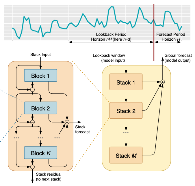
Figure 01
At the top, we have the time series data, which is filtered and processed into several different stacks, from 1 to M stacks.
Each stack is composed of different blocks from 1 to K; from each block, the model produces a forecasted value or a residual, which is then passed to the next stack.
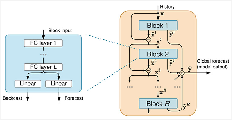
Figure 02
Each block is composed of four fully-connected neural network layers that either produce a backcast or a forecast.
The flow of data into the model
01: In the Stacks
At the very beginning, the model needs to have the lookback period and the forecast period.
The lookback period is how much we look back into the past to predict the future, while the forecast period represents how much we want to predict into the future.
After determining the lookback and forecast period, we start with Stack 01, which takes the lookback period data and begins processing it to make initial predictions. For example, if our lookback period is the past hours' close prices of a certain instrument, Stack 01 uses this data to forecast the next 24 hours.
The obtained initial prediction and its residuals (i.e, actual minus the predicted value) are then passed to the next stack (Stack 02) for further refinement.
This process is repeated for all subsequent stacks until stack M; each stack improving the predictions made by the previous stack.
Finally, the forecasts from all the stacks are combined to produce the global forecast. For example, if Stack 01 predicts a spike, Stack 02 adjusts for trend, and Stack M refines for the long-term patterns. The global forecast integrates all of these insights to give the most accurate prediction possible.
You can think of stacks as different layers of analysis. Stack 01 might focus on capturing short-term patterns, such as hourly fluctuations in the closing prices, while Stack 02 might focus on long-term patterns, such as daily closing prices trends.
Each stack processes the input data to contribute uniquely to the overall forecast.
02: Inside Input Blocks
Starting at Block 01, which takes the stack input, which could be the original lookback data or the residuals from the previous stack, it then uses this input to generate a forecast and a backcast. For example, if the block received the past 24 hours of electricity usage as inputs it produces the forecast for the next 24 hours and the backcast to approximate the input data.
The backcast helps in refining the models' understanding of how the forecast contributes to the overall predictions.
Again, each stack is made up of multiple blocks that work sequentially, so after block one processes the stack input and generates its forecast and backcast, the next one takes in both residuals from the previous block and the original stack input. These two inputs helps the current block make accurate forecasts than the previous one while also considering the original data to enhance the overall accuracy.
This iterative refinement within each block of a stack ensures that the predictions become increasingly accurate through the blocks. After all the blocks within a stack have processed the data, the final residual from the last block (Block K) is passed to the next stack.
03: Dissecting a Block
Within each block the input data is processed through a four layer fully connected stack, this stack transforms the block input extracting features that helps in generating the backcast and the forecast.
The fully conencted layer withing each block is designed to handle data transformations and feature extraction, after the data passes through the fully connected layers it splits into two parts (refer to Figure 02). One part for the backcast and the other for the forecast.
The backcast output aims to approximate the input data, helping to refine the residuals that are passed to the next block, while the forecast output provides predicted values for the forecast period.
Building the N-BEATS model in Python
Start by installing all the modules present in the file requirements.txt found in the attachments table, liked at the end of this article.
pip install -r requirements.txt
Inside test.ipynb, we start by importing all necessary modules.
import MetaTrader5 as mt5
import numpy as np
import matplotlib.pyplot as plt
import pandas as pd
import seaborn as sns
import warnings

sns.set_style("darkgrid")
warnings.filterwarnings("ignore")
Followed by initializing MetaTrader 5.
if not mt5.initialize():
    print("Metratrader5 initialization failed, Error code =", mt5.last_error())
    mt5.shutdown()
We collect 1000 bars from the daily timeframe on the NASDAQ (NAS100) symbol.
rates = mt5.copy_rates_from_pos("NAS100", mt5.TIMEFRAME_D1, 1, 1000)
rates_df = pd.DataFrame(rates)
Despite this model using techniques offered by classical machine learning techniques, which are often multivariate, N-BEATS takes a univariate approach similar to the one deployed in traditional time series models like ARIMA and VAR.
Below is how we construct univariate data.
univariate_df = rates_df[["time", "close"]].copy()
univariate_df["ds"] = pd.to_datetime(univariate_df["time"], unit="s") # convert the time column to datetime
univariate_df["y"] = univariate_df["close"] # closing prices
univariate_df["unique_id"] = "NAS100" # add a unique_id column | very important for univariate models

# Final dataframe
univariate_df = univariate_df[["unique_id", "ds", "y"]].copy()

univariate_df
Outputs.
| unique_id | ds | y | |
|---|---|---|---|
| 0 | NAS100 | 2021-08-30 | 9.655648 |
| 1 | NAS100 | 2021-08-31 | 9.654988 |
| 2 | NAS100 | 2021-09-01 | 9.655763 |
| 3 | NAS100 | 2021-09-02 | 9.654981 |
| 4 | NAS100 | 2021-09-03 | 9.658335 |
| ... | ... | ... | ... |
| 995 | NAS100 | 2025-07-07 | 10.028180 |
| 996 | NAS100 | 2025-07-08 | 10.031142 |
| 997 | NAS100 | 2025-07-09 | 10.037376 |
| 998 | NAS100 | 2025-07-10 | 10.036098 |
| 999 | NAS100 | 2025-07-11 | 10.033283 |
univariate_df["unique_id"] = "NAS100" # add a unique_id column | very important for univariate models
The neuralforecast module, which has the N-BEATS model, is designed to handle both univariate and panel (multi-series) forecasting. The unique_id feature tells the model which time series each row belongs to. This is especially critical when:
- You are forecasting multiple assets or symbols (e.g., AAPL, TSLA, MSFT, EURUSD).
- You want to batch train a single model on many time series.
This variable is mandatory (even for a single series) because of internal grouping and indexing mechanisms.
It takes a few lines of code to train this model.
from neuralforecast import NeuralForecast
from neuralforecast.models import NBEATS # Neural Basis Expansion Analysis for Time Series

# Define model and horizon
horizon = 30  # forecast 30 days into the future

model = NeuralForecast(
    models=[NBEATS(h=horizon, # predictive horizon of the model
                   input_size=90, # considered autorregresive inputs (lags), y=[1,2,3,4] input_size=2 -> lags=[1,2].
                   max_steps=100, # maximum number of training steps (epochs)
                   scaler_type='robust', # scaler type for the time series data
                   )],
    freq='D' # frequency of the time series data
)

# Fit the model
model.fit(df=univariate_df)
Outputs.
Seed set to 1
GPU available: False, used: False
TPU available: False, using: 0 TPU cores
HPU available: False, using: 0 HPUs

  | Name         | Type          | Params | Mode
-------------------------------------------------------
0 | loss         | MAE           | 0      | train
1 | padder_train | ConstantPad1d | 0      | train
2 | scaler       | TemporalNorm  | 0      | train
3 | blocks       | ModuleList    | 2.6 M  | train
-------------------------------------------------------
2.6 M     Trainable params
7.3 K     Non-trainable params
2.6 M     Total params
10.541    Total estimated model params size (MB)
31        Modules in train mode
0         Modules in eval mode

Epoch 99: 100%
 1/1 [00:01<00:00,  0.88it/s, v_num=32, train_loss_step=0.259, train_loss_epoch=0.259]
`Trainer.fit` stopped: `max_steps=100` reached.
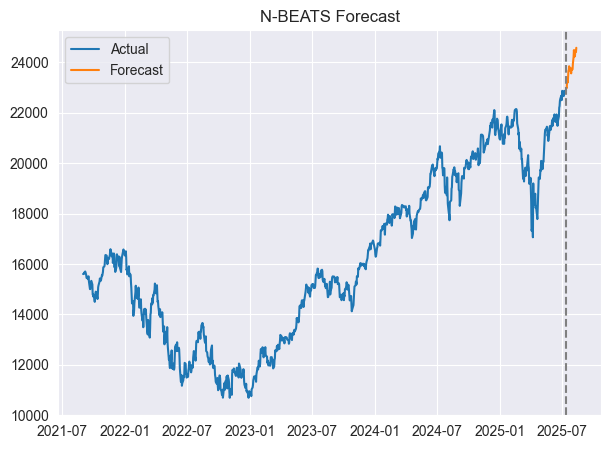
We can visualize the predictions and actual values on the same axis.
forecast = model.predict() # predict future values based on the fitted model

# Merge forecast with original data
plot_df = pd.merge(univariate_df, forecast, on='ds', how='outer')

plt.figure(figsize=(7,5))
plt.plot(plot_df['ds'], plot_df['y'], label='Actual')
plt.plot(plot_df['ds'], plot_df['NBEATS'], label='Forecast')
plt.axvline(plot_df['ds'].max() - pd.Timedelta(days=horizon), color='gray', linestyle='--')
plt.legend()
plt.title('N-BEATS Forecast')
plt.show()
Outputs.
Below is an appearance of the merged dataframe.
| unique_id_x | ds | y | unique_id_y | NBEATS | |
|---|---|---|---|---|---|
| 0 | NAS100 | 2021-08-31 | 15599.4 | NaN | NaN |
| 1 | NAS100 | 2021-09-01 | 15611.5 | NaN | NaN |
| 2 | NAS100 | 2021-09-02 | 15599.3 | NaN | NaN |
| 3 | NAS100 | 2021-09-03 | 15651.7 | NaN | NaN |
| 4 | NAS100 | 2021-09-06 | 15700.4 | NaN | NaN |
| ... | ... | ... | ... | ... | ... |
| 1025 | NaN | 2025-08-09 | NaN | NAS100 | 24235.187500 |
| 1026 | NaN | 2025-08-10 | NaN | NAS100 | 24466.316406 |
| 1027 | NaN | 2025-08-11 | NaN | NAS100 | 24454.646484 |
| 1028 | NaN | 2025-08-12 | NaN | NAS100 | 24405.820312 |
| 1029 | NaN | 2025-08-13 | NaN | NAS100 | 24571.919922 |
Great, the model has predicted 30 days into the future.
For evaluation purposes, let's train this model on one dataset and test it on the other, as we always evaluate any typical machine learning model.
Out-of-sample Forecasting Using the N-BEATS Model
We start by splitting the data into training and testing dataframes.
split_date = '2024-01-01'  # the split date for training and testing

train_df = univariate_df[univariate_df['ds'] < split_date]
test_df = univariate_df[univariate_df['ds'] >= split_date]
We train the model on the training dataset.
model = NeuralForecast(
    models=[NBEATS(h=horizon, # predictive horizon of the model
                   input_size=90, # considered autorregresive inputs (lags), y=[1,2,3,4] input_size=2 -> lags=[1,2].
                   max_steps=100, # maximum number of training steps (epochs)
                   scaler_type='robust', # scaler type for the time series data
                   )],
    freq='D' # frequency of the time series data
)

# Fit the model
model.fit(df=train_df)
Since the predict function predicts the next "N" number of days forward according to the predictive horizon, to evaluate this model on out-of-sample forecasts, we have to merge the predicted outcome dataframe alongside the actual dataframe.
test_forecast = model.predict() # predict future 30 days based on the training data

df_test = pd.merge(test_df, test_forecast, on=['ds', 'unique_id'], how='outer') # merge the test data with the forecast
df_test.dropna(inplace=True) # drop rows with NaN values

df_test
Outputs.
| unique_id | ds | y | NBEATS | |
|---|---|---|---|---|
| 3 | NAS100 | 2024-01-02 | 16554.3 | 16569.835938 |
| 4 | NAS100 | 2024-01-03 | 16368.1 | 16596.839844 |
| 5 | NAS100 | 2024-01-04 | 16287.2 | 16603.513672 |
| 6 | NAS100 | 2024-01-05 | 16307.1 | 16729.607422 |
| 9 | NAS100 | 2024-01-08 | 16631.0 | 16854.746094 |
| 10 | NAS100 | 2024-01-09 | 16672.4 | 16918.466797 |
| 11 | NAS100 | 2024-01-10 | 16804.7 | 16958.833984 |
| 12 | NAS100 | 2024-01-11 | 16814.3 | 17130.972656 |
| 13 | NAS100 | 2024-01-12 | 16808.8 | 17055.396484 |
| 16 | NAS100 | 2024-01-15 | 16828.7 | 17272.376953 |
| 17 | NAS100 | 2024-01-16 | 16841.9 | 17227.498047 |
| 18 | NAS100 | 2024-01-17 | 16727.7 | 17408.158203 |
| 19 | NAS100 | 2024-01-18 | 16987.0 | 17499.619141 |
| 20 | NAS100 | 2024-01-19 | 17336.7 | 17318.767578 |
| 23 | NAS100 | 2024-01-22 | 17329.3 | 17399.562500 |
| 24 | NAS100 | 2024-01-23 | 17426.1 | 17289.140625 |
| 25 | NAS100 | 2024-01-24 | 17503.1 | 17236.478516 |
| 26 | NAS100 | 2024-01-25 | 17469.4 | 17188.691406 |
| 27 | NAS100 | 2024-01-26 | 17390.1 | 17315.134766 |
We proceed to evaluate this outcome.
from sklearn.metrics import mean_absolute_percentage_error, r2_score

mape = mean_absolute_percentage_error(df_test['y'], df_test['NBEATS'])
r2_score_ = r2_score(df_test['y'], df_test['NBEATS'])

print(f"mean_absolute_percentage_error (MAPE): {mape} \n R2 Score: {r2_score_}")
Outputs.
mean_absolute_percentage_error (MAPE): 0.015779373328172166
R2 Score: 0.35350182943487285
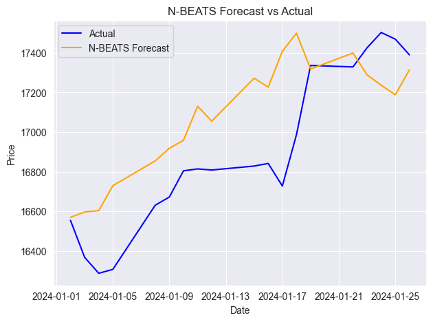
According to the MAPE metric, model predictions are very accurate in percentage terms; meanwhile, the R2 score value of 0.35 means that only 35% of the variation in the target variable is explained.
Below is the plot containing actual and forecasted values on a single axis.
Just like any other time series forecasting model, N-BEATS needs to be updated regularly with new sequential data to remain relevant and accurate. In the previous examples, we have evaluated the model based on the forecasts made 30 days ahead on the daily timeframe data but, this isn't the right way as the model misses a lot of daily information in between.
The right way is be to update the model with new data as soon as new data appears.
The N-BEATS model provides an easy way to update the model with new data without re-training it, which saves a lot of time.
When you run:
NBEATS.predict(df=new_dataframe) The model applies the trained weights on the new data as it runs an inference of the model, which updates the model with new information, making it relevant to the recently received data from a dataframe.
Multi-Series Forecasting
As described earlier, in the core goals of the N-BEATS section. This model is designed to handle multi-series forecasting in the best possible way.
This is an impressive ability of this model because it leverages patterns learned on one series and uses them to improve the overall forecast for both time series.
Below is how you can harness this ability:
We start by collecting data for each symbol from MetaTrader 5.
rates_nq = mt5.copy_rates_from_pos("NAS100", mt5.TIMEFRAME_D1, 1, 1000)
rates_df_nq = pd.DataFrame(rates_nq)

rates_snp = mt5.copy_rates_from_pos("US500", mt5.TIMEFRAME_D1, 1, 1000)
rates_df_snp = pd.DataFrame(rates_snp)
We prepare each separate univariate Dataframe.
# NAS100
rates_df_nq["ds"] = pd.to_datetime(rates_df_nq["time"], unit="s")
rates_df_nq["y"] = rates_df_nq["close"]
rates_df_nq["unique_id"] = "NAS100"
df_nq = rates_df_nq[["unique_id", "ds", "y"]]

# US500
rates_df_snp["ds"] = pd.to_datetime(rates_df_snp["time"], unit="s")
rates_df_snp["y"] = rates_df_snp["close"]
rates_df_snp["unique_id"] = "US500"
df_snp = rates_df_snp[["unique_id", "ds", "y"]]
We combine both dataframes and sort the values according to the data column and their unique_id.
multivariate_df = pd.concat([df_nq, df_snp], ignore_index=True) # combine both dataframes
multivariate_df = multivariate_df.sort_values(['unique_id', 'ds']).reset_index(drop=True) # sort by unique_id and date

multivariate_df
Outputs.
| unique_id | ds | y | |
|---|---|---|---|
| 0 | NAS100 | 2021-08-31 | 15599.4 |
| 1 | NAS100 | 2021-09-01 | 15611.5 |
| 2 | NAS100 | 2021-09-02 | 15599.3 |
| 3 | NAS100 | 2021-09-03 | 15651.7 |
| 4 | NAS100 | 2021-09-06 | 15700.4 |
| ... | ... | ... | ... |
| 1995 | US500 | 2025-07-08 | 6229.9 |
| 1996 | US500 | 2025-07-09 | 6264.9 |
| 1997 | US500 | 2025-07-10 | 6280.3 |
| 1998 | US500 | 2025-07-11 | 6255.8 |
| 1999 | US500 | 2025-07-14 | 6271.9 |
Like we did previously, we split the data into training and testing Dataframes.
split_date = '2024-01-01'  # the split date for training and testing

train_df = multivariate_df[multivariate_df['ds'] < split_date]
test_df = multivariate_df[multivariate_df['ds'] >= split_date]
Then, we train the model in the same way as we did prior.
from neuralforecast import NeuralForecast
from neuralforecast.models import NBEATS # Neural Basis Expansion Analysis for Time Series

# Define model and horizon
horizon = 30  # forecast 30 days into the future

model = NeuralForecast(
    models=[NBEATS(h=horizon, # predictive horizon of the model
                   input_size=90, # considered autorregresive inputs (lags), y=[1,2,3,4] input_size=2 -> lags=[1,2].
                   max_steps=100, # maximum number of training steps (epochs)
                   scaler_type='robust', # scaler type for the time series data
                   )],
    freq='D' # frequency of the time series data
)

# Fit the model
model.fit(df=train_df)
We make forecast on out-of-sample data.
test_forecast = model.predict() # predict future 30 days based on the training data

df_test = pd.merge(test_df, test_forecast, on=['ds', 'unique_id'], how='outer') # merge the test data with the forecast
df_test.dropna(inplace=True) # drop rows with NaN values

df_test
Outputs.
| unique_id | ds | y | NBEATS | |
|---|---|---|---|---|
| 6 | NAS100 | 2024-01-02 | 16554.3 | 16267.765625 |
| 7 | US500 | 2024-01-02 | 4747.4 | 4706.230957 |
| 8 | NAS100 | 2024-01-03 | 16368.1 | 16230.808594 |
| 9 | US500 | 2024-01-03 | 4707.3 | 4706.517090 |
| 10 | NAS100 | 2024-01-04 | 16287.2 | 16136.568359 |
| 11 | US500 | 2024-01-04 | 4690.9 | 4686.380859 |
| 12 | NAS100 | 2024-01-05 | 16307.1 | 16218.930664 |
| 13 | US500 | 2024-01-05 | 4695.8 | 4704.896484 |
Finally, we evaluate the model on both instruments and visualize actual values and the forecasted ones in the same axis.
from sklearn.metrics import mean_absolute_percentage_error, r2_score

unique_ids = df_test['unique_id'].unique()

for unique_id in unique_ids:

    df_unique = df_test[df_test['unique_id'] == unique_id].copy()

    mape = mean_absolute_percentage_error(df_unique['y'], df_unique['NBEATS'])
    r2_score_ = r2_score(df_unique['y'], df_unique['NBEATS'])


    print(f"Unique ID: {unique_id} - MAPE: {mape}, R2 Score: {r2_score_}")


    plt.figure(figsize=(7, 4))
    plt.plot(df_unique['ds'], df_unique['y'], label='Actual', color='blue')
    plt.plot(df_unique['ds'], df_unique['NBEATS'], label='Forecast', color='orange')
    plt.title(f'Actual vs Forecast for {unique_id}')
    plt.xlabel('Date')
    plt.ylabel('Value')
    plt.legend()
    plt.show()
Outputs.
Unique ID: NAS100 - MAPE: 0.0221775184381915, R2 Score: -0.16976266747298419

Unique ID: US500 - MAPE: 0.007412931117247571, R2 Score: 0.3782229067061038

Making Trading Decisions using N-BEATS in MetaTrader 5
Now that we are capable of getting predictions from this model, we can integrate it into a Python-based trading robot.
Inside the file NBEATS-tradingbot.py, we start by implementing the function for training the entire model initially:
def train_nbeats_model(forecast_horizon: int=30,
                       start_bar: int=1,
                       number_of_bars: int=1000,
                       input_size: int=90,
                       max_steps: int=100,
                       mt5_timeframe: int=mt5.TIMEFRAME_D1,
                       symbol_01: str="NAS100",
                       symbol_02: str="US500",
                       test_size_percentage: float=0.2,
                       scaler_type: str='robust'):

    """
        Train NBEATS model on NAS100 and US500 data from MetaTrader 5.

        Args:
            start_bar: starting bar to be used to in CopyRates from MT5
            number_of_bars: The number of bars to extract from MT5 for training the model
            forecast_horizon: the number of days to predict in the future
            input_size: number of previous days to consider for prediction
            max_steps: maximum number of training steps (epochs)
            mt5_timeframe: timeframe to be used for the data extraction from MT5
            symbol_01: unique identifier for the first symbol (default is NAS100)
            symbol_02: unique identifier for the second symbol (default is US500)
            test_size_percentage: percentage of the data to be used for testing (default is 0.2)
            scaler_type: type of scaler to be used for the time series data (default is 'robust')

        Returns:
            NBEATS: the n-beats model object
    """

    # Getting data from MetaTrader 5

    rates_nq = mt5.copy_rates_from_pos(symbol_01, mt5_timeframe, start_bar, number_of_bars)
    rates_df_nq = pd.DataFrame(rates_nq)

    rates_snp = mt5.copy_rates_from_pos(symbol_02, mt5_timeframe, start_bar, number_of_bars)
    rates_df_snp = pd.DataFrame(rates_snp)

    if rates_df_nq.empty or rates_df_snp.empty:
        print(f"Failed to retrieve data for {symbol_01} or {symbol_02}.")
        return None

    # Getting NAS100 data
    rates_df_nq["ds"] = pd.to_datetime(rates_df_nq["time"], unit="s")
    rates_df_nq["y"] = rates_df_nq["close"]
    rates_df_nq["unique_id"] = symbol_01
    df_nq = rates_df_nq[["unique_id", "ds", "y"]]

    # Getting US500 data
    rates_df_snp["ds"] = pd.to_datetime(rates_df_snp["time"], unit="s")
    rates_df_snp["y"] = rates_df_snp["close"]
    rates_df_snp["unique_id"] = symbol_02
    df_snp = rates_df_snp[["unique_id", "ds", "y"]]

    multivariate_df = pd.concat([df_nq, df_snp], ignore_index=True) # combine both dataframes
    multivariate_df = multivariate_df.sort_values(['unique_id', 'ds']).reset_index(drop=True) # sort by unique_id and date

    # Group by unique_id and split per group
    train_df_list = []
    test_df_list = []

    for _, group in multivariate_df.groupby('unique_id'):
        group = group.sort_values('ds')
        split_idx = int(len(group) * (1 - test_size_percentage))

        train_df_list.append(group.iloc[:split_idx])
        test_df_list.append(group.iloc[split_idx:])

    # Concatenate all series
    train_df = pd.concat(train_df_list).reset_index(drop=True)
    test_df = pd.concat(test_df_list).reset_index(drop=True)

    # Define model and horizon

    model = NeuralForecast(
        models=[NBEATS(h=forecast_horizon, # predictive horizon of the model
                    input_size=input_size, # considered autorregresive inputs (lags), y=[1,2,3,4] input_size=2 -> lags=[1,2].
                    max_steps=max_steps, # maximum number of training steps (epochs)
                    scaler_type=scaler_type, # scaler type for the time series data
                    )],
        freq='D' # frequency of the time series data
    )

    # fit the model on the training data

    model.fit(df=train_df)

    test_forecast = model.predict() # predict future 30 days based on the training data

    df_test = pd.merge(test_df, test_forecast, on=['ds', 'unique_id'], how='outer') # merge the test data with the forecast
    df_test.dropna(inplace=True) # drop rows with NaN values


    unique_ids = df_test['unique_id'].unique()
    for unique_id in unique_ids:

        df_unique = df_test[df_test['unique_id'] == unique_id].copy()

        mape = mean_absolute_percentage_error(df_unique['y'], df_unique['NBEATS'])
        print(f"Unique ID: {unique_id} - MAPE: {mape:.2f}")

    return model
This function combines all the training procedures discussed previously and returns the N-BEATS model object for direct forecasts.
The function for predicting next values takes a similar approach to the one used in the training function.
def predict_next(model,
                  symbol_unique_id: str,
                  input_size: int=90):

    """
        Predict the next values for a given unique_id using the trained model.

        Args:
            model (NBEATS): the trained NBEATS model
            symbol_unique_id (str): unique identifier for the symbol to predict
            input_size (int): number of previous days to consider for prediction

        Returns:
            DataFrame: containing the predicted values for the next days
    """

    # Getting data from MetaTrader 5

    rates = mt5.copy_rates_from_pos(symbol_unique_id, mt5.TIMEFRAME_D1, 1, input_size * 2)  # Get enough data for prediction
    if rates is None or len(rates) == 0:
        print(f"Failed to retrieve data for {symbol_unique_id}.")
        return pd.DataFrame()

    rates_df = pd.DataFrame(rates)

    rates_df["ds"] = pd.to_datetime(rates_df["time"], unit="s")
    rates_df = rates_df[["ds", "close"]].rename(columns={"close": "y"})
    rates_df["unique_id"] = symbol_unique_id
    rates_df = rates_df.sort_values(by="ds").reset_index(drop=True)

    # Prepare the dataframe for reference & prediction
    univariate_df = rates_df[["unique_id", "ds", "y"]]
    forecast = model.predict(df=univariate_df)

    return forecast
We give the model data size twice to the input_size used during training — Just to give it enough data.
Let's call the predict function twice for every separate symbol and observe the resulting dataframes.
trained_model = train_nbeats_model(max_steps=10)

print(predict_next(trained_model, "NAS100").head())
print(predict_next(trained_model, "US500").head())
Outputs.
Predicting DataLoader 0: 100%|████████████████████████████████████████████████████████████████████████████████████████████████| 1/1 [00:00<00:00, 45.64it/s]
  unique_id         ds        NBEATS
0    NAS100 2025-07-16  22836.160156
1    NAS100 2025-07-17  22931.242188
2    NAS100 2025-07-18  22984.792969
3    NAS100 2025-07-19  23037.224609
4    NAS100 2025-07-20  23119.804688
GPU available: False, used: False
TPU available: False, using: 0 TPU cores
HPU available: False, using: 0 HPUs
Predicting DataLoader 0: 100%|████████████████████████████████████████████████████████████████████████████████████████████████| 1/1 [00:00<00:00, 71.43it/s]
  unique_id         ds       NBEATS
0     US500 2025-07-16  6234.584961
1     US500 2025-07-17  6254.846680
2     US500 2025-07-18  6261.153320
3     US500 2025-07-19  6282.960449
4     US500 2025-07-20  6307.293945
GPU available: False, used: False
TPU available: False, using: 0 TPU cores
HPU available: False, using: 0 HPUs
Since the resulting dataframes for both symbols contain multiple daily closing price predictions for 30 days ahead (Today's date is 16.07.2025), we have to select a value predicted for the current day (Today's date).
today = dt.datetime.now().date() # today's date

forecast_df = predict_next(trained_model, "NAS100") # Get the predicted values for NAS100, 30 days into the future
today_pred_close_nq = forecast_df[forecast_df['ds'].dt.date == today]['NBEATS'].values # extract today's predicted close value for NAS100

forecast_df = predict_next(trained_model, "US500") # Get the predicted values for US500, 30 days into the future
today_pred_close_snp = forecast_df[forecast_df['ds'].dt.date == today]['NBEATS'].values # extract today's predicted close value for US500

print(f"Today's predicted NAS100 values:", today_pred_close_nq)
print(f"Today's predicted US500 values:", today_pred_close_snp)
Outputs.
Today's predicted NAS100 values: [22836.16]
Today's predicted US500 values: [6234.585]
Finally, we can use these predicted values in a simple trading strategy.
# Trading modules

from Trade.Trade import CTrade
from Trade.PositionInfo import CPositionInfo
from Trade.SymbolInfo import CSymbolInfo

SLIPPAGE = 100 # points
MAGIC_NUMBER = 15072025 # unique identifier for the trades
TIMEFRAME = mt5.TIMEFRAME_D1 # timeframe for the trades

# Create trade objects for NAS100 and US500
m_trade_nq = CTrade(magic_number=MAGIC_NUMBER,
                 filling_type_symbol = "NAS100",
                 deviation_points=SLIPPAGE)

m_trade_snp = CTrade(magic_number=MAGIC_NUMBER,
                 filling_type_symbol = "US500",
                 deviation_points=SLIPPAGE)

# Training the NBEATS model INITIALLY
trained_model = train_nbeats_model(max_steps=10,
                                    input_size=90,
                                    forecast_horizon=30,
                                    start_bar=1,
                                    number_of_bars=1000,
                                    mt5_timeframe=TIMEFRAME,
                                    symbol_01="NAS100",
                                    symbol_02="US500"
                                   )

m_symbol_nq = CSymbolInfo("NAS100") # Create symbol info object for NAS100
m_symbol_snp = CSymbolInfo("US500") # Create symbol info object for US500

m_position = CPositionInfo() # Create position info object


def pos_exists(pos_type: int, magic: int, symbol: str) -> bool:

    """ Checks whether a position exists given a magic number, symbol, and the position type

    Returns:
        bool: True if a position is found otherwise False
    """

    if mt5.positions_total() < 1: # no positions whatsoever
        return False

    positions = mt5.positions_get()

    for position in positions:
        if m_position.select_position(position):
            if m_position.magic() == magic and m_position.symbol() == symbol and m_position.position_type()==pos_type:
                return True

    return False


def RunStrategyandML(trained_model: NBEATS):

    today = dt.datetime.now().date() # today's date

    forecast_df = predict_next(trained_model, "NAS100") # Get the predicted values for NAS100, 30 days into the future
    today_pred_close_nq = forecast_df[forecast_df['ds'].dt.date == today]['NBEATS'].values # extract today's predicted close value for NAS100

    forecast_df = predict_next(trained_model, "US500") # Get the predicted values for US500, 30 days into the future
    today_pred_close_snp = forecast_df[forecast_df['ds'].dt.date == today]['NBEATS'].values # extract today's predicted close value for US500

    # convert numpy arrays to float values

    today_pred_close_nq = float(today_pred_close_nq[0]) if len(today_pred_close_nq) > 0 else None
    today_pred_close_snp = float(today_pred_close_snp[0]) if len(today_pred_close_snp) > 0 else None

    print(f"Today's predicted NAS100 values:", today_pred_close_nq)
    print(f"Today's predicted US500 values:", today_pred_close_snp)

    # Refreshing the rates for NAS100 and US500 symbols

    m_symbol_nq.refresh_rates()
    m_symbol_snp.refresh_rates()

    ask_price_nq = m_symbol_nq.ask() # get today's close price for NAS100
    ask_price_snp = m_symbol_snp.ask() # get today's close price for US500

    # Trading operations for the NAS100 symol

    if not pos_exists(pos_type=mt5.ORDER_TYPE_BUY, magic=MAGIC_NUMBER, symbol="NAS100"):
        if today_pred_close_nq > ask_price_nq: # if predicted close price for NAS100 is greater than the current ask price
            # Open a buy trade
            m_trade_nq.buy(volume=m_symbol_nq.lots_min(),
                            symbol="NAS100",
                            price=m_symbol_nq.ask(),
                            sl=0.0,
                            tp=today_pred_close_nq) # set take profit to the predicted close price

    print("ask: ", m_symbol_nq.ask(), "bid: ", m_symbol_nq.bid(), "last: ", ask_price_nq)
    print("tp: ", today_pred_close_nq, "lots: ", m_symbol_nq.lots_min())
    print("istp within range: ", (m_symbol_nq.ask() - today_pred_close_nq) > m_symbol_nq.stops_level())

    if not pos_exists(pos_type=mt5.ORDER_TYPE_SELL, magic=MAGIC_NUMBER, symbol="NAS100"):
        if today_pred_close_nq < ask_price_nq: # if predicted close price for NAS100 is less than the current bid price
            m_trade_nq.sell(volume=m_symbol_nq.lots_min(),
                             symbol="NAS100",
                             price=m_symbol_nq.bid(),
                             sl=0.0,
                             tp=today_pred_close_nq) # set take profit to the predicted close price


    # Buy and sell operations for the US500 symbol


    if not pos_exists(pos_type=mt5.ORDER_TYPE_BUY, magic=MAGIC_NUMBER, symbol="US500"):
        if today_pred_close_snp > ask_price_snp: # if the predicted price for US500 is greater than the current ask price
            m_trade_snp.buy(volume=m_symbol_snp.lots_min(),
                            symbol="US500",
                            price=m_symbol_snp.ask(),
                            sl=0.0,
                            tp=today_pred_close_snp)

    if not pos_exists(pos_type=mt5.ORDER_TYPE_SELL, magic=MAGIC_NUMBER, symbol="US500"):
        if today_pred_close_snp < ask_price_snp: # if the predicted price for US500 is less than the current bid price
            m_trade_snp.sell(volume=m_symbol_snp.lots_min(),
                             symbol="US500",
                             price=m_symbol_snp.bid(),
                             sl=0.0,
                             tp=today_pred_close_snp)


RunStrategyandML(trained_model=trained_model) # Run the strategy and ML model once to initialize
Outputs.
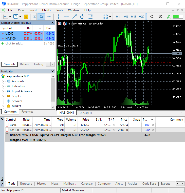
Two new trades were opened.
Finally, we can schedule the training progress and automate the model to make predictions and open trades at the beginning of every day.
# Schedule the strategy to run every day at 00:00
schedule.every().day.at("00:00").do(RunStrategyandML, trained_model=trained_model)

while True:

    schedule.run_pending()
    time.sleep(10)
Conclusion
N-BEATS is a powerful model for time series analysis and forecasting. It surpasses classical models such as ARIMA, VAR, PROPHET, etc, for the same task, since it leverages neural networks at their core which excel in capturing complex patterns.
N-BEATS is a perfect alternative for those wanting to perform time series forecasting using non-traditional models for time series forecasting.
I love that it comes with normalization techniques and evaluation tools in its toolbox, making this model convenient to use.
While it is a decent model, just like any machine learning model in the world, it has some drawbacks which should be acknowledged, including:
- They are designed primarily for univariate forecasting
As seen previously, they primarily require two features only in the training dataframe ds (datestamp) and the target variable marked as y. Similar to the PROPHET model discussed previously.
In financial data these two features aren't enough to capture the market dynamics. - They can overfit on noisy data
Like other deep networks, N-BEATS can overfit in noisy data. - It's interpretability is limited
While N-BEATS includes a basis function decomposition for interpretability, it is still a deep neural network; it is less interpretable than other models for time series forecasting like ARIMA and PROPHET. - It is less widely adopted in the Industry
You've probably never heard of this model before.
Although it's strong in academic benchmarks, this model hasn't been widely adopted in the machine learning community compared to other models like ARIMA, XGBoost, LSTM's etc. You won't find many posts online describing this model.
Best regards.
Attachments Table
| Filename | Description & Usage |
|---|---|
| Trade\PositionInfo.py | Contains the CPositionInfo class similarly to the one available in MQL5; the class provides information about all opened positions in MetaTrader 5. |
| Trade\SymbolInfo.py | Contains the CSymbolInfo class similarly to the one available in MQL5; the class provides all information about the selected symbol from MetaTrader 5. |
| Trade\Trade.py | Contains the CTrade class similarly to the one available in MQL5; the class provides functions for opening and closing trades in MetaTrader 5. |
| error_description.py | Has the functions for converting MetaTrader 5 error codes into Human-readable information. |
| NBEATS-Tradingbot.py | A Python script that uses the N-BEATS model to make trading decisions. |
| test.ipynb | A Jupyter Notebook for experimenting with the N-BEATS model. |
| requirements.txt | Contains all the Python dependencies used in this project. |
Sources & References
Warning: All rights to these materials are reserved by MetaQuotes Ltd. Copying or reprinting of these materials in whole or in part is prohibited.
This article was written by a user of the site and reflects their personal views. MetaQuotes Ltd is not responsible for the accuracy of the information presented, nor for any consequences resulting from the use of the solutions, strategies or recommendations described.

- Free trading apps
- Over 8,000 signals for copying
- Economic news for exploring financial markets
You agree to website policy and terms of use
Check out the new article: Data Science and ML (Part 46): Stock Markets Forecasting Using N-BEATS in Python.
Author: Omega J Msigwa