
数据科学与机器学习(第43篇):使用潜在高斯混合模型(LGMM)识别指标数据中的隐藏模式

内容
- 引言
- 什么是潜在高斯混合模型
- LGMM 背后的数学原理
- 用指标数据训练 LGMM
- 基于 LGMM 的 MQL5 指标
- 为 LGMM 寻找最优分量数量
- 潜在高斯混合模型与分类器模型结合使用
- 基于 LGMM 的交易机器人
- 结论
引言
作为交易者,我们使用的几乎所有交易策略,都基于某种模式识别和检测。我们研究指标以寻找模式和确认信号,有时甚至会绘制对象和线条,比如支撑线和阻力线,来判断市场状态。
虽然人类易于在金融市场中识别模式,但由于市场的本质(充满噪声和混沌),要将这一过程编程并自动化却极具挑战性。
一些交易者已经开始采用人工智能(AI)和机器学习来完成这项特定任务,他们使用各种基于计算机视觉的技术,像人类一样处理图像数据,正如前文所述。
在本文中,我们将探讨一种名为潜在高斯混合模型(LGMM)的概率模型,它具备检测模式的能力。我们将研究该模型在给定指标数据的情况下,在金融市场中检测隐藏模式和做出准确预测的有效性。

什么是潜在高斯混合模型(LGMM)?
潜在高斯混合模型是一种概率模型,它假设数据是由多个高斯分布混合生成的,每个分布都与一个潜在(隐藏)变量相关联。
它是高斯混合模型(GMM)的扩展,纳入了用于解释每个观测值聚类归属的潜在变量。
潜在高斯模型用于分析这样一类数据:生成数据的底层过程无法直接观测,且假设其服从高斯(正态)分布。
"潜在" 部分指的是这些未被观测到的变量,就像电路中看不见的电信号 —— 它们影响着系统的行为,却无法被直接测量。
在金融市场中,这些潜在变量可以代表数据中底层的交易模式,而我们常常误读或错过这些模式。
简而言之,LGMM 的核心要素包括:
- 潜在变量
这些是假设服从高斯分布的未观测变量,代表影响观测数据的底层因素。 - 观测值
即实际观测到的数据。它通常不服从高斯分布,而是通过某个已知函数与潜在变量建立联系,并可呈现为任意分布。 - 参数
这些参数支配着潜在变量与观测值之间的关系,包括分布的均值和方差。
LGMM 背后的数学原理
LGMM 是一种概率生成模型,其核心是聚类技术。它包含:
潜在变量
- 这些变量无法被直接观测
- 它们代表数据点所属的分量(聚类)
- 它们通常被建模为类别(离散)分布,例如:

混合模型
数据的概率分布是多个高斯分布的加权和。

其中:
-
 πₖ 表示第 k 个分量的混合系数(先验概率),且所有 πₖ 之和为 1
 ,
, 
-
 𝒩(μₖ, Σₖ) = 均值为 μₖ、
 协方差
协方差 为 Σₖ的高斯分布
潜在变量表示
我们不直接对 p (x) 建模,而是考虑:
![]()
其中:
该模型的目标是估计潜在变量和参数 θ![]() 。
。
确定这些变量最常用的方法是期望最大化(EM)算法。
LGMM 的期望最大化(EM)算法
这包括两个步骤:期望步和最大化步。
步骤 01:期望。
这一步涉及估计每个数据点属于每个高斯分布的后验概率。

步骤 02:最大化
这一步涉及使用 γ(zₙₖ) 来更新参数![]() 。
。


在训练过程中,步骤 01 和步骤 02 会重复执行,直到模型收敛。
LGMM 已在现实世界中应用于多个领域,例如带不确定性的数据聚类(软聚类)、异常检测、密度估计以及语音识别相关任务。
用指标数据训练 LGMM
我们知道,在指标数据中存在着各种模式,作为交易者,我们利用这些模式来做出明智的交易决策。我们的目标是首先使用 LGMM 来检测这些模式。
我们首先使用 MQL5 语言从 MetaTrader 5 收集指标数据。
- 交易品种:XAUUSD(黄金兑美元)
- 时间周期:日线(DAILY)
文件名:Get XAUUSD Data.mq5
#include <Arrays\ArrayString.mqh>
#include <Arrays\ArrayObj.mqh>
#include <pandas.mqh> //https://www.mql5.com/en/articles/17030

input datetime start_date = D'2005.01.01';
input datetime end_date = D'2023.01.01';

input string symbol = "XAUUSD";
input ENUM_TIMEFRAMES timeframe = PERIOD_D1;

struct indicator_struct
 {
   long handle;
   CArrayString buffer_names; //buffer_names array
 };

indicator_struct indicators[15]; //Structure for keeping indicator handle alongside its buffer names
//+------------------------------------------------------------------+
//| Script program start function                                    |
//+------------------------------------------------------------------+
void OnStart()
  {
//---

   vector time, open, high, low, close;
   if (!SymbolSelect(symbol, true))
      {
         printf("%s failed to select symbol %s, Error = %d",__FUNCTION__,symbol,GetLastError());
         return;
      }

 //---

   time.CopyRates(symbol, timeframe, COPY_RATES_TIME, start_date, end_date);
   open.CopyRates(symbol, timeframe, COPY_RATES_OPEN, start_date, end_date);
   high.CopyRates(symbol, timeframe, COPY_RATES_HIGH, start_date, end_date);
   low.CopyRates(symbol, timeframe, COPY_RATES_LOW, start_date, end_date);
   close.CopyRates(symbol, timeframe, COPY_RATES_CLOSE, start_date, end_date);

   CDataFrame df;

   df.insert("Time", time);
   df.insert("Open", open);
   df.insert("High", high);
   df.insert("Low", low);
   df.insert("Close", close);

//--- Oscillators

   indicators[0].handle = iATR(symbol, timeframe, 14);
   indicators[0].buffer_names.Add("ATR");

   indicators[1].handle = iBearsPower(symbol, timeframe, 13);
   indicators[1].buffer_names.Add("BearsPower");

   indicators[2].handle = iBullsPower(symbol, timeframe, 13);
   indicators[2].buffer_names.Add("BullsPower");

   indicators[3].handle = iChaikin(symbol, timeframe, 3, 10, MODE_EMA, VOLUME_TICK);
   indicators[3].buffer_names.Add("Chainkin");

   indicators[4].handle = iCCI(symbol, timeframe, 14, PRICE_OPEN);
   indicators[4].buffer_names.Add("CCI");

   indicators[5].handle = iDeMarker(symbol, timeframe, 14);
   indicators[5].buffer_names.Add("Demarker");

   indicators[6].handle = iForce(symbol, timeframe, 13, MODE_SMA, VOLUME_TICK);
   indicators[6].buffer_names.Add("Force");

   indicators[7].handle = iMACD(symbol, timeframe, 12, 26, 9, PRICE_OPEN);
   indicators[7].buffer_names.Add("MACD MAIN_LINE");
   indicators[7].buffer_names.Add("MACD SIGNAL_LINE");

   indicators[8].handle = iMomentum(symbol, timeframe, 14, PRICE_OPEN);
   indicators[8].buffer_names.Add("Momentum");

   indicators[9].handle = iOsMA(symbol, timeframe, 12, 26, 9, PRICE_OPEN);
   indicators[9].buffer_names.Add("OsMA");

   indicators[10].handle = iRSI(symbol, timeframe, 14, PRICE_OPEN);
   indicators[10].buffer_names.Add("RSI");

   indicators[11].handle = iRVI(symbol, timeframe, 10);
   indicators[11].buffer_names.Add("RVI MAIN_LINE");
   indicators[11].buffer_names.Add("RVI SIGNAL_LINE");

   indicators[12].handle = iStochastic(symbol, timeframe, 5, 3,3,MODE_SMA,STO_LOWHIGH);
   indicators[12].buffer_names.Add("StochasticOscillator MAIN_LINE");
   indicators[12].buffer_names.Add("StochasticOscillator SIGNAL_LINE");

   indicators[13].handle = iTriX(symbol, timeframe, 14, PRICE_OPEN);
   indicators[13].buffer_names.Add("TEMA");

   indicators[14].handle = iWPR(symbol, timeframe, 14);
   indicators[14].buffer_names.Add("WPR");

//--- Get buffers

   for (uint ind=0; ind<indicators.Size(); ind++) //Loop through all the indicators
      {
         for (uint buffer_no=0; buffer_no<(uint)indicators[ind].buffer_names.Total(); buffer_no++) //Their buffer names resemble their buffer numbers
            {
               string name = indicators[ind].buffer_names.At(buffer_no); //Get the name of the buffer, it is helpful for the DataFrame and CSV file

               vector buffer = {};
               if (!buffer.CopyIndicatorBuffer(indicators[ind].handle, buffer_no, start_date, end_date)) //Copy indicator buffer
                  {
                     printf("func=%s line=%d | Failed to copy %s indicator buffer, Error = %d",__FUNCTION__,__LINE__,name,GetLastError());
                     continue;
                  }

               df.insert(name, buffer); //Insert a buffer vector and its name to a dataframe object
            }
      }

   df.to_csv(StringFormat("Oscillators.%s.%s.csv",symbol,EnumToString(timeframe)), true); //Save all the data to a CSV file
  }
输出。
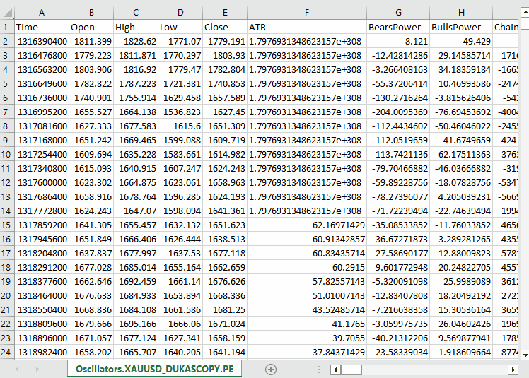
请注意,我们收集了 MQL5 中几乎所有内置的震荡指标,其中大多数恰好会产生较平稳的序列,因为它们通常有最小值和最大值。例如:RSI 指标产生的值在 0 到 100 之间。
尽管 LGMM 能够处理具有不同统计特性的数据,例如非平稳数据。但平稳数据使 LGMM 更容易找到有意义的结构和模式,因为平稳数据的统计特性随时间保持不变。
您可以自由选择任意偏好的数据类型。
我们收集了开盘价、最高价、最低价、收盘价和时间(OHLCT)变量以及指标数据,用于机器学习。这些信息除了用于 LGMM 外,还可用于可视化以及为预测性机器学习模型构建目标变量。
在 Python 脚本(Jupyter Notebook)中,我们做的第一件事就是在导入依赖项并初始化 MetaTrader 5 桌面应用程序后,立即加载这些数据。
Filename: main.ipynb
import pandas as pd
import numpy as np
import MetaTrader5 as mt5
import os
from Trade.TerminalInfo import CTerminalInfo
import matplotlib.pyplot as plt
import seaborn
import warnings

warnings.filterwarnings("ignore")
seaborn.set_style("darkgrid")

if not mt5.initialize():
    print("Failed to Initialize MetaTrade5, Error = ",mt5.last_error())
    mt5.shutdown()


terminal = CTerminalInfo() # similarly to CTerminalInfo from MQL5. 用于获取 MetaTrader 5 应用程序的信息
我们从公共路径(文件夹)中导入数据,也就是我们使用 MQL5 保存数据的位置。
common_path = os.path.join(terminal.common_data_path(), "Files")
symbol = "XAUUSD"
timeframe = "PERIOD_D1"

df = pd.read_csv(os.path.join(common_path, f"Oscillators.{symbol}.{timeframe}.csv")) # the same naming pattern as the one used in the MQL5 script

# Identify max float value
max_float = np.finfo(float).max

# Replace all max float (double) values with NaN produced by preliminary indicator calculations
df = df.replace(max_float, np.nan)
df.dropna(inplace=True)
df["Time"] = pd.to_datetime(df["Time"], unit="s")

df.head()
输出。
        Time    Open    High    Low     Close   ATR     BearsPower      BullsPower      Chainkin        CCI     ...     MACD SIGNAL_LINE        Momentum        OsMA    RSI     RVI MAIN_LINE   RVI SIGNAL_LINE StochasticOscillator MAIN_LINE  StochasticOscillator SIGNAL_LINE        TEMA    WPR
0       2005-01-03      438.45  438.71  426.72  429.55  5.481429        -12.314215      -0.324215       -1079.046551    -51.013015      ...     0.175727        99.870165       -0.582169       46.666555       -0.082596       0.018515        26.976532       32.920132       -0.000089       -85.144357
1       2005-01-04      429.52  430.18  423.71  427.51  5.450000        -13.677899      -7.207899       -1129.324384    -235.622347     ...     -0.000779       98.615544       -1.252741       37.393138       -0.158362       -0.048541       22.158658       27.150101       -0.000190       -82.774252
2       2005-01-05      427.50  428.77  425.10  426.58  5.162143        -10.743913      -7.073913       -1496.644248    -196.837418     ...     -0.247283       97.044402       -1.816758       35.666584       -0.227422       -0.119850       17.070979       22.068723       -0.000325       -86.990027
3       2005-01-06      426.31  427.85  420.17  421.37  5.234286        -13.606211      -5.926211       -3349.884147    -164.038728     ...     -0.576309       97.480164       -2.194161       34.651526       -0.269634       -0.187300       14.096364       17.775334       -0.000482       -95.312500
4       2005-01-07      421.39  425.48  416.57  419.02  5.605000        -15.098181      -6.188181       -4970.426959    -168.301515     ...     -1.015433       95.440750       -2.669414       30.754440       -0.305796       -0.243045       11.442611       14.203318       -0.000670       -91.609589
让我们为分类问题准备目标变量,以便后续在分类器机器学习模型中使用。在此过程中,我们剔除了非指标特征。
lookahead = 1

df["future_close"] = df["Close"].shift(-lookahead)
new_df = df.dropna()

new_df["Direction"] = np.where(new_df["future_close"]>new_df["Close"], 1, -1) # if a the close value in the next bar(s)=lookahead is above the current close price, thats a long signal otherwise that's a short signal
from sklearn.model_selection import train_test_split

X = new_df.drop(columns=[
    "Time",
    "Open",
    "High",
    "Low",
    "Close",
    "future_close",
    "Direction"
])

y = new_df["Direction"]

X_train, X_test, y_train, y_test = train_test_split(X, y, test_size=0.2, shuffle=True, random_state=42)
我们必须检查以确保拥有所需的 "指标数据"。
X_train.head()
输出。
        ATR     BearsPower      BullsPower      Chainkin        CCI     Demarker        MACD MAIN_LINE  MACD SIGNAL_LINE        Momentum        OsMA    RSI     RVI MAIN_LINE   RVI SIGNAL_LINE StochasticOscillator MAIN_LINE  StochasticOscillator SIGNAL_LINE        TEMA    WPR
1057    30.139286       34.958195       62.858195       16280.794393    268.371098      251356.076923   -1.759289       -15.645899      107.768519      13.886610       62.077386       0.229591        0.108028        92.301971       83.886543       -0.002663       -8.048595
3806    3.096429        0.724299        3.314299        -1279.189840    69.806094       696.923077      -0.121217       -0.952863       100.299538      0.831645        52.157089       0.096237        0.080054        67.031250       71.466497       -0.000077       -21.325052
38884   5.927143        -8.488258       -3.858258       -2005.866698    -213.672289     -3333.080000    -0.049837       0.496440        99.774916       -0.546277       39.550361       -0.022395       0.035070        28.046540       49.606252       0.000012        -73.130342
10351   2.060714        -0.491108       1.158892        723.246254      40.384615       2508.735385     1.293179        0.953618        100.533084      0.339561        58.791715       0.217352        0.294053        57.239819       69.770534       0.000123        -19.070322
38170   5.632143        -5.682364       -3.262364       -1321.008995    -109.039933     -1673.607692    -0.609996       0.785433        99.712893       -1.395429       41.917705       -0.062258       -0.053202       13.322009       9.490964        0.000035        -77.826942
最后训练LGMM。
from sklearn.mixture import GaussianMixture
from skl2onnx import convert_sklearn
from skl2onnx.common.data_types import FloatTensorType

components = 3

gmm = GaussianMixture(n_components=components, covariance_type="full", random_state=42)
gmm.fit(X_train)

latent_features_train = gmm.predict_proba(X_train)
latent_features_test = gmm.predict_proba(X_test)
我为高斯混合模型使用了 3 个分量,希望它能将指标中观察到的模式划分成 3 个聚类。按理说,一个分量对应看涨状态,另一个对应看跌状态,第三个对应盘整/震荡状态。重申一下 ,这只是猜测。
与其他无监督机器学习和聚类技术类似,模型产生的分量(结果)很难解释。目前,我们只能假设每个分量对应我刚才描述的三个类别之一。
你可能会好奇,为什么我把这个模型称为潜在高斯混合模型(LGMM),但最终部署的却是来自 Scikit-Learn 的 GaussianMixture 模型?
导入的 GaussianMixture 模型在功能上与本文数学部分描述的 LGMM 是等效的。这两者在理论上是相同的。
让我们打印 latent_features_train 数组。
latent_features_train
输出。
array([[9.48947877e-13, 1.08107288e-62, 1.00000000e+00],
       [9.71935407e-01, 2.80542130e-02, 1.03801388e-05],
       [5.35722226e-03, 9.94642667e-01, 1.10916653e-07],
       ...,
       [7.72441751e-08, 8.80712550e-41, 9.99999923e-01],
       [9.99975623e-01, 1.07924534e-33, 2.43771745e-05],
       [1.91968188e-01, 8.08030586e-01, 1.22621110e-06]], shape=(3760, 3))
LGMM 在每一行预测中生成了一个包含 3 个元素的数组,每一列代表接收到的数据输入属于 3 个聚类之一的概率。所有 3 列的概率之和在每一行都等于 1。
由于目前这样很难解释,让我们将此模型转换为 ONNX 格式,在 MQL5 中可视化聚类,看看能从这个概率模型的输出中得出什么结论。
基于潜在高斯混合模型(LGMM)的 MQL5 指标
我们首先将 LGMM 保存为 ONNX 格式。
# Define input type (shape should match your training data)
initial_type = [("float_input", FloatTensorType([None, X_train.shape[1]]))]

# Convert the pipeline to ONNX format
onnx_model = convert_sklearn(gmm, initial_types=initial_type)

# Save the model to a file
with open(os.path.join(common_path, f"LGMM.{symbol}.{timeframe}.onnx"), "wb") as f:
    f.write(onnx_model.SerializeToString())
以下是在 Netron 中打开时的模型架构图。
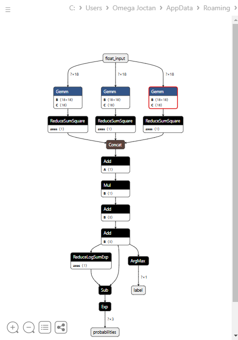
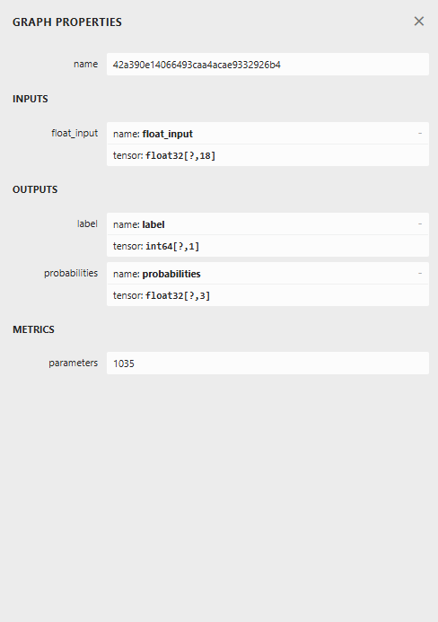
这个模型的架构较为特殊,最终节点有两个输出:一个用于预测标签,另一个用于概率。在 MQL5 中实现加载此模型的代码时,我们需要记住这一点。
在 MQL5 中加载 LGMM
文件名:Gaussian Mixture.mqh
我们需要能够容纳多个数值数组的输出结构,以适配两个输出节点,每个节点都有一个输出数组。
class CGaussianMixture
  {
protected:

   bool initialized;
   long onnx_handle;
   void PrintTypeInfo(const long num,const string layer,const OnnxTypeInfo& type_info);

   ulong inputs[]; //Inputs of a model in dimensions [nxn]
   struct outputs_struct
    {
      ulong outputs[];
    } model_output_structure[];  //Outputs of the model structure array
接着:
bool CGaussianMixture::OnnxLoad(long &handle)
 {
//--- since not all sizes defined in the input tensor we must set them explicitly
//--- first index - batch size, second index - series size, third index - number of series (only Close)

   OnnxTypeInfo type_info; //Getting onnx information for Reference In case you forgot what the loaded ONNX is all about

   long input_count=OnnxGetInputCount(handle);
   if (MQLInfoInteger(MQL_DEBUG))
      Print("model has ",input_count," input(s)");

   for(long i=0; i<input_count; i++)
     {
      string input_name=OnnxGetInputName(handle,i);
      if (MQLInfoInteger(MQL_DEBUG))
         Print(i," input name is ",input_name);

      if(OnnxGetInputTypeInfo(handle,i,type_info))
        {
          if (MQLInfoInteger(MQL_DEBUG))
            PrintTypeInfo(i,"input",type_info);
          ArrayCopy(inputs, type_info.tensor.dimensions);
        }
     }

   long output_count=OnnxGetOutputCount(handle);
   if (MQLInfoInteger(MQL_DEBUG))
      Print("model has ",output_count," output(s)");

   ArrayResize(model_output_structure, (int)output_count);

   for(long i=0; i<output_count; i++)
     {
      string output_name=OnnxGetOutputName(handle,i);
      if (MQLInfoInteger(MQL_DEBUG))
         Print(i," output name is ",output_name);

      if(OnnxGetOutputTypeInfo(handle,i,type_info))
       {
         if (MQLInfoInteger(MQL_DEBUG))
            PrintTypeInfo(i,"output",type_info);

         ArrayCopy(model_output_structure[i].outputs, type_info.tensor.dimensions);
       }

       //--- Set the output shape

         replace(model_output_structure);
         if(!OnnxSetOutputShape(handle, i, model_output_structure[i].outputs))
          {
            if (MQLInfoInteger(MQL_DEBUG))
              {
                printf("Failed to set the Output[%d] shape Err=%d",i,GetLastError());
                DebugBreak();
              }

             return false;
          }
     }

//---

   replace(inputs);

//--- Setting the input size

   for (long i=0; i<input_count; i++)
     if (!OnnxSetInputShape(handle, i, inputs)) //Giving the Onnx handle the input shape
       {
         if (MQLInfoInteger(MQL_DEBUG))
           printf("Failed to set the input shape Err=%d",GetLastError());
         DebugBreak();
         return false;
       }


   initialized = true;
   if (MQLInfoInteger(MQL_DEBUG))
      Print("ONNX model Initialized");

   return true;
 }
//+------------------------------------------------------------------+
//|                                                                  |
//+------------------------------------------------------------------+
bool CGaussianMixture::Init(string onnx_filename, uint flags=ONNX_DEFAULT)
 {
   onnx_handle = OnnxCreate(onnx_filename, flags);

   if (onnx_handle == INVALID_HANDLE)
     return false;

   return OnnxLoad(onnx_handle);
 }
//+------------------------------------------------------------------+
//|                                                                  |
//+------------------------------------------------------------------+
bool CGaussianMixture::Init(const uchar &onnx_buff[], ulong flags=ONNX_DEFAULT)
 {
  onnx_handle = OnnxCreateFromBuffer(onnx_buff, flags); //creating onnx handle buffer

   if (onnx_handle == INVALID_HANDLE)
     return false;

  return OnnxLoad(onnx_handle);
 }
我们将该类的 predict 方法设计为返回两个变量:预测标签和一个包含在结构体中的概率向量。
struct pred_struct
 {
   vector proba;
   long label;
 };
pred_struct CGaussianMixture::predict(const vector &x)
 {
   pred_struct res;

   if (!this.initialized)
    {
      if (MQLInfoInteger(MQL_DEBUG))
         printf("%s The model is not initialized yet to make predictions | call Init function first",__FUNCTION__);

      return res;
    }

//---

   vectorf x_float; //Convert inputs from a vector of double values to those float values
   x_float.Assign(x);

   vector label = vector::Zeros(model_output_structure[0].outputs[1]); //outputs[1] we get the second shape (columns) from an array
   vector proba = vector::Zeros(model_output_structure[1].outputs[1]); //outputs[1] we get the second shape (columns) from an array

   if (!OnnxRun(onnx_handle, ONNX_DATA_TYPE_FLOAT, x_float, label, proba)) //Run the model and get the predicted label and probability
     {
       if (MQLInfoInteger(MQL_DEBUG))
          printf("Failed to get predictions from Onnx err %d",GetLastError());

       DebugBreak();
       return res;
     }

//---

   res.label = (long)label[label.Size()-1]; //Get the last item available at the label's array
   res.proba = proba;

   return res;
 }
让我们在指标的主函数中调用 predict 函数,以获取潜在特征。
文件名:LGMM Indicator.mq5
int OnCalculate(const int32_t rates_total,
                const int32_t prev_calculated,
                const datetime &time[],
                const double &open[],
                const double &high[],
                const double &low[],
                const double &close[],
                const long &tick_volume[],
                const long &volume[],
                const int32_t &spread[])
  {
//--- Main calculation loop

   int lookback = 20;

   for (int i = prev_calculated; i < rates_total && !IsStopped(); i++)
   {
      if (i+1<lookback) //prevent data not found errors during copy buffer
         continue;

      int reverse_index = rates_total - 1 - i;

      //--- Get the indicators data

      vector x = getX(reverse_index, lookback);

      if (x.Size()==0)
         continue;

      pred_struct res = lgmm.predict(x);

      vector proba = res.proba;
      long label = res.label;

      ProbabilityBuffer[i] = proba.Max();

      // Determine color based on histogram value

      if (label == 0)
         ColorBuffer[i] = 0;
      else if (label == 1)
         ColorBuffer[i] = 1;
      else
         ColorBuffer[i] = 2;

      Comment("bars [",i+1,"/",rates_total,"]"," Proba: ",proba," label: ",label);
   }

//---
   return(rates_total);
  }
在 getX () 函数内部,我们必须以与训练数据收集脚本中相同的方式收集所有指标缓冲区。
vector getX(uint start=0, uint count=10)
 {
//--- Get buffers

   CDataFrame df;
   for (uint ind=0; ind<indicators.Size(); ind++) //Loop through all the indicators
      {
        uint buffers_total = indicators[ind].buffer_names.Total();

         for (uint buffer_no=0; buffer_no<buffers_total; buffer_no++) //Their buffer names resemble their buffer numbers
            {
               string name = indicators[ind].buffer_names.At(buffer_no); //Get the name of the buffer, it is helpful for the DataFrame and CSV file

               vector buffer = {};
               if (!buffer.CopyIndicatorBuffer(indicators[ind].handle, buffer_no, start, count)) //Copy indicator buffer
                  {
                     printf("func=%s line=%d | Failed to copy %s indicator buffer, Error = %d",__FUNCTION__,__LINE__,name,GetLastError());
                     continue;
                  }

               df.insert(name, buffer); //Insert a buffer vector and its name to a dataframe object
            }
      }

   return df.iloc(-1); //Return the latest information from the dataframe which is the most recent buffer
 }
注:所有指标都是在 Init 函数中、模型从公共文件夹加载完成后立即初始化的 —— 公共文件夹就是我们用 Python 保存模型的位置。
#include <Gaussian Mixture.mqh>
#include <Arrays\ArrayString.mqh>
#include <MALE5\Pandas\pandas.mqh>

CGaussianMixture lgmm;

input string symbol = "XAUUSD";
input ENUM_TIMEFRAMES timeframe = PERIOD_D1;

struct indicator_struct
 {
   long handle;
   CArrayString buffer_names;
 };

indicator_struct indicators[15];

//--- Indicator buffers

double ProbabilityBuffer[];
double ColorBuffer[];
double MaBuffer[];
//+------------------------------------------------------------------+
//| Custom indicator initialization function                         |
//+------------------------------------------------------------------+
int OnInit()
  {
//--- indicator buffers mapping

   Comment("");

   // Setting indicator properties
   SetIndexBuffer(0, ProbabilityBuffer, INDICATOR_DATA);
   SetIndexBuffer(1, ColorBuffer, INDICATOR_COLOR_INDEX);

   // Setting histogram drawing style
   PlotIndexSetInteger(0, PLOT_DRAW_TYPE, DRAW_COLOR_HISTOGRAM);

   // Set indicator labels
   IndicatorSetString(INDICATOR_SHORTNAME, "3-Color Histogram");
   IndicatorSetInteger(INDICATOR_DIGITS, _Digits);

//---

   string filename = StringFormat("LGMM.%s.%s.onnx",symbol, EnumToString(timeframe));
   if (!lgmm.Init(filename, ONNX_COMMON_FOLDER))
      {
         printf("%s Failed to initialize the GaussianMixture model (LGMM) in ONNX format file={%s}, Error = %d",__FUNCTION__,filename,GetLastError());
      }

//--- Oscillators

   indicators[0].handle = iATR(symbol, timeframe, 14);
   indicators[0].buffer_names.Add("ATR");

   //...
   //...
   //...

   indicators[14].handle = iWPR(symbol, timeframe, 14);
   indicators[14].buffer_names.Add("WPR");

   for (uint i=0; i<indicators.Size(); i++)
     if (indicators[i].handle==INVALID_HANDLE)
        {
          printf("%s Invalid %s handle, Error = %d",__FUNCTION__,indicators[i].buffer_names[0],GetLastError());
          return INIT_FAILED;
        }

//---
   return(INIT_SUCCEEDED);
  }
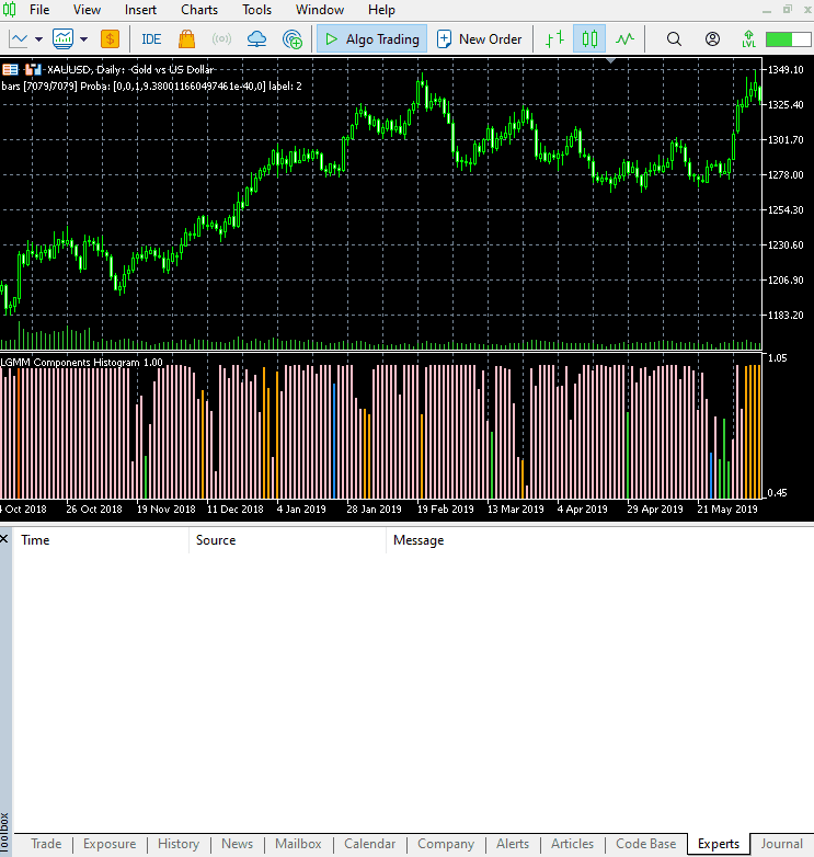
最后,我们在 XAUUSD 图表上运行这个指标,使用的时间周期与模型训练时相同。
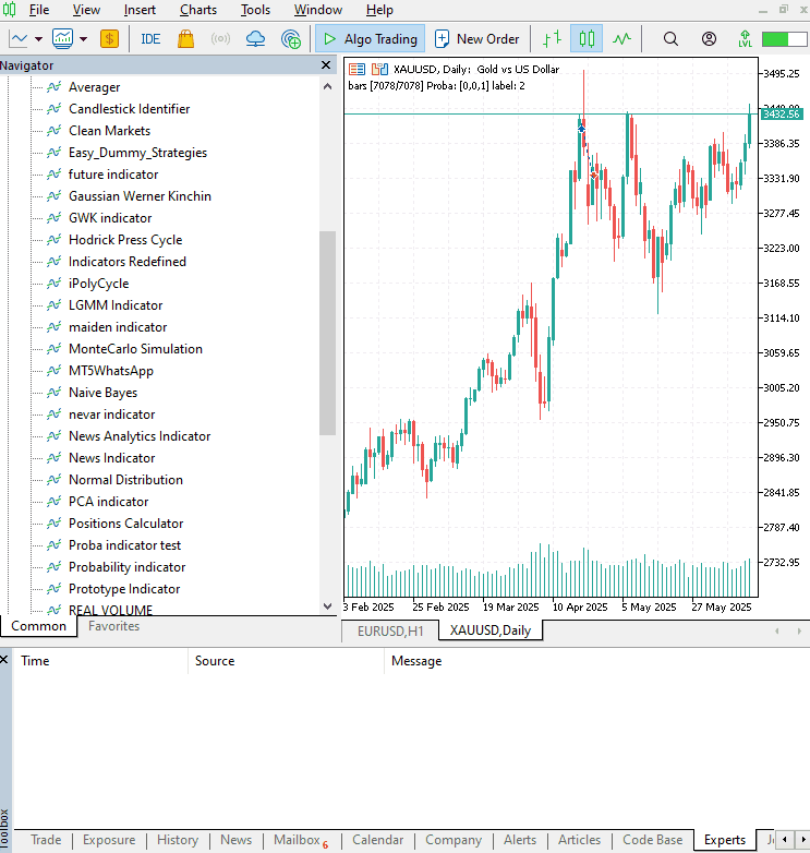
这个指标仍然很难解释,但有一种模式似乎占主导地位,那就是红色呈现的分量。这种模式似乎出现在市场波动剧烈(波动率高)的时候,无论是上升趋势还是下降趋势。其余分量目前还不明确,这可能是因为我们不确定该模型使用的分量数量是否合适。因此,让我们为这个模型寻找最佳的分量数量。
为 LGMM 寻找最佳分量数量
由于 Scikit-Learn 提供的混合模型会输出信息准则值 —— 赤池信息准则(AIC)和贝叶斯信息准则(BIC)。让我们将这些值与其对应的分量数量范围绘制在同一张图上,找出肘部点。
图中的肘部点是指:向模型添加更多分量只会带来性能边际改善的那个点,也就是说,曲线趋于平缓。
文件名:main.ipynb
lowest_bic = np.inf
bic = []
aic = []
n_components_range = range(1, 10)

for n_components in n_components_range:
    gmm = GaussianMixture(n_components=n_components, random_state=42)
    gmm.fit(X)
    bic.append(gmm.bic(X_train))
    aic.append(gmm.aic(X_train))
    if bic[-1] < lowest_bic:
        best_gmm = gmm
        lowest_bic = bic[-1]

# Plot the BIC and AIC scores
plt.figure(figsize=(8, 5))
plt.plot(n_components_range, bic, label='BIC', marker='o')
plt.plot(n_components_range, aic, label='AIC', marker='o')
plt.xlabel('Number of components')
plt.ylabel('Score')
plt.title('LGMM selection: AIC vs BIC')
plt.legend()
plt.grid(True)
plt.show()
输出。

AIC 和 BIC 曲线在分量数从 1 增加到 2 时都急剧下降,随后继续下降,但两者在 5 个分量之后的改善速率都明显放缓。这意味着我们应该为该模型使用的最佳分量数量是 5。
让我们回去重新训练模型,并更新指标。
文件名:main.ipynb
components = 5 # according to the elbow point

gmm = GaussianMixture(n_components=components, covariance_type="full", random_state=42)
gmm.fit(X_train)

latent_features_train = gmm.predict_proba(X_train)
latent_features_test = gmm.predict_proba(X_test)
现在我们有 5 个分量而不是 3 个,也就是说模型会生成 5 个可以绘制的概率值,因此我们需要将指标中彩色直方图的颜色数量增加到 5 种,并为预测标签处理 5 种不同的情况。
文件名:LGMM Indicator.mq5
#property indicator_color1 clrDodgerBlue, clrLimeGreen, clrCrimson, clrOrange, clrYellow
在 OnCalculate 函数内部。
int OnCalculate(const int32_t rates_total,
                const int32_t prev_calculated,
                const datetime &time[],
                const double &open[],
                const double &high[],
                const double &low[],
                const double &close[],
                const long &tick_volume[],
                const long &volume[],
                const int32_t &spread[])
  {
//--- Main calculation loop

   int lookback = 20;

   for (int i = prev_calculated; i < rates_total && !IsStopped(); i++)
   {
      if (i+1<lookback) //prevent data not found errors during copy buffer
         continue;

      //...
      //...
      //...

      // Determine color based on predicted label

      if (label == 0)
         ColorBuffer[i] = 0;
      else if (label == 1)
         ColorBuffer[i] = 1;
      else if (label == 2)
         ColorBuffer[i] = 2;
      else if (label == 3)
         ColorBuffer[i] = 3;
      else
         ColorBuffer[i] = 4;

      Comment("bars [",i+1,"/",rates_total,"]"," Proba: ",proba," label: ",label);
   }
新指标的视觉效果。
它看起来不错,但仍然难以解读,因为我们通常习惯于处理那些能显示超卖和超买区域的简单震荡指标。欢迎探索这个指标,并在讨论区分享你的想法。
现在,让我们将 LGMM 与机器学习模型结合使用。
潜在高斯混合模型与分类器模型结合使用
我们已经了解了如何使用 LGMM 生成潜在特征,这些特征代表了标签属于某个聚类的概率 —— 尽管很难理解这些特征的含义。让我们将它们与指标特征一起用于随机森林分类器模型中,希望这个机器学习模型能够弄清楚潜在特征如何影响交易信号。
文件名:main.ipynb
我们之前在划分训练集和测试集时已经创建了目标变量,这里再次列出以供参考。
from sklearn.model_selection import train_test_split

X = new_df.drop(columns=[
    "Time",
    "Open",
    "High",
    "Low",
    "Close",
    "future_close",
    "Direction"
])

y = new_df["Direction"]

X_train, X_test, y_train, y_test = train_test_split(X, y, test_size=0.2, shuffle=True, random_state=42)
在训练 LGMM 之后,我们用它对训练数据和测试数据进行预测。
latent_features_train = gmm.predict_proba(X_train)
latent_features_test = gmm.predict_proba(X_test)
由于这些数据难以解读,让我们为其添加一些特征名称,使这些特征可被识别。
latent_features_train_df = pd.DataFrame(latent_features_train, columns=[f"LATENT_FEATURE_{i}" for i in range(latent_features_train.shape[1])])
latent_features_test_df = pd.DataFrame(latent_features_test, columns=[f"LATENT_FEATURE_{i}" for i in range(latent_features_test.shape[1])])
latent_features_train_df
输出。
| LATENT_FEATURE_0 | LATENT_FEATURE_1 | LATENT_FEATURE_2 | LATENT_FEATURE_3 | LATENT_FEATURE_4 | |
|---|---|---|---|---|---|
| 0 | 0.000000e+00 | 5.368039e-08 | 9.999999e-01 | 1.566000e-57 | 8.541983e-37 |
| 1 | 3.316692e-124 | 8.262106e-01 | 2.931424e-06 | 1.725415e-01 | 1.244990e-03 |
| 2 | 6.572730e-49 | 7.441120e-08 | 3.481699e-08 | 9.461818e-01 | 5.381811e-02 |
| 3 | 0.000000e+00 | 1.165057e-126 | 1.413762e-05 | 4.101964e-16 | 9.999859e-01 |
| 4 | 0.000000e+00 | 4.446778e-289 | 1.000000e+00 | 1.717945e-36 | 4.234123e-21 |
让我们将这些特征与主要指标数据堆叠在一起。
all_columns = X_train.columns.tolist() + latent_features_train_df.columns.tolist()

X_latent_train_arr = np.hstack([X_train, latent_features_train_df])
X_latent_test_arr = np.hstack([X_test, latent_features_test_df])

X_Train_latent = pd.DataFrame(X_latent_train_arr, columns=all_columns)
X_Test_latent = pd.DataFrame(X_latent_test_arr, columns=all_columns)

X_Train_latent.columns
输出。
Index(['ATR', 'BearsPower', 'BullsPower', 'Chainkin', 'CCI', 'Demarker',
       'Force', 'MACD MAIN_LINE', 'MACD SIGNAL_LINE', 'Momentum', 'OsMA',
       'RSI', 'RVI MAIN_LINE', 'RVI SIGNAL_LINE',
       'StochasticOscillator MAIN_LINE', 'StochasticOscillator SIGNAL_LINE',
       'TEMA', 'WPR', 'LATENT_FEATURE_0', 'LATENT_FEATURE_1',
       'LATENT_FEATURE_2', 'LATENT_FEATURE_3', 'LATENT_FEATURE_4'],
      dtype='object')
让我们把这些组合数据传递给随机森林分类器。
from sklearn.ensemble import RandomForestClassifier
from sklearn.utils.class_weight import compute_class_weight

classes = np.unique(y_train)
weights = compute_class_weight(class_weight='balanced', classes=classes, y=y_train)

class_weights_dict = dict(zip(classes, weights))

params = {
    "n_estimators": 100,
    "min_samples_split": 2,
    "max_depth": 10,
    "max_leaf_nodes": 10,
    "criterion": "gini",
    "random_state": 42
}

model = RandomForestClassifier(**params, class_weight=class_weights_dict)

model.fit(X_Train_latent, y_train)
模型的评估结果。
y_train_pred = model.predict(X_Train_latent)

print("Train classification report\n", classification_report(y_train, y_train_pred))

y_test_pred = model.predict(X_Test_latent)

print("Test classification report\n", classification_report(y_test, y_test_pred))
输出。
Train classification report
               precision    recall  f1-score   support

          -1       0.60      0.67      0.63      1766
           1       0.68      0.61      0.64      1994

    accuracy                           0.64      3760
   macro avg       0.64      0.64      0.64      3760
weighted avg       0.64      0.64      0.64      3760

Test classification report
               precision    recall  f1-score   support

          -1       0.45      0.47      0.45       445
           1       0.50      0.48      0.49       495

    accuracy                           0.47       940
   macro avg       0.47      0.47      0.47       940
weighted avg       0.47      0.47      0.47       940
这个模型在验证集上的表现很差,我们可以做很多工作来改进它,但目前,让我们先观察一下模型生成的特征重要性图。
importances = model.feature_importances_
feature_names = X_Train_latent.columns if hasattr(X_Train_latent, 'columns') else [f'feature_{i}' for i in range(X_Train_latent.shape[1])]

# Create DataFrame and sort
importance_df = pd.DataFrame({'feature': all_columns, 'importance': importances})
importance_df = importance_df.sort_values('importance', ascending=False)

# Plot
plt.figure(figsize=(8, 6))
plt.barh(importance_df['feature'], importance_df['importance'], color='red')
plt.title('RFC Feature Importance (Gini Importance)')
plt.xlabel('Importance Score')
plt.gca().invert_yaxis()  # Most important on top
plt.show()
输出。
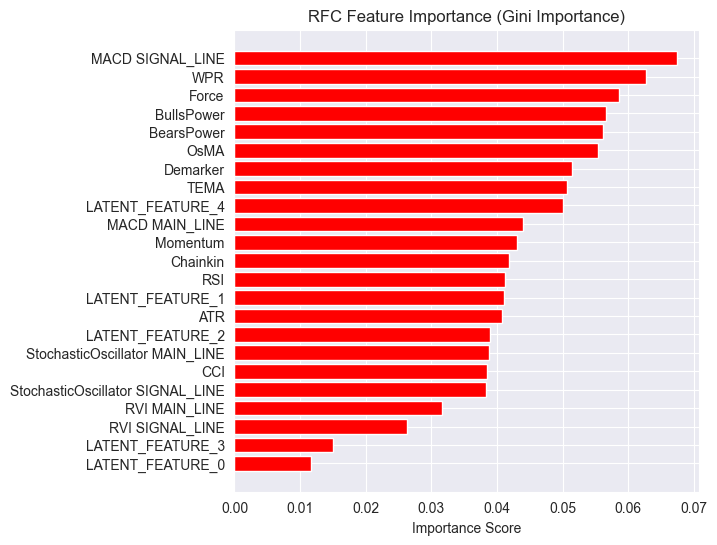
潜在特征被证明对模型很重要,这意味着它们携带了一些模式和信息,有助于模型进行预测。
这个模型表现不佳的原因可能在于所使用的目标变量。设定1根K线的“前瞻值”可能是错误的。
在使用这些指标进行交易决策时,我们通常不会用它们来预测下一个周期(bar)的走势。例如,如果 RSI 指标值低于 30(超卖)的阈值,我们可以说市场可能会在未来连续几个周期内呈现看涨趋势。而不是仅仅预测下一根K线,而我们目前训练模型的方式正是这样。
因此,让我们使用 5 个周期的“前瞻值”来重新创建目标变量。
lookahead = 5

df["future_close"] = df["Close"].shift(-lookahead)
new_df = df.dropna()

new_df["Direction"] = np.where(new_df["future_close"]>new_df["Close"], 1, -1) # if a the close value in the next bar(s)=lookahead is above the current close price, thats a long signal otherwise that's a short signal
现在,在训练集和验证集上对模型进行评估,得出了不同的结果。
Train classification report
               precision    recall  f1-score   support

          -1       0.56      0.70      0.62      1706
           1       0.69      0.54      0.61      2050

    accuracy                           0.61      3756
   macro avg       0.62      0.62      0.61      3756
weighted avg       0.63      0.61      0.61      3756

Test classification report
               precision    recall  f1-score   support

          -1       0.46      0.61      0.52       392
           1       0.63      0.48      0.55       548

    accuracy                           0.54       940
   macro avg       0.55      0.55      0.53       940
weighted avg       0.56      0.54      0.54       940
而现在的特征重要性图也有所不同。
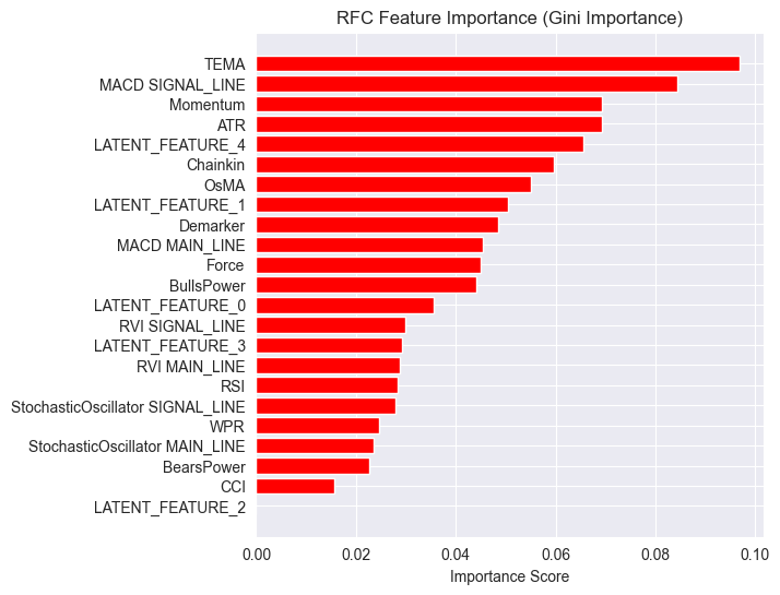
该模型的整体准确率为54%,虽然不算高,但还算过得去,足以让我们相信在特征重要性图上看到的内容。
LGMM生成的一些潜在特征(Latent Features)在模型最具预测性的特征排名中名列前茅。
其中,LATENT_FEATURE_4 成为了随机森林分类器(Random Forest Classifier)的第五大重要特征,其余的潜在特征如 LATENT_FEATURE_0 和 LATENT_FEATURE_1 表现也相当不错,甚至超越了一些原始指标(Raw Indicators)。
总体而言,LGMM生成的大多数特征都包含对分类模型有益的模式。
基于这些信息,你现在已具备理解该指标的基础。
颜色的排列方式类似于潜在特征的排列。
基于LGMM的交易机器人
在EA内部,我们首先导入必要的库文件。
文件名:LGMM BASED EA.mq5
#include <Random Forest.mqh>
#include <Arrays\ArrayString.mqh>
#include <pandas.mqh> //https://www.mql5.com/en/articles/17030
#include <Trade\Trade.mqh>
#include <Trade\PositionInfo.mqh>
#include <Trade\SymbolInfo.mqh>
#include <errordescription.mqh>

CSymbolInfo m_symbol;
CTrade m_trade;
CPositionInfo m_position;
CRandomForestClassifier rfc;
同样,我们必须确保所使用的交易品种和时间周期与训练数据中使用的保持一致。
#define MAGICNUMBER 11062025

input string SYMBOL = "XAUUSD";
input ENUM_TIMEFRAMES TIMEFRAME = PERIOD_D1;
input uint LOOKAHEAD = 5;
input uint SLIPPAGE = 100;
我们在 OnInit 函数中初始化两个模型,即 LGMM 和随机森林分类器模型。
int OnInit()
  {

   if (!MQLInfoInteger(MQL_DEBUG) && !MQLInfoInteger(MQL_TESTER))
    {
      ChartSetSymbolPeriod(0, SYMBOL, TIMEFRAME);
      if (!SymbolSelect(SYMBOL, true))
         {
            printf("%s failed to select SYMBOL %s, Error = %s",__FUNCTION__,SYMBOL,ErrorDescription(GetLastError()));
            return INIT_FAILED;
         }
    }

//--- Loading the Gaussian Mixture model

   string filename = StringFormat("LGMM.%s.%s.onnx",SYMBOL, EnumToString(TIMEFRAME));
   if (!lgmm.Init(filename, ONNX_COMMON_FOLDER))
      {
         printf("%s Failed to initialize the GaussianMixture model (LGMM) in ONNX format file={%s}, Error = %s",__FUNCTION__,filename,ErrorDescription(GetLastError()));
      }

//--- Loading the RFC model

   filename = StringFormat("rfc.%s.%s.onnx",SYMBOL,EnumToString(TIMEFRAME));
   Print(filename);
   if (!rfc.Init(filename, ONNX_COMMON_FOLDER))
      {
         printf("func=%s line=%d, Failed to Load the RFC in ONNX file={%s}, Error = %s",__FUNCTION__,__LINE__,filename,ErrorDescription(GetLastError()));
         return INIT_FAILED;
      }
//...
//... other lines of code
//...
}
在 getX 函数中,我们调用 LGMM 来生成潜在特征,这些特征将与指标数据结合,作为随机森林分类器模型的最终输入。
vector getX(uint start=0, uint count=10)
 {
//--- Get buffers

   CDataFrame df;
   for (uint ind=0; ind<indicators.Size(); ind++) //Loop through all the indicators
      {
        uint buffers_total = indicators[ind].buffer_names.Total();

         for (uint buffer_no=0; buffer_no<buffers_total; buffer_no++) //Their buffer names resemble their buffer numbers
            {
               string name = indicators[ind].buffer_names.At(buffer_no); //Get the name of the buffer, it is helpful for the DataFrame and CSV file

               vector buffer = {};
               if (!buffer.CopyIndicatorBuffer(indicators[ind].handle, buffer_no, start, count)) //Copy indicator buffer
                  {
                     printf("func=%s line=%d | Failed to copy %s indicator buffer, Error = %d",__FUNCTION__,__LINE__,name,GetLastError());
                     continue;
                  }

               df.insert(name, buffer); //Insert a buffer vector and its name to a dataframe object
            }
      }

   if ((uint)df.shape()[0]==0)
      return vector::Zeros(0);

//--- predict the latent features

   vector indicators_data = df.iloc(-1); //index=-1 returns the last row from the dataframe which is the most recent buffer from all indicators

//--- Given the indicators let's predict the latent features

   vector latent_features = lgmm.predict(indicators_data).proba;

   if (latent_features.Size()==0)
      return vector::Zeros(0);

   return hstack(indicators_data, latent_features); //Return indicators data stacked alongside latent features
 }
最后,我们制定了一个简单的交易策略,该策略依赖于随机森林分类器模型产生的交易信号。
void OnTick()
  {
//--- Close trades after AI predictive horizon is over

   CloseTradeAfterTime(MAGICNUMBER, PeriodSeconds(TIMEFRAME)*LOOKAHEAD);

//--- Refresh tick information

   if (!m_symbol.RefreshRates())
     {
       printf("func=%s line=%s. Failed to copy rates, Error = %s",__FUNCTION__,ErrorDescription(GetLastError()));
       return;
     }

//---

    vector x = getX(); //Get all the input for the model

    if (x.Size()==0)
      return;

    long signal = rfc.predict(x).cls; //the class predicted by the random forest classifier
    double proba = rfc.predict(x).proba; //probability of the predictions

    double volume = m_symbol.LotsMin();

    if (!PosExists(POSITION_TYPE_SELL, MAGICNUMBER) && !PosExists(POSITION_TYPE_BUY, MAGICNUMBER)) //no position is open
      {
        if (signal == 1) //If a model predicts a bullish signal
          m_trade.Buy(volume, SYMBOL, m_symbol.Ask()); //Open a buy trade
        else if (signal == -1) // if a model predicts a bearish signal
          m_trade.Sell(volume, SYMBOL, m_symbol.Bid()); //open a sell trade
      }
  }
在模型训练所使用的时间周期上,当经过与“前瞻值(LOOKAHEAD)”相同数量的K线后,我们将平仓。LOOKAHEAD 的值必须与训练脚本中用于构建目标变量时所使用的值保持一致。
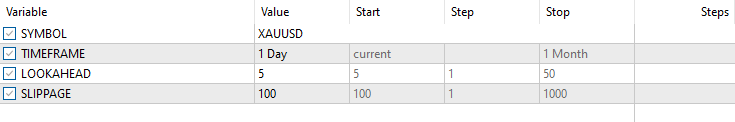
测试器配置。
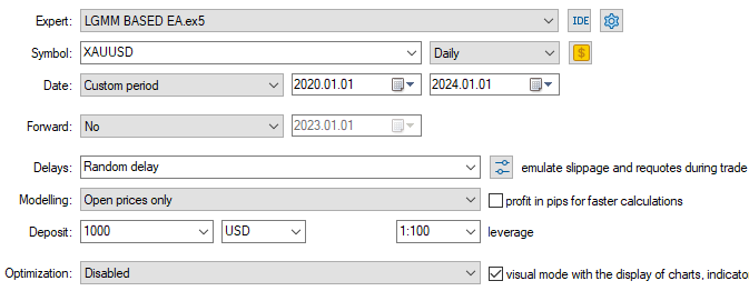
输入
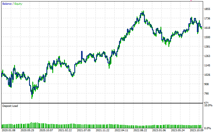
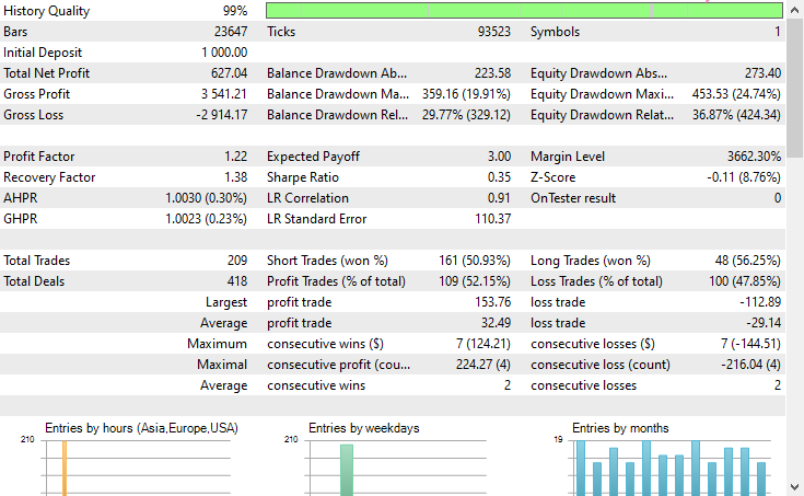
测试器输出
结论
潜在高斯混合模型(LGMM)是一种不错的技术,它能为我们提取出有意义的特征。这些特征包含了不可观测的模式,通常对机器学习模型很有用。然而,与其他任何机器学习模型和预测技术一样,它也存在一些缺点。
潜在高斯混合模型(LGMM):概述
| 因素 | 说明 |
|---|---|
| 什么是 LGMM | 一种提取代表数据中不可观测模式的潜在(隐藏)特征的方法。这些特征对机器学习模型很有用。 |
| 主要优势 | 捕捉数据中有意义的隐藏结构,从而提高模型性能。 |
LGMM 的局限性
| 局限性 | 阐释 |
|---|---|
| 假设高斯分布 | LGMM 假设每个数据点都遵循多元正态分布,而这在往往具有混沌和非线性特征的金融数据中很少见。 |
| 对初始化敏感 | 该模型需要仔细选择分量的数量。初始化不当或参数选择错误会显著降低其有效性。 |
| 结果难以解释 | 它生成的潜在特征难以理解或解释。作为一种无监督方法,它不会对检测到的模式进行标记,只会将它们聚类。 |
| 对异常值敏感 | 高斯分布对异常值不具备鲁棒性。少数极端值可能会扭曲均值并夸大方差,从而扭曲模型的结果。 |
该模型在降维(将大量特征减少为少数几个有意义的特征)以及引入新特征以用更多信息丰富模型方面最为有用。我认为最好以这种方式使用它。
此致敬礼。
欢迎持续关注,并欢迎在这个 GitHub 仓库中为 MQL5 语言的机器学习算法开发做出贡献。
附件表格
| 文件名 | 说明和用法 |
|---|---|
| Include\errordescription.mqh | 包含 MQL5 语言中 MetaTrader 5 平台所产生的所有错误代码说明。 |
| Include\Gaussian Mixture.mqh | 一个包含相关类的库,用于初始化和部署以 ONNX 格式存储的高斯混合模型。 |
| Include\pandas.mqh | 包含一个数据操作类,其功能类似于 Python 编程语言中提供的 Pandas 库,用于数据的存储与处理。 |
| Include\Random Forest.mqh | 一个包含相关类的库,用于初始化和部署以 ONNX 格式存储的随机森林分类器。 |
| Indicators\LGMM Indicator.mq5 | 一个自定义指标,用于显示由潜在高斯混合模型(LGMM)生成的潜在特征。 |
| Scripts\Get XAUUSD Data.mq5 | 一个脚本,用于从 MetaTrader 5 中收集振荡器指标及 OHLCT(开盘价、最高价、最低价、收盘价、时间)数据,并将其保存至 CSV 文件中。 |
| Experts\LGMM BASED EA.mq5 | 利用 LGMM 生成的潜在特征与振荡器指标相结合的组合作为数据输入的EA,根据随机森林分类器提供的预测结果来进行开仓和平仓操作。 |
| Python Code\main.ipynb | 一个 Jupyter 笔记本(Python 脚本),用于数据分析、机器学习模型训练等工作。 |
| Python Code\Trade\TerminalInfo.py | 该文件包含一个类,其功能类似于 MQL5 中提供的 CTerminalInfo,用于获取所选 MetaTrader 5 桌面客户端的相关信息。 |
| Python\requirements.txt | 包含本项目中使用的所有 Python 依赖库及其版本号。 |
| Common\Files\* | 包含一个存有训练数据的示例 CSV 文件,以及本文使用的几个 ONNX 模型文件,仅供学习参考。 |
本文由MetaQuotes Ltd译自英文
原文地址: https://www.mql5.com/en/articles/18497
注意: MetaQuotes Ltd.将保留所有关于这些材料的权利。全部或部分复制或者转载这些材料将被禁止。
本文由网站的一位用户撰写,反映了他们的个人观点。MetaQuotes Ltd 不对所提供信息的准确性负责,也不对因使用所述解决方案、策略或建议而产生的任何后果负责。


 新手在交易中的10个基本错误