

数据科学与机器学习(第四十六部分):在Python中使用N-BEATS进行股票市场预测
 221
221
 1
1

内容
- 什么是N-BEATS模型
- N-BEATS模型的原理简述
- N-BEATS模型的核心设计目标
- 搭建N-BEATS模型
- 基于N-BEATS模型的样本外预测
- 多序列预测
- 在MetaTrader 5中借助N-BEATS模型制定交易决策
- 结论
什么是N-BEATS模型
N-BEATS(基于基函数扩展分析的时间序列预测神经网络)是一种专为时间序列预测设计的深度学习模型。它为单变量和多变量预测任务提供了灵活的框架。
该模型由研究人员Element AI(现已并入ServiceNow)于2019年提出,相关论文为N-BEATS:用于可解释时间序列预测的神经基展开分析。
Element AI的研发团队设计这一模型,旨在打破ARIMA和ETS等经典统计模型在时间序列领域的主导地位,同时兼顾传统机器学习模型所提供的能力。
众所周知,时间序列预测是一项极具挑战性的任务。因此机器学习领域的研究者与从业者常会选用RNNs(循环神经网络)、LSTMs(长短期记忆网络)等深度学习模型,但这类模型普遍存在以下问题:
- 针对简单预测任务而言结构过于繁杂;
- 模型可解释性差;
- 结构虽复杂,性能却未必能稳定超越传统的统计基准模型。
与此同时,ARIMA等传统时间序列预测模型面对大量复杂任务时,建模能力又显得不足。
为此,论文作者与研发团队设计了一款全新时间序列预测深度学习模型,兼顾预测效果、模型可解释性,且无需针对特定业务场景做大量调参优化。

N-BEATS模型的核心设计目标
研发团队在设计该模型时有着清晰的目标与出发点,旨在同时解决传统统计时间序列模型与深度学习时间序列模型各自存在的缺陷。
有关N-BEATS的核心设计目标的详细阐述如下:
- 在保证预测精度的前提下简化模型结构
ARIMA等简单线性时间序列模型难以捕捉数据中的复杂关联特征,而神经网络类深度学习模型却擅长挖掘这类非线性关系。基于此,研发团队选择多层感知机(MLP)这种较为简单的神经网络架构搭建时间序列预测模型,其优势在于可解释性更强、运算速度更快、问题调试更便捷。
如果采用RNN、LSTM、Transformer等深度学习模型,会大幅提升整体系统复杂度,不仅调参难度加大,模型训练速度也会显著变慢。 - 结构可解释性
由于MLP及其他基于神经网络的模型通常难以提供可解释的结果,研究团队旨在构建一种具备可解释预测能力的神经网络模型。该模型借鉴ETS等经典时间序列模型的思路,将预测输出拆解为趋势分量与季节分量。
N-BEATS能够较清晰地对预测结果进行归因,例如判断“这一峰值来自趋势变化”或“这一下降具有季节性”。该特性依托基展开层(多项式基、傅里叶基等)实现。 - 无需领域特定调整的优异精度
本模型的另一核心目标是构建通用时间序列预测模型,可适配各类时间序列数据,且无需复杂的人工特征工程。
Prophet等传统模型需要人工预先指定趋势与季节模式。
N-BEATS可直接从数据中自动学习时序规律。 - 支持多序列全局建模
许多时间序列模型往往一次只处理单条序列,而N‑BEATS可用于多序列(面板数据)预测。该特性在金融场景中实用性极强,可同时预测多个指标。例如同步预测纳斯达克指数和标普500指数的收盘价。
- 训练快速且可扩展性强
相较于循环神经网络、注意力机制模型,N-BEATS训练速度更快、并行拓展性更强。 - 优异的基准性能
通过严谨的回测验证,N-BEATS性能优于ARIMA、ETS等先进的经典时间序列方法。 - 模块化且可拓展的架构设计
传统时间序列模型结构固定、无法自定义修改。N-BEATS采用高灵活模块化架构,可自由新增自定义模块,如趋势模块、季节模块、通用特征模块等。
在正式部署模型前,我们先简要地解析其核心原理。
N-BEATS模型的工作原理(简易数学原理解析)
让我们看一下N-BEATS模型的整体架构。
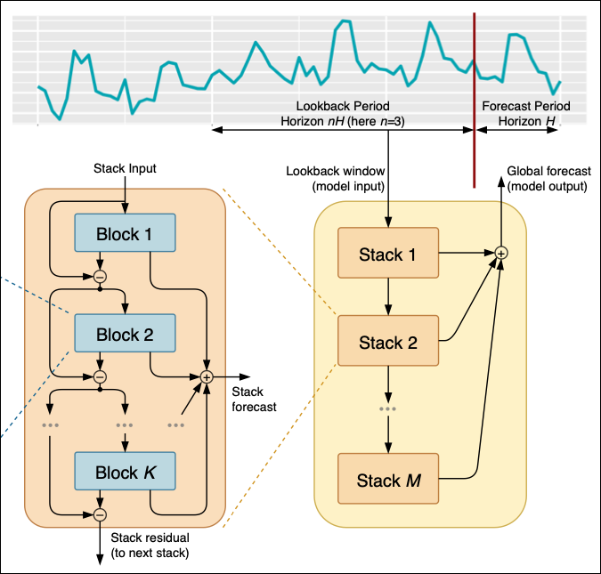
图例01
模型顶层输入为时间序列数据,该数据经过筛选处理后,被送入M个堆叠层(stack)依次运算。
每一个堆叠层由K个网络模块(block)构成。每个模块会输出一组预测值与残差,随后将结果传递至下一层堆叠层继续迭代优化。
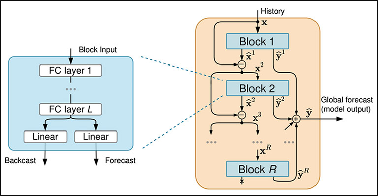
图例02
每个网络模块均包含四层全连接神经网络,可输出回溯重构值或未来预测值。
模型数据流转机制
01:堆叠层机制
模型运行前需预先设定两个核心参数:回溯窗口与预测窗口。
其中,回溯窗口表示向过去回看多长时间,预测窗口表示向未来预测多长时间。
参数设定完成后,第一层堆叠层(Stack 01)读取回溯窗口内的历史数据,完成初始预测。例如,如果回溯窗口为某金融标的近24小时收盘价数据,第一层堆叠层将基于该数据预测未来24小时的价格走势。
初始预测结果与对应的残差(真实值与预测值的差值)会被传递至下一层堆叠层(Stack 02),进行精细化修正。
该迭代优化过程会持续至第M层堆叠层,每一层堆叠层都会在前序预测结果的基础上持续优化精度。
最终,模型整合所有堆叠层的预测结果,输出全局最优预测值。例如,第一层堆叠层捕捉数据峰值波动,第二层修正趋势偏差,最后一层优化长期时序规律,通过将多维度结果融合后,实现高精度预测。
各堆叠层可理解为多维度的数据分析层级:第一层堆叠层擅长捕捉小时级价格波动等短期时序特征,后续堆叠层侧重挖掘日线走势等长期时序规律,
各层分别贡献不同的信息,共同形成最终预测结果。
02:模块内部运行逻辑
首个模块(Block 01)接收堆叠层输入数据(原始回溯数据或上一层堆叠层的残差数据),同时生成回溯重构值与未来预测值。例如,如果模块输入为过去24小时的电力消耗数据,将同步输出未来24小时的消耗预测值与原始输入数据的回溯重构值。
回溯重构值能够帮助模型优化残差特征,提升后续预测的精准度。
同一堆叠层内的多个模块按顺序迭代运算:首个模块输出残差与预测结果后,下一个模块会同时接收前序模块残差与原始堆叠层输入数据双输入特征。双输入机制让后续模块在迭代优化时,既保留原始数据特征,又修正前序预测误差,逐步提升预测精度。
堆叠层内的逐层迭代优化,确保预测结果精度持续提升。当单个堆叠层内所有模块运算完成后,最后一个模块(Block K)输出的最终残差,将传递至下一层堆叠层,开启新一轮优化。
03: 模块结构解析
每个独立的模块均配置四层全连接神经网络,负责完成数据变换与特征提取,为回溯重构与时间序列预测提供特征支撑。
模块内的全连接层完成数据处理与特征提取后,会将特征信息分流为两支(详见图例02) :一支用于生成回溯重构值,另一支用于生成未来预测值。
回溯重构值用于拟合还原原始输入数据,优化残差传递效果;预测值则输出预测窗口内的最终时间序列预测结果。
在Python中搭建N-BEATS模型
首先安装附件中requirements.txt文件内的全部依赖库(附件在文章末尾),安装指令如下:
pip install -r requirements.txt
在 test.ipynb文件中,导入所有所需的模块。
import MetaTrader5 as mt5
import numpy as np
import matplotlib.pyplot as plt
import pandas as pd
import seaborn as sns
import warnings

sns.set_style("darkgrid")
warnings.filterwarnings("ignore")
接着初始化MetaTrader 5:
if not mt5.initialize():
    print("Metratrader5 initialization failed, Error code =", mt5.last_error())
    mt5.shutdown()
我们从纳斯达克指数(NAS100)的日线周期获取1000根K线数据:
rates = mt5.copy_rates_from_pos("NAS100", mt5.TIMEFRAME_D1, 1, 1000)
rates_df = pd.DataFrame(rates)
尽管传统机器学习方法通常采用多变量建模技术,N‑BEATS却采用了类似ARIMA和VAR等传统时间序列模型的单变量建模思路。
单变量数据的构建方法如下:
univariate_df = rates_df[["time", "close"]].copy()
univariate_df["ds"] = pd.to_datetime(univariate_df["time"], unit="s") # convert the time column to datetime
univariate_df["y"] = univariate_df["close"] # closing prices
univariate_df["unique_id"] = "NAS100" # add a unique_id column | very important for univariate models

# Final dataframe
univariate_df = univariate_df[["unique_id", "ds", "y"]].copy()

univariate_df
输出:
| unique_id | ds | y | |
|---|---|---|---|
| 0 | NAS100 | 2021-08-30 | 9.655648 |
| 1 | NAS100 | 2021-08-31 | 9.654988 |
| 2 | NAS100 | 2021-09-01 | 9.655763 |
| 3 | NAS100 | 2021-09-02 | 9.654981 |
| 4 | NAS100 | 2021-09-03 | 9.658335 |
| ... | ... | ... | ... |
| 995 | NAS100 | 2025-07-07 | 10.028180 |
| 996 | NAS100 | 2025-07-08 | 10.031142 |
| 997 | NAS100 | 2025-07-09 | 10.037376 |
| 998 | NAS100 | 2025-07-10 | 10.036098 |
| 999 | NAS100 | 2025-07-11 | 10.033283 |
univariate_df["unique_id"] = "NAS100" # add a unique_id column | very important for univariate models
包含N-BEATS模型的neuralforecast 模块,在设计上可同时处理单变量时序与面板数据(多序列)预测。通过unique_id 字段传递给模型每一行数据属于哪一条时间序列。该字段在以下场景中尤为关键:
- 同时对多个资产或品种进行预测(如AAPL、TSLA、MSFT、EURUSD等);
- 希望用批量训练方式,用一个模型拟合多条时间序列。
由于内部存在分组与索引机制,即使只有单条时序,该字段也为必填项。
训练该模型仅需少量代码即可完成。
from neuralforecast import NeuralForecast
from neuralforecast.models import NBEATS # Neural Basis Expansion Analysis for Time Series

# Define model and horizon
horizon = 30  # forecast 30 days into the future

model = NeuralForecast(
    models=[NBEATS(h=horizon, # predictive horizon of the model
                   input_size=90, # considered autorregresive inputs (lags), y=[1,2,3,4] input_size=2 -> lags=[1,2].
                   max_steps=100, # maximum number of training steps (epochs)
                   scaler_type='robust', # scaler type for the time series data
                   )],
    freq='D' # frequency of the time series data
)

# Fit the model
model.fit(df=univariate_df)
输出:
Seed set to 1
GPU available: False, used: False
TPU available: False, using: 0 TPU cores
HPU available: False, using: 0 HPUs

  | Name         | Type          | Params | Mode
-------------------------------------------------------
0 | loss         | MAE           | 0      | train
1 | padder_train | ConstantPad1d | 0      | train
2 | scaler       | TemporalNorm  | 0      | train
3 | blocks       | ModuleList    | 2.6 M  | train
-------------------------------------------------------
2.6 M     Trainable params
7.3 K     Non-trainable params
2.6 M     Total params
10.541    Total estimated model params size (MB)
31        Modules in train mode
0         Modules in eval mode

Epoch 99: 100%
 1/1 [00:01<00:00,  0.88it/s, v_num=32, train_loss_step=0.259, train_loss_epoch=0.259]
`Trainer.fit` stopped: `max_steps=100` reached.
我们可以在同一坐标系中可视化展示预测值与真实值。
forecast = model.predict() # predict future values based on the fitted model

# Merge forecast with original data
plot_df = pd.merge(univariate_df, forecast, on='ds', how='outer')

plt.figure(figsize=(7,5))
plt.plot(plot_df['ds'], plot_df['y'], label='Actual')
plt.plot(plot_df['ds'], plot_df['NBEATS'], label='Forecast')
plt.axvline(plot_df['ds'].max() - pd.Timedelta(days=horizon), color='gray', linestyle='--')
plt.legend()
plt.title('N-BEATS Forecast')
plt.show()
输出:
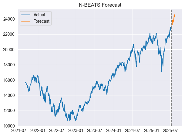
合并后数据框的展示效果如下:
| unique_id_x | ds | y | unique_id_y | NBEATS | |
|---|---|---|---|---|---|
| 0 | NAS100 | 2021-08-31 | 15599.4 | NaN | NaN |
| 1 | NAS100 | 2021-09-01 | 15611.5 | NaN | NaN |
| 2 | NAS100 | 2021-09-02 | 15599.3 | NaN | NaN |
| 3 | NAS100 | 2021-09-03 | 15651.7 | NaN | NaN |
| 4 | NAS100 | 2021-09-06 | 15700.4 | NaN | NaN |
| ... | ... | ... | ... | ... | ... |
| 1025 | NaN | 2025-08-09 | NaN | NAS100 | 24235.187500 |
| 1026 | NaN | 2025-08-10 | NaN | NAS100 | 24466.316406 |
| 1027 | NaN | 2025-08-11 | NaN | NAS100 | 24454.646484 |
| 1028 | NaN | 2025-08-12 | NaN | NAS100 | 24405.820312 |
| 1029 | NaN | 2025-08-13 | NaN | NAS100 | 24571.919922 |
非常棒,模型已完成未来30天的预测。
为进行模型评估,我们按照常规机器学习模型的验证方式,在一个数据集上训练,在另一个数据集上测试。
基于N-BEATS模型的样本外预测
首先将数据划分为训练集与测试集。
split_date = '2024-01-01'  # the split date for training and testing

train_df = univariate_df[univariate_df['ds'] < split_date]
test_df = univariate_df[univariate_df['ds'] >= split_date]
我们在训练集上对模型进行训练。
model = NeuralForecast(
    models=[NBEATS(h=horizon, # predictive horizon of the model
                   input_size=90, # considered autorregresive inputs (lags), y=[1,2,3,4] input_size=2 -> lags=[1,2].
                   max_steps=100, # maximum number of training steps (epochs)
                   scaler_type='robust', # scaler type for the time series data
                   )],
    freq='D' # frequency of the time series data
)

# Fit the model
model.fit(df=train_df)
由于预测函数会根据预测步长直接预测未来N天的数据,因此为了评估模型的样本外预测效果,我们需要将预测结果与真实值数据框进行合并。
test_forecast = model.predict() # predict future 30 days based on the training data

df_test = pd.merge(test_df, test_forecast, on=['ds', 'unique_id'], how='outer') # merge the test data with the forecast
df_test.dropna(inplace=True) # drop rows with NaN values

df_test
输出:
| unique_id | ds | y | NBEATS | |
|---|---|---|---|---|
| 3 | NAS100 | 2024-01-02 | 16554.3 | 16569.835938 |
| 4 | NAS100 | 2024-01-03 | 16368.1 | 16596.839844 |
| 5 | NAS100 | 2024-01-04 | 16287.2 | 16603.513672 |
| 6 | NAS100 | 2024-01-05 | 16307.1 | 16729.607422 |
| 9 | NAS100 | 2024-01-08 | 16631.0 | 16854.746094 |
| 10 | NAS100 | 2024-01-09 | 16672.4 | 16918.466797 |
| 11 | NAS100 | 2024-01-10 | 16804.7 | 16958.833984 |
| 12 | NAS100 | 2024-01-11 | 16814.3 | 17130.972656 |
| 13 | NAS100 | 2024-01-12 | 16808.8 | 17055.396484 |
| 16 | NAS100 | 2024-01-15 | 16828.7 | 17272.376953 |
| 17 | NAS100 | 2024-01-16 | 16841.9 | 17227.498047 |
| 18 | NAS100 | 2024-01-17 | 16727.7 | 17408.158203 |
| 19 | NAS100 | 2024-01-18 | 16987.0 | 17499.619141 |
| 20 | NAS100 | 2024-01-19 | 17336.7 | 17318.767578 |
| 23 | NAS100 | 2024-01-22 | 17329.3 | 17399.562500 |
| 24 | NAS100 | 2024-01-23 | 17426.1 | 17289.140625 |
| 25 | NAS100 | 2024-01-24 | 17503.1 | 17236.478516 |
| 26 | NAS100 | 2024-01-25 | 17469.4 | 17188.691406 |
| 27 | NAS100 | 2024-01-26 | 17390.1 | 17315.134766 |
我们继续对预测结果进行评估。
from sklearn.metrics import mean_absolute_percentage_error, r2_score

mape = mean_absolute_percentage_error(df_test['y'], df_test['NBEATS'])
r2_score_ = r2_score(df_test['y'], df_test['NBEATS'])

print(f"mean_absolute_percentage_error (MAPE): {mape} \n R2 Score: {r2_score_}")
输出:
mean_absolute_percentage_error (MAPE): 0.015779373328172166
R2 Score: 0.35350182943487285
从MAPE(平均绝对百分比误差)指标来看,模型预测的百分比精度很高;但R²得分为0.35,说明模型仅能解释目标变量35%的波动。
真实值与预测值在同一坐标系下的对比图如下:
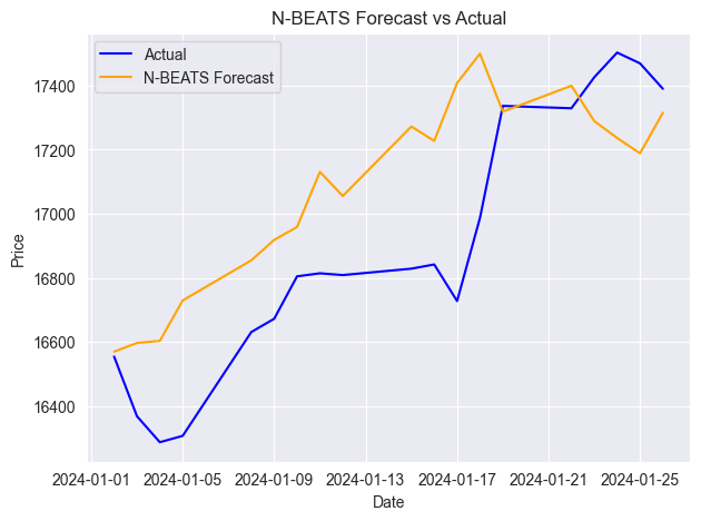
与其他时间序列预测模型一样,N-BEATS也需要定期用新的时序数据更新,才能保持预测的时效性与准确性。在之前的示例中,我们基于日线数据一次性预测未来30天并进行评估,但这种方式并不合理,因为模型会遗漏期间大量的每日信息。
正确的做法是:一旦有新数据产生,就立即用新数据更新模型。
N-BEATS模型提供了非常简便的方式,无需重新训练即可用新数据更新模型,大幅节省时间。
当您执行:
NBEATS.predict(df=new_dataframe) 模型会在保持已训练权重不变的情况下,对新数据进行推理,从而基于最新输入给出更新后的预测结果。
多序列预测
正如之前N-BEATS核心目标部分所述,该模型在设计上就非常擅长处理多序列预测任务。
这正是它的一大亮点,因为模型能把从一条时间序列学到的规律迁移应用,从而提升多条序列的整体预测效果。
该功能的使用方法如下:
我们首先从MetaTrader 5中分别获取各品种的数据:
rates_nq = mt5.copy_rates_from_pos("NAS100", mt5.TIMEFRAME_D1, 1, 1000)
rates_df_nq = pd.DataFrame(rates_nq)

rates_snp = mt5.copy_rates_from_pos("US500", mt5.TIMEFRAME_D1, 1, 1000)
rates_df_snp = pd.DataFrame(rates_snp)
再分别构建各自的单变量数据框。
# NAS100
rates_df_nq["ds"] = pd.to_datetime(rates_df_nq["time"], unit="s")
rates_df_nq["y"] = rates_df_nq["close"]
rates_df_nq["unique_id"] = "NAS100"
df_nq = rates_df_nq[["unique_id", "ds", "y"]]

# US500
rates_df_snp["ds"] = pd.to_datetime(rates_df_snp["time"], unit="s")
rates_df_snp["y"] = rates_df_snp["close"]
rates_df_snp["unique_id"] = "US500"
df_snp = rates_df_snp[["unique_id", "ds", "y"]]
我们将两个数据框合并,并按照日期列ds和unique_id对数据进行排序。
multivariate_df = pd.concat([df_nq, df_snp], ignore_index=True) # combine both dataframes
multivariate_df = multivariate_df.sort_values(['unique_id', 'ds']).reset_index(drop=True) # sort by unique_id and date

multivariate_df
输出:
| unique_id | ds | y | |
|---|---|---|---|
| 0 | NAS100 | 2021-08-31 | 15599.4 |
| 1 | NAS100 | 2021-09-01 | 15611.5 |
| 2 | NAS100 | 2021-09-02 | 15599.3 |
| 3 | NAS100 | 2021-09-03 | 15651.7 |
| 4 | NAS100 | 2021-09-06 | 15700.4 |
| ... | ... | ... | ... |
| 1995 | US500 | 2025-07-08 | 6229.9 |
| 1996 | US500 | 2025-07-09 | 6264.9 |
| 1997 | US500 | 2025-07-10 | 6280.3 |
| 1998 | US500 | 2025-07-11 | 6255.8 |
| 1999 | US500 | 2025-07-14 | 6271.9 |
和之前的操作相同,我们将数据划分为训练集和测试集。
split_date = '2024-01-01'  # the split date for training and testing

train_df = multivariate_df[multivariate_df['ds'] < split_date]
test_df = multivariate_df[multivariate_df['ds'] >= split_date]
接下来,我们使用和之前完全相同的方式训练模型。
from neuralforecast import NeuralForecast
from neuralforecast.models import NBEATS # Neural Basis Expansion Analysis for Time Series

# Define model and horizon
horizon = 30  # forecast 30 days into the future

model = NeuralForecast(
    models=[NBEATS(h=horizon, # predictive horizon of the model
                   input_size=90, # considered autorregresive inputs (lags), y=[1,2,3,4] input_size=2 -> lags=[1,2].
                   max_steps=100, # maximum number of training steps (epochs)
                   scaler_type='robust', # scaler type for the time series data
                   )],
    freq='D' # frequency of the time series data
)

# Fit the model
model.fit(df=train_df)
我们对样本外数据进行预测。
test_forecast = model.predict() # predict future 30 days based on the training data

df_test = pd.merge(test_df, test_forecast, on=['ds', 'unique_id'], how='outer') # merge the test data with the forecast
df_test.dropna(inplace=True) # drop rows with NaN values

df_test
输出:
| unique_id | ds | y | NBEATS | |
|---|---|---|---|---|
| 6 | NAS100 | 2024-01-02 | 16554.3 | 16267.765625 |
| 7 | US500 | 2024-01-02 | 4747.4 | 4706.230957 |
| 8 | NAS100 | 2024-01-03 | 16368.1 | 16230.808594 |
| 9 | US500 | 2024-01-03 | 4707.3 | 4706.517090 |
| 10 | NAS100 | 2024-01-04 | 16287.2 | 16136.568359 |
| 11 | US500 | 2024-01-04 | 4690.9 | 4686.380859 |
| 12 | NAS100 | 2024-01-05 | 16307.1 | 16218.930664 |
| 13 | US500 | 2024-01-05 | 4695.8 | 4704.896484 |
最后,我们对两个交易品种分别进行模型评估,并在同一坐标系中可视化展示真实值与预测值。
from sklearn.metrics import mean_absolute_percentage_error, r2_score

unique_ids = df_test['unique_id'].unique()

for unique_id in unique_ids:

    df_unique = df_test[df_test['unique_id'] == unique_id].copy()

    mape = mean_absolute_percentage_error(df_unique['y'], df_unique['NBEATS'])
    r2_score_ = r2_score(df_unique['y'], df_unique['NBEATS'])


    print(f"Unique ID: {unique_id} - MAPE: {mape}, R2 Score: {r2_score_}")


    plt.figure(figsize=(7, 4))
    plt.plot(df_unique['ds'], df_unique['y'], label='Actual', color='blue')
    plt.plot(df_unique['ds'], df_unique['NBEATS'], label='Forecast', color='orange')
    plt.title(f'Actual vs Forecast for {unique_id}')
    plt.xlabel('Date')
    plt.ylabel('Value')
    plt.legend()
    plt.show()
输出:
Unique ID: NAS100 - MAPE: 0.0221775184381915, R2 Score: -0.16976266747298419

Unique ID: US500 - MAPE: 0.007412931117247571, R2 Score: 0.3782229067061038

在MetaTrader 5中借助N-BEATS模型制定交易决策
现在,我们已经可以通过该模型获取预测结果,接下来可以将模型集成到基于Python开发的交易机器人中。
在文件NBEATS-tradingbot.py中,我们首先编写用于完整初始化训练模型的函数:
def train_nbeats_model(forecast_horizon: int=30,
                       start_bar: int=1,
                       number_of_bars: int=1000,
                       input_size: int=90,
                       max_steps: int=100,
                       mt5_timeframe: int=mt5.TIMEFRAME_D1,
                       symbol_01: str="NAS100",
                       symbol_02: str="US500",
                       test_size_percentage: float=0.2,
                       scaler_type: str='robust'):

    """
        Train NBEATS model on NAS100 and US500 data from MetaTrader 5.

        Args:
            start_bar: starting bar to be used to in CopyRates from MT5
            number_of_bars: The number of bars to extract from MT5 for training the model
            forecast_horizon: the number of days to predict in the future
            input_size: number of previous days to consider for prediction
            max_steps: maximum number of training steps (epochs)
            mt5_timeframe: timeframe to be used for the data extraction from MT5
            symbol_01: unique identifier for the first symbol (default is NAS100)
            symbol_02: unique identifier for the second symbol (default is US500)
            test_size_percentage: percentage of the data to be used for testing (default is 0.2)
            scaler_type: type of scaler to be used for the time series data (default is 'robust')

        Returns:
            NBEATS: the n-beats model object
    """

    # Getting data from MetaTrader 5

    rates_nq = mt5.copy_rates_from_pos(symbol_01, mt5_timeframe, start_bar, number_of_bars)
    rates_df_nq = pd.DataFrame(rates_nq)

    rates_snp = mt5.copy_rates_from_pos(symbol_02, mt5_timeframe, start_bar, number_of_bars)
    rates_df_snp = pd.DataFrame(rates_snp)

    if rates_df_nq.empty or rates_df_snp.empty:
        print(f"Failed to retrieve data for {symbol_01} or {symbol_02}.")
        return None

    # Getting NAS100 data
    rates_df_nq["ds"] = pd.to_datetime(rates_df_nq["time"], unit="s")
    rates_df_nq["y"] = rates_df_nq["close"]
    rates_df_nq["unique_id"] = symbol_01
    df_nq = rates_df_nq[["unique_id", "ds", "y"]]

    # Getting US500 data
    rates_df_snp["ds"] = pd.to_datetime(rates_df_snp["time"], unit="s")
    rates_df_snp["y"] = rates_df_snp["close"]
    rates_df_snp["unique_id"] = symbol_02
    df_snp = rates_df_snp[["unique_id", "ds", "y"]]

    multivariate_df = pd.concat([df_nq, df_snp], ignore_index=True) # combine both dataframes
    multivariate_df = multivariate_df.sort_values(['unique_id', 'ds']).reset_index(drop=True) # sort by unique_id and date

    # Group by unique_id and split per group
    train_df_list = []
    test_df_list = []

    for _, group in multivariate_df.groupby('unique_id'):
        group = group.sort_values('ds')
        split_idx = int(len(group) * (1 - test_size_percentage))

        train_df_list.append(group.iloc[:split_idx])
        test_df_list.append(group.iloc[split_idx:])

    # Concatenate all series
    train_df = pd.concat(train_df_list).reset_index(drop=True)
    test_df = pd.concat(test_df_list).reset_index(drop=True)

    # Define model and horizon

    model = NeuralForecast(
        models=[NBEATS(h=forecast_horizon, # predictive horizon of the model
                    input_size=input_size, # considered autorregresive inputs (lags), y=[1,2,3,4] input_size=2 -> lags=[1,2].
                    max_steps=max_steps, # maximum number of training steps (epochs)
                    scaler_type=scaler_type, # scaler type for the time series data
                    )],
        freq='D' # frequency of the time series data
    )

    # fit the model on the training data

    model.fit(df=train_df)

    test_forecast = model.predict() # predict future 30 days based on the training data

    df_test = pd.merge(test_df, test_forecast, on=['ds', 'unique_id'], how='outer') # merge the test data with the forecast
    df_test.dropna(inplace=True) # drop rows with NaN values


    unique_ids = df_test['unique_id'].unique()
    for unique_id in unique_ids:

        df_unique = df_test[df_test['unique_id'] == unique_id].copy()

        mape = mean_absolute_percentage_error(df_unique['y'], df_unique['NBEATS'])
        print(f"Unique ID: {unique_id} - MAPE: {mape:.2f}")

    return model
该函数整合了前面介绍的全部训练流程,并返回可直接用于预测的N-BEATS模型对象。
用于预测后续数值的函数,其实现方法与训练函数基本一致。
def predict_next(model,
                  symbol_unique_id: str,
                  input_size: int=90):

    """
        Predict the next values for a given unique_id using the trained model.

        Args:
            model (NBEATS): the trained NBEATS model
            symbol_unique_id (str): unique identifier for the symbol to predict
            input_size (int): number of previous days to consider for prediction

        Returns:
            DataFrame: containing the predicted values for the next days
    """

    # Getting data from MetaTrader 5

    rates = mt5.copy_rates_from_pos(symbol_unique_id, mt5.TIMEFRAME_D1, 1, input_size * 2)  # Get enough data for prediction
    if rates is None or len(rates) == 0:
        print(f"Failed to retrieve data for {symbol_unique_id}.")
        return pd.DataFrame()

    rates_df = pd.DataFrame(rates)

    rates_df["ds"] = pd.to_datetime(rates_df["time"], unit="s")
    rates_df = rates_df[["ds", "close"]].rename(columns={"close": "y"})
    rates_df["unique_id"] = symbol_unique_id
    rates_df = rates_df.sort_values(by="ds").reset_index(drop=True)

    # Prepare the dataframe for reference & prediction
    univariate_df = rates_df[["unique_id", "ds", "y"]]
    forecast = model.predict(df=univariate_df)

    return forecast
我们给模型传入的数据长度,设置为训练时input_size的两倍,只为了给模型提供足够的输入数据。
让我们对每个品种分别调用两次预测函数,并观察输出的结果数据框。
trained_model = train_nbeats_model(max_steps=10)

print(predict_next(trained_model, "NAS100").head())
print(predict_next(trained_model, "US500").head())
输出:
Predicting DataLoader 0: 100%|████████████████████████████████████████████████████████████████████████████████████████████████| 1/1 [00:00<00:00, 45.64it/s]
  unique_id         ds        NBEATS
0    NAS100 2025-07-16  22836.160156
1    NAS100 2025-07-17  22931.242188
2    NAS100 2025-07-18  22984.792969
3    NAS100 2025-07-19  23037.224609
4    NAS100 2025-07-20  23119.804688
GPU available: False, used: False
TPU available: False, using: 0 TPU cores
HPU available: False, using: 0 HPUs
Predicting DataLoader 0: 100%|████████████████████████████████████████████████████████████████████████████████████████████████| 1/1 [00:00<00:00, 71.43it/s]
  unique_id         ds       NBEATS
0     US500 2025-07-16  6234.584961
1     US500 2025-07-17  6254.846680
2     US500 2025-07-18  6261.153320
3     US500 2025-07-19  6282.960449
4     US500 2025-07-20  6307.293945
GPU available: False, used: False
TPU available: False, using: 0 TPU cores
HPU available: False, using: 0 HPUs
由于两个品种的结果数据框都包含未来30天的每日收盘价预测(当前日期为2025年7月16日),我们需要从中选取对应今日日期的预测值。
today = dt.datetime.now().date() # today's date

forecast_df = predict_next(trained_model, "NAS100") # Get the predicted values for NAS100, 30 days into the future
today_pred_close_nq = forecast_df[forecast_df['ds'].dt.date == today]['NBEATS'].values # extract today's predicted close value for NAS100

forecast_df = predict_next(trained_model, "US500") # Get the predicted values for US500, 30 days into the future
today_pred_close_snp = forecast_df[forecast_df['ds'].dt.date == today]['NBEATS'].values # extract today's predicted close value for US500

print(f"Today's predicted NAS100 values:", today_pred_close_nq)
print(f"Today's predicted US500 values:", today_pred_close_snp)
输出:
Today's predicted NAS100 values: [22836.16]
Today's predicted US500 values: [6234.585]
最后,我们就可以在一个简易交易策略中使用这些预测值。
# Trading modules

from Trade.Trade import CTrade
from Trade.PositionInfo import CPositionInfo
from Trade.SymbolInfo import CSymbolInfo

SLIPPAGE = 100 # points
MAGIC_NUMBER = 15072025 # unique identifier for the trades
TIMEFRAME = mt5.TIMEFRAME_D1 # timeframe for the trades

# Create trade objects for NAS100 and US500
m_trade_nq = CTrade(magic_number=MAGIC_NUMBER,
                 filling_type_symbol = "NAS100",
                 deviation_points=SLIPPAGE)

m_trade_snp = CTrade(magic_number=MAGIC_NUMBER,
                 filling_type_symbol = "US500",
                 deviation_points=SLIPPAGE)

# Training the NBEATS model INITIALLY
trained_model = train_nbeats_model(max_steps=10,
                                    input_size=90,
                                    forecast_horizon=30,
                                    start_bar=1,
                                    number_of_bars=1000,
                                    mt5_timeframe=TIMEFRAME,
                                    symbol_01="NAS100",
                                    symbol_02="US500"
                                   )

m_symbol_nq = CSymbolInfo("NAS100") # Create symbol info object for NAS100
m_symbol_snp = CSymbolInfo("US500") # Create symbol info object for US500

m_position = CPositionInfo() # Create position info object


def pos_exists(pos_type: int, magic: int, symbol: str) -> bool:

    """ Checks whether a position exists given a magic number, symbol, and the position type

    Returns:
        bool: True if a position is found otherwise False
    """

    if mt5.positions_total() < 1: # no positions whatsoever
        return False

    positions = mt5.positions_get()

    for position in positions:
        if m_position.select_position(position):
            if m_position.magic() == magic and m_position.symbol() == symbol and m_position.position_type()==pos_type:
                return True

    return False


def RunStrategyandML(trained_model: NBEATS):

    today = dt.datetime.now().date() # today's date

    forecast_df = predict_next(trained_model, "NAS100") # Get the predicted values for NAS100, 30 days into the future
    today_pred_close_nq = forecast_df[forecast_df['ds'].dt.date == today]['NBEATS'].values # extract today's predicted close value for NAS100

    forecast_df = predict_next(trained_model, "US500") # Get the predicted values for US500, 30 days into the future
    today_pred_close_snp = forecast_df[forecast_df['ds'].dt.date == today]['NBEATS'].values # extract today's predicted close value for US500

    # convert numpy arrays to float values

    today_pred_close_nq = float(today_pred_close_nq[0]) if len(today_pred_close_nq) > 0 else None
    today_pred_close_snp = float(today_pred_close_snp[0]) if len(today_pred_close_snp) > 0 else None

    print(f"Today's predicted NAS100 values:", today_pred_close_nq)
    print(f"Today's predicted US500 values:", today_pred_close_snp)

    # Refreshing the rates for NAS100 and US500 symbols

    m_symbol_nq.refresh_rates()
    m_symbol_snp.refresh_rates()

    ask_price_nq = m_symbol_nq.ask() # get today's close price for NAS100
    ask_price_snp = m_symbol_snp.ask() # get today's close price for US500

    # Trading operations for the NAS100 symol

    if not pos_exists(pos_type=mt5.ORDER_TYPE_BUY, magic=MAGIC_NUMBER, symbol="NAS100"):
        if today_pred_close_nq > ask_price_nq: # if predicted close price for NAS100 is greater than the current ask price
            # Open a buy trade
            m_trade_nq.buy(volume=m_symbol_nq.lots_min(),
                            symbol="NAS100",
                            price=m_symbol_nq.ask(),
                            sl=0.0,
                            tp=today_pred_close_nq) # set take profit to the predicted close price

    print("ask: ", m_symbol_nq.ask(), "bid: ", m_symbol_nq.bid(), "last: ", ask_price_nq)
    print("tp: ", today_pred_close_nq, "lots: ", m_symbol_nq.lots_min())
    print("istp within range: ", (m_symbol_nq.ask() - today_pred_close_nq) > m_symbol_nq.stops_level())

    if not pos_exists(pos_type=mt5.ORDER_TYPE_SELL, magic=MAGIC_NUMBER, symbol="NAS100"):
        if today_pred_close_nq < ask_price_nq: # if predicted close price for NAS100 is less than the current bid price
            m_trade_nq.sell(volume=m_symbol_nq.lots_min(),
                             symbol="NAS100",
                             price=m_symbol_nq.bid(),
                             sl=0.0,
                             tp=today_pred_close_nq) # set take profit to the predicted close price


    # Buy and sell operations for the US500 symbol


    if not pos_exists(pos_type=mt5.ORDER_TYPE_BUY, magic=MAGIC_NUMBER, symbol="US500"):
        if today_pred_close_snp > ask_price_snp: # if the predicted price for US500 is greater than the current ask price
            m_trade_snp.buy(volume=m_symbol_snp.lots_min(),
                            symbol="US500",
                            price=m_symbol_snp.ask(),
                            sl=0.0,
                            tp=today_pred_close_snp)

    if not pos_exists(pos_type=mt5.ORDER_TYPE_SELL, magic=MAGIC_NUMBER, symbol="US500"):
        if today_pred_close_snp < ask_price_snp: # if the predicted price for US500 is less than the current bid price
            m_trade_snp.sell(volume=m_symbol_snp.lots_min(),
                             symbol="US500",
                             price=m_symbol_snp.bid(),
                             sl=0.0,
                             tp=today_pred_close_snp)


RunStrategyandML(trained_model=trained_model) # Run the strategy and ML model once to initialize
输出:
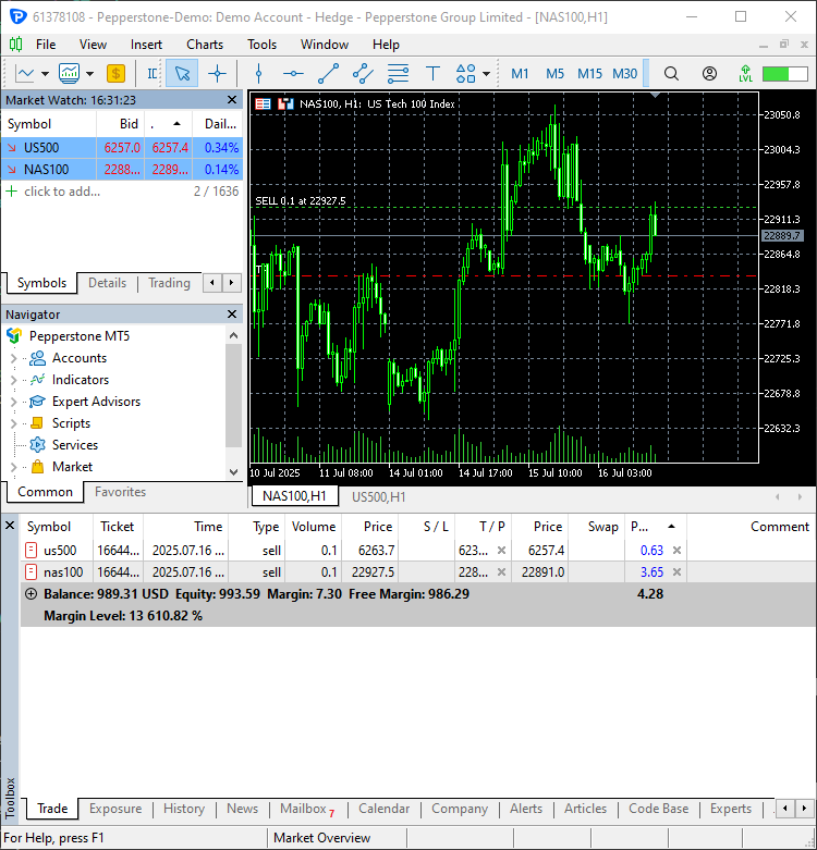
已新开两笔交易。
最后,我们可以对训练过程设置定时任务,让模型自动进行预测,并在每天开始时自动下单。
# Schedule the strategy to run every day at 00:00
schedule.every().day.at("00:00").do(RunStrategyandML, trained_model=trained_model)

while True:

    schedule.run_pending()
    time.sleep(10)
结论
N‑BEATS是一款用于时间序列分析与预测的强大模型。在同类任务中,它的表现优于ARIMA、VAR、Prophet等传统模型,因为其核心基于神经网络,能够出色捕捉复杂数据模式。
对于希望使用非传统时间序列模型进行预测的开发者而言,N‑BEATS是非常理想的选择。
我很欣赏它内置了归一化方法与评估工具,方便模型使用。
尽管该模型表现出色,但和世界上所有机器学习模型一样,也存在一些不容忽视的缺点,其中包括:
- 主要面向单变量预测设计
如之前所述,模型在训练时通常只需要两个特征:ds(时间戳)和目标变量y。这一点与之前探讨的Prophet模型类似。
而在金融数据中,仅靠这两个特征不足以完整刻画市场动态。 - 容易在噪声数据上过拟合
与其他深度网络一样,N‑BEATS在包含大量噪声的数据上容易出现过拟合问题。 - 可解释性有限
虽然N‑BEATS通过基函数分解提供了一定可解释性,但它本质仍是深度神经网络,可解释性远不如ARIMA、Prophet等传统时间序列模型。 - 行业普及度较低
您很可能之前从未听说过此模型。
尽管它在学术基准测试中表现强劲,但与ARIMA、XGBoost、LSTM等模型相比,其在机器学习业界的应用并不广泛,网上相关的教程与文章也相对较少。
谨此结束。
附件表
| 文件名 | 说明/用法 |
|---|---|
| Trade\PositionInfo.py | 包含CPositionInfo 类,功能与MQL5中类似,用于获取MetaTrader 5中所有当前持仓的信息。 |
| Trade\SymbolInfo.py | 包含CSymbolInfo类,功能与MQL5中类似,用于从MetaTrader 5获取所选交易品种的完整信息。 |
| Trade\Trade.py | 包含CTrade类,功能与MQL5中类似,提供在MetaTrader 5中开仓和平仓的交易函数。 |
| error_description.py | 包含将MetaTrader 5错误代码转换为可读文本说明的函数。 |
| NBEATS-Tradingbot.py | 使用N-BEATS模型进行交易决策的Python脚本。 |
| test.ipynb | 用于N-BEATS模型实验与调试的Jupyter笔记本。 |
| requirements.txt | 包含本项目所需的所有Python依赖库。 |
来源与参考文献
本文由MetaQuotes Ltd译自英文
原文地址: https://www.mql5.com/en/articles/18242
注意: MetaQuotes Ltd.将保留所有关于这些材料的权利。全部或部分复制或者转载这些材料将被禁止。
本文由网站的一位用户撰写,反映了他们的个人观点。MetaQuotes Ltd 不对所提供信息的准确性负责,也不对因使用所述解决方案、策略或建议而产生的任何后果负责。

 从基础到中级:函数指针
 您应该了解的MQL5向导技巧(第 75 部分):动量震荡指标与包络线的应用
 您应该了解的MQL5向导技巧(第七十六部分):利用AO形态与包络通道进行监督学习建模
 极值优化(EO)

快来看看这篇新文章:《数据科学与机器学习(第46部分):使用Python中的N-BEATS进行股市预测》。
作者:Omega J Msigwa