データサイエンスとML（第43回）：潜在ガウス混合モデル(LGMM)を用いた指標データにおける隠れパターン検出

内容

• はじめに
• 潜在ガウス混合モデル(LGMM)とは 
• LGMMの数学的背景
• インジケーターのデータでLGMMを学習させる
• LGMMに基づくMQL5インジケーター
• LGMMにおける最適なコンポーネント数の探索
• 潜在ガウス混合モデルと分類器モデルの併用
• LGMMを用いた自動売買ロボット
• 結論

はじめに

私たちトレーダーが利用するほとんどすべての取引戦略は、何らかのパターンの識別と検出に基づいています。私たちはインジケーターでパターンや確認を調べることもありますし、時にはサポートラインやレジスタンスラインのようなオブジェクトや線を描画して、市場の状態を特定します。

パターン検出は金融市場において人間にとっては比較的容易な作業ですが、市場は本質的にノイズが多くカオス的であるため、このプロセスをプログラム化して自動化することは非常に困難です。

一部のトレーダーは、この課題に対して人工知能(AI)や機械学習を活用しています。過去の記事の一つでも議論したように、コンピュータビジョンに基づく技術を用いて画像データを処理し、人間と同じようにパターンを認識させるアプローチです。

本記事では、潜在ガウス混合モデル(LGMM: LatentGaussianMixtureModel)という確率的モデルを取り上げます。このモデルはパターン検出に優れており、インジケーターのデータを与えることで、隠れたパターンを検出し、金融市場における予測の精度を高めることが可能です。

潜在ガウス混合モデル(LGMM)とは

潜在ガウス混合モデルは、データが複数の正規分布（ガウス分布）の混合から生成され、それぞれの分布が潜在（観測されない）変数に関連していると仮定する確率モデルです。

これは、各観測値のクラスタ割り当てを説明する潜在変数を組み込んだ、ガウス混合モデル(GMM)の拡張版です。

潜在ガウスモデルは、データを生成する基礎的なプロセスが直接観測できない場合に使用され、これらのプロセスは正規分布に従うと仮定されます。

「潜在」という部分は、回路内の見えない電気信号のように、システムの挙動に影響を与えるが直接測定できない変数を指します。

金融市場では、これらの潜在変数が、私たちがしばしば誤解したり見逃したりするデータ内の基礎的な取引パターンを表すことがあります。

簡単に言えば、LGMMの基本構造は以下の通りです。

• 潜在変数
  
  観測されない変数で、正規分布に従うと仮定され、観測データに影響を与える基礎的要因を表します。
• 観測値
  
  実際に収集されるデータで、通常は非ガウス分布に従い、潜在変数と既知の関数を通じて関連付けられます。
• パラメータ
  
  潜在変数と観測値の関係を支配する要素で、分布の平均や分散などが含まれます。

LGMMの数学的背景

LGMMは確率的生成モデルであり、その核にはクラスタリング手法があります。主な要素は以下の通りです。

潜在変数

• 直接観測されない変数です
• 各データ点がどのコンポーネント（クラスタ）から生成されたかを表します
• 通常、カテゴリ（離散）分布としてモデル化されます。

混合モデル

データの確率分布は、複数の正規分布の重み付き総和として表されます。

ここで

• は混合係数（コンポーネントの事前確率、）
  
• は平均、共分散のガウス分布
  

潜在変数による表現

直接p(x)をモデル化する代わりに、次のように表現します。

ここで

• 
  
• 
  

このモデルの目標は潜在変数とパラメータを推定することです。 

最も一般的に用いられる推定手法は、EMアルゴリズム（期待値最大化、Expectation-Maximization）です。

LGMMのEMアルゴリズム

EMアルゴリズムは、期待ステップ（Eステップ）と最大化ステップ（Mステップ）の2段階からなります。

ステップ01：期待ステップ（Eステップ）

各データ点が各ガウス分布に属する事後確率を推定します。

ステップ02：最大化ステップ（Mステップ）

Eステップで計算した事後確率を使い、パラメータを更新します。

学習中は、モデルが収束するまでEステップとMステップが繰り返し実行されます。

LGMMは、不確実性を伴うデータのクラスタリング（ソフトクラスタリング）、異常検出、密度推定、音声認識関連タスクなど、実社会の多様な分野で活用されています。

インジケーターのデータでLGMMを学習させる

インジケーターデータの中には、トレーダーとして取引判断を下す際に活用するパターンが存在しています。私たちの目標は、まずLGMMを用いてそれらのパターンを検出することです。

最初のステップとして、MQL5言語を使用し、MetaTrader 5からインジケーターデータを収集します。

• 銘柄 = XAUUSD
• 時間足 = 日足

ファイル名：Get XAUUSD Data.mq5

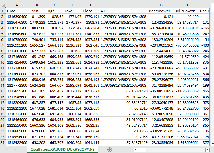
#include <Arrays\ArrayString.mqh>
#include <Arrays\ArrayObj.mqh>
#include <pandas.mqh> //https://www.mql5.com/ja/articles/17030

input datetime start_date = D'2005.01.01';
input datetime end_date = D'2023.01.01';

input string symbol = "XAUUSD";
input ENUM_TIMEFRAMES timeframe = PERIOD_D1;

struct indicator_struct
 {
   long handle;
   CArrayString buffer_names; //buffer_names array
 };

indicator_struct indicators[15]; //Structure for keeping indicator handle alongside its buffer names 
//+------------------------------------------------------------------+
//| Script program start function                                    |
//+------------------------------------------------------------------+
void OnStart()
  {  
//---
   
   vector time, open, high, low, close;
   if (!SymbolSelect(symbol, true))
      {
         printf("%s failed to select symbol %s, Error = %d",__FUNCTION__,symbol,GetLastError());
         return;
      }
   
 //---
   
   time.CopyRates(symbol, timeframe, COPY_RATES_TIME, start_date, end_date);
   open.CopyRates(symbol, timeframe, COPY_RATES_OPEN, start_date, end_date);
   high.CopyRates(symbol, timeframe, COPY_RATES_HIGH, start_date, end_date);
   low.CopyRates(symbol, timeframe, COPY_RATES_LOW, start_date, end_date);
   close.CopyRates(symbol, timeframe, COPY_RATES_CLOSE, start_date, end_date);

   CDataFrame df;
   
   df.insert("Time", time);
   df.insert("Open", open);
   df.insert("High", high);
   df.insert("Low", low);
   df.insert("Close", close);
   
//--- Oscillators
   
   indicators[0].handle = iATR(symbol, timeframe, 14);
   indicators[0].buffer_names.Add("ATR");
   
   indicators[1].handle = iBearsPower(symbol, timeframe, 13);
   indicators[1].buffer_names.Add("BearsPower");
   
   indicators[2].handle = iBullsPower(symbol, timeframe, 13);
   indicators[2].buffer_names.Add("BullsPower");
   
   indicators[3].handle = iChaikin(symbol, timeframe, 3, 10, MODE_EMA, VOLUME_TICK);
   indicators[3].buffer_names.Add("Chainkin");
   
   indicators[4].handle = iCCI(symbol, timeframe, 14, PRICE_OPEN);
   indicators[4].buffer_names.Add("CCI"); 
   
   indicators[5].handle = iDeMarker(symbol, timeframe, 14);
   indicators[5].buffer_names.Add("Demarker");
   
   indicators[6].handle = iForce(symbol, timeframe, 13, MODE_SMA, VOLUME_TICK);
   indicators[6].buffer_names.Add("Force");
   
   indicators[7].handle = iMACD(symbol, timeframe, 12, 26, 9, PRICE_OPEN);
   indicators[7].buffer_names.Add("MACD MAIN_LINE");
   indicators[7].buffer_names.Add("MACD SIGNAL_LINE");
   
   indicators[8].handle = iMomentum(symbol, timeframe, 14, PRICE_OPEN);
   indicators[8].buffer_names.Add("Momentum");
   
   indicators[9].handle = iOsMA(symbol, timeframe, 12, 26, 9, PRICE_OPEN);
   indicators[9].buffer_names.Add("OsMA");
   
   indicators[10].handle = iRSI(symbol, timeframe, 14, PRICE_OPEN);
   indicators[10].buffer_names.Add("RSI");
   
   indicators[11].handle = iRVI(symbol, timeframe, 10);
   indicators[11].buffer_names.Add("RVI MAIN_LINE");
   indicators[11].buffer_names.Add("RVI SIGNAL_LINE");
   
   indicators[12].handle = iStochastic(symbol, timeframe, 5, 3,3,MODE_SMA,STO_LOWHIGH);
   indicators[12].buffer_names.Add("StochasticOscillator MAIN_LINE");
   indicators[12].buffer_names.Add("StochasticOscillator SIGNAL_LINE");
   
   indicators[13].handle = iTriX(symbol, timeframe, 14, PRICE_OPEN);
   indicators[13].buffer_names.Add("TEMA");
   
   indicators[14].handle = iWPR(symbol, timeframe, 14);
   indicators[14].buffer_names.Add("WPR");
   
//--- Get buffers
   
   for (uint ind=0; ind<indicators.Size(); ind++) //Loop through all the indicators
      {
         for (uint buffer_no=0; buffer_no<(uint)indicators[ind].buffer_names.Total(); buffer_no++) //Their buffer names resemble their buffer numbers 
            {
               string name = indicators[ind].buffer_names.At(buffer_no); //Get the name of the buffer, it is helpful for the DataFrame and CSV file
               
               vector buffer = {};
               if (!buffer.CopyIndicatorBuffer(indicators[ind].handle, buffer_no, start_date, end_date)) //Copy indicator buffer 
                  {
                     printf("func=%s line=%d | Failed to copy %s indicator buffer, Error = %d",__FUNCTION__,__LINE__,name,GetLastError());
                     continue;
                  }
               
               df.insert(name, buffer); //Insert a buffer vector and its name to a dataframe object
            }
      }

   df.to_csv(StringFormat("Oscillators.%s.%s.csv",symbol,EnumToString(timeframe)), true); //Save all the data to a CSV file
  }

以下が出力です。

私たちは、MQL5に組み込まれているほぼすべてのオシレーター系インジケーターを収集しました。これらの多くは、最小値と最大値を持つため、定常データを生成します。たとえば、RSIインジケーターは0から100の範囲の値を出力します。

LGMMは、非定常データなど異なる統計的性質を持つデータにも対応可能ですが、定常データは時間を通じて統計的性質が一定に保たれるため、LGMMが意味のある構造やパターンを見つけやすくなります。

もちろん、どのような種類のデータを使用していただいても構いません。

さらに、インジケーターデータに加えて、機械学習用途のためにOpen、High、Low、Close、Time (OHLCT)変数も収集しました。これらの情報は、LGMMだけでなく、可視化や予測型機械学習モデルの目的変数作成にも活用できます。

Pythonスクリプト(Jupyter Notebook)の中では、依存ライブラリをインポートし、MetaTrader 5デスクトップアプリを初期化した直後に、このデータを最初に読み込みます。

ファイル名：main.ipynb

import pandas as pd
import numpy as np
import MetaTrader5 as mt5
import os
from Trade.TerminalInfo import CTerminalInfo
import matplotlib.pyplot as plt
import seaborn
import warnings

warnings.filterwarnings("ignore")
seaborn.set_style("darkgrid")

if not mt5.initialize():
    print("Failed to Initialize MetaTrade5, Error = ",mt5.last_error())
    mt5.shutdown()
    

terminal = CTerminalInfo() # similarly to CTerminalInfo from MQL5. For getting information about the MetaTrader5 app

MQL5を使って保存した共通のパス（フォルダ）からデータをインポートします。

common_path = os.path.join(terminal.common_data_path(), "Files")
symbol = "XAUUSD"
timeframe = "PERIOD_D1"

df = pd.read_csv(os.path.join(common_path, f"Oscillators.{symbol}.{timeframe}.csv")) # the same naming pattern as the one used in the MQL5 script

# Identify max float value
max_float = np.finfo(float).max

# Replace all max float (double) values with NaN produced by preliminary indicator calculations
df = df.replace(max_float, np.nan)
df.dropna(inplace=True)
df["Time"] = pd.to_datetime(df["Time"], unit="s")

df.head()

以下が出力です。

        Time    Open    High    Low     Close   ATR     BearsPower      BullsPower      Chainkin        CCI     ...     MACD SIGNAL_LINE        Momentum        OsMA    RSI     RVI MAIN_LINE   RVI SIGNAL_LINE StochasticOscillator MAIN_LINE  StochasticOscillator SIGNAL_LINE        TEMA    WPR
0       2005-01-03      438.45  438.71  426.72  429.55  5.481429        -12.314215      -0.324215       -1079.046551    -51.013015      ...     0.175727        99.870165       -0.582169       46.666555       -0.082596       0.018515        26.976532       32.920132       -0.000089       -85.144357
1       2005-01-04      429.52  430.18  423.71  427.51  5.450000        -13.677899      -7.207899       -1129.324384    -235.622347     ...     -0.000779       98.615544       -1.252741       37.393138       -0.158362       -0.048541       22.158658       27.150101       -0.000190       -82.774252
2       2005-01-05      427.50  428.77  425.10  426.58  5.162143        -10.743913      -7.073913       -1496.644248    -196.837418     ...     -0.247283       97.044402       -1.816758       35.666584       -0.227422       -0.119850       17.070979       22.068723       -0.000325       -86.990027
3       2005-01-06      426.31  427.85  420.17  421.37  5.234286        -13.606211      -5.926211       -3349.884147    -164.038728     ...     -0.576309       97.480164       -2.194161       34.651526       -0.269634       -0.187300       14.096364       17.775334       -0.000482       -95.312500
4       2005-01-07      421.39  425.48  416.57  419.02  5.605000        -15.098181      -6.188181       -4970.426959    -168.301515     ...     -1.015433       95.440750       -2.669414       30.754440       -0.305796       -0.243045       11.442611       14.203318       -0.000670       -91.609589

後で分類器系の機械学習モデルで利用するために、分類問題用の目的変数を準備します。途中で、インジケーター以外の特徴量は削除されます。

lookahead = 1	

df["future_close"] = df["Close"].shift(-lookahead)
new_df = df.dropna()

new_df["Direction"] = np.where(new_df["future_close"]>new_df["Close"], 1, -1) # if a the close value in the next bar(s)=lookahead is above the current close price, thats a long signal otherwise that's a short signal

from sklearn.model_selection import train_test_split

X = new_df.drop(columns=[
    "Time",
    "Open",
    "High",
    "Low",
    "Close",
    "future_close",
    "Direction"
])

y = new_df["Direction"]

X_train, X_test, y_train, y_test = train_test_split(X, y, test_size=0.2, shuffle=True, random_state=42)

必要なインジケーターデータがあるかどうかを確認する必要があります。

X_train.head()

以下が出力です。

        ATR     BearsPower      BullsPower      Chainkin        CCI     Demarker        MACD MAIN_LINE  MACD SIGNAL_LINE        Momentum        OsMA    RSI     RVI MAIN_LINE   RVI SIGNAL_LINE StochasticOscillator MAIN_LINE  StochasticOscillator SIGNAL_LINE        TEMA    WPR
1057    30.139286       34.958195       62.858195       16280.794393    268.371098      251356.076923   -1.759289       -15.645899      107.768519      13.886610       62.077386       0.229591        0.108028        92.301971       83.886543       -0.002663       -8.048595
3806    3.096429        0.724299        3.314299        -1279.189840    69.806094       696.923077      -0.121217       -0.952863       100.299538      0.831645        52.157089       0.096237        0.080054        67.031250       71.466497       -0.000077       -21.325052
38884   5.927143        -8.488258       -3.858258       -2005.866698    -213.672289     -3333.080000    -0.049837       0.496440        99.774916       -0.546277       39.550361       -0.022395       0.035070        28.046540       49.606252       0.000012        -73.130342
10351   2.060714        -0.491108       1.158892        723.246254      40.384615       2508.735385     1.293179        0.953618        100.533084      0.339561        58.791715       0.217352        0.294053        57.239819       69.770534       0.000123        -19.070322
38170   5.632143        -5.682364       -3.262364       -1321.008995    -109.039933     -1673.607692    -0.609996       0.785433        99.712893       -1.395429       41.917705       -0.062258       -0.053202       13.322009       9.490964        0.000035        -77.826942

最後にLGMMを学習させます。

from sklearn.mixture import GaussianMixture
from skl2onnx import convert_sklearn
from skl2onnx.common.data_types import FloatTensorType

components = 3

gmm = GaussianMixture(n_components=components, covariance_type="full", random_state=42)
gmm.fit(X_train)

latent_features_train = gmm.predict_proba(X_train)
latent_features_test = gmm.predict_proba(X_test)

私はガウス混合モデル(GMM)でコンポーネント数を3つに設定しており、インジケーター上で観測されるパターンを3つのクラスタに分けたいと考えています。1つ目のクラスタは強気トレンド（シグナル）、2つ目のクラスタは弱気トレンド、3つ目のクラスタはレンジ相場を表すと想定しています。 ただし、これはあくまで推測です。

他の教師なし機械学習やクラスタリング手法と同様、モデルが出力するコンポーネント（クラスタ）を直感的に解釈するのは容易ではありません。現時点では、それぞれのコンポーネントが上記の3クラスのどれかに属すると仮定するしかありません。

私がこのモデルを潜在ガウス混合モデル(LGMM)と呼んでいるのに、最終的にはScikit-LearnのGaussianMixtureモデルを使っているのか、不思議に思うかもしれません。

インポートしたGaussianMixtureモデルは、この投稿の数学的背景で説明したLGMMと同等の機能を持っています。理論上、この2つは同じものです。

latent_features_train配列を出力してみましょう。

latent_features_train

以下が出力です。

array([[9.48947877e-13, 1.08107288e-62, 1.00000000e+00],
       [9.71935407e-01, 2.80542130e-02, 1.03801388e-05],
       [5.35722226e-03, 9.94642667e-01, 1.10916653e-07],
       ...,
       [7.72441751e-08, 8.80712550e-41, 9.99999923e-01],
       [9.99975623e-01, 1.07924534e-33, 2.43771745e-05],
       [1.91968188e-01, 8.08030586e-01, 1.22621110e-06]], shape=(3760, 3))

LGMMは、予測結果として各行に3要素の配列を出力しています。各列は、入力されたデータが3つのクラスタのどれに属するかの確率を表しています。すべての行における3列の確率の合計は1になります。。

このままでは解釈が難しいため、モデルをONNX形式に変換し、MQL5上でクラスタを可視化し、この確率的モデルが出力する結果からどのような結論を導けるかを確認してみましょう。

潜在ガウス混合モデル(LGMM)に基づくMQL5インジケーター

まず、LGMMをONNX形式で保存します。

# Define input type (shape should match your training data)
initial_type = [("float_input", FloatTensorType([None, X_train.shape[1]]))]

# Convert the pipeline to ONNX format
onnx_model = convert_sklearn(gmm, initial_types=initial_type)

# Save the model to a file
with open(os.path.join(common_path, f"LGMM.{symbol}.{timeframe}.onnx"), "wb") as f:
    f.write(onnx_model.SerializeToString())

以下は、Netronで開いたときのモデルのアーキテクチャです。

 

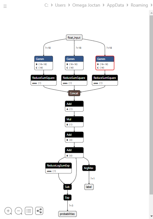
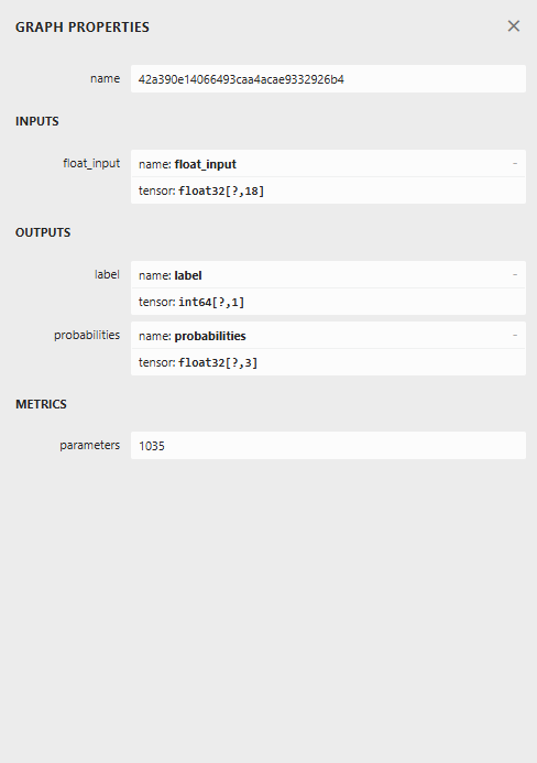
このモデルは少し特殊な構造をしており、最終ノードに2つの出力を持っています。1つは予測ラベル用、もう1つは確率用です。この点を踏まえ、MQL5でこのモデルを読み込むコードを実装する必要があります。

MQL5でLGMMを読み込む 

ファイル名： Gaussian Mixture.mqh

複数の値の配列を受け取る出力構造が必要です。これは、最終ノードに2つの出力があり、それぞれが出力配列を持つためです。

class CGaussianMixture
  {
protected:

   bool initialized;
   long onnx_handle;
   void PrintTypeInfo(const long num,const string layer,const OnnxTypeInfo& type_info);
   
   ulong inputs[]; //Inputs of a model in dimensions [nxn]
   struct outputs_struct 
    {
      ulong outputs[];
    } model_output_structure[];  //Outputs of the model structure array

その後、次が続きます。

bool CGaussianMixture::OnnxLoad(long &handle)
 {
//--- since not all sizes defined in the input tensor we must set them explicitly
//--- first index - batch size, second index - series size, third index - number of series (only Close)
   
   OnnxTypeInfo type_info; //Getting onnx information for Reference In case you forgot what the loaded ONNX is all about

   long input_count=OnnxGetInputCount(handle);
   if (MQLInfoInteger(MQL_DEBUG))
      Print("model has ",input_count," input(s)");
   
   for(long i=0; i<input_count; i++)
     {
      string input_name=OnnxGetInputName(handle,i);
      if (MQLInfoInteger(MQL_DEBUG))
         Print(i," input name is ",input_name);
         
      if(OnnxGetInputTypeInfo(handle,i,type_info))
        {
          if (MQLInfoInteger(MQL_DEBUG))
            PrintTypeInfo(i,"input",type_info);
          ArrayCopy(inputs, type_info.tensor.dimensions);
        }
     }

   long output_count=OnnxGetOutputCount(handle);
   if (MQLInfoInteger(MQL_DEBUG))
      Print("model has ",output_count," output(s)");
   
   ArrayResize(model_output_structure, (int)output_count);
      
   for(long i=0; i<output_count; i++)
     {
      string output_name=OnnxGetOutputName(handle,i);
      if (MQLInfoInteger(MQL_DEBUG))
         Print(i," output name is ",output_name);
         
      if(OnnxGetOutputTypeInfo(handle,i,type_info))
       {
         if (MQLInfoInteger(MQL_DEBUG))
            PrintTypeInfo(i,"output",type_info);
            
         ArrayCopy(model_output_structure[i].outputs, type_info.tensor.dimensions);
       }
       
       //--- Set the output shape
         
         replace(model_output_structure);
         if(!OnnxSetOutputShape(handle, i, model_output_structure[i].outputs))
          {
            if (MQLInfoInteger(MQL_DEBUG))
              {
                printf("Failed to set the Output[%d] shape Err=%d",i,GetLastError());
                DebugBreak();
              }
              
             return false;
          }
     }
   
//---
   
   replace(inputs);
      
//--- Setting the input size

   for (long i=0; i<input_count; i++)   
     if (!OnnxSetInputShape(handle, i, inputs)) //Giving the Onnx handle the input shape
       {
         if (MQLInfoInteger(MQL_DEBUG))
           printf("Failed to set the input shape Err=%d",GetLastError());
         DebugBreak();
         return false;
       }
   
     
   initialized = true;
   if (MQLInfoInteger(MQL_DEBUG))
      Print("ONNX model Initialized");
      
   return true;
 }
//+------------------------------------------------------------------+
//|                                                                  |
//+------------------------------------------------------------------+
bool CGaussianMixture::Init(string onnx_filename, uint flags=ONNX_DEFAULT)
 {  
   onnx_handle = OnnxCreate(onnx_filename, flags);
   
   if (onnx_handle == INVALID_HANDLE)
     return false;
   
   return OnnxLoad(onnx_handle);
 }
//+------------------------------------------------------------------+
//|                                                                  |
//+------------------------------------------------------------------+
bool CGaussianMixture::Init(const uchar &onnx_buff[], ulong flags=ONNX_DEFAULT)
 {  
  onnx_handle = OnnxCreateFromBuffer(onnx_buff, flags); //creating onnx handle buffer 
    
   if (onnx_handle == INVALID_HANDLE)
     return false;
     
  return OnnxLoad(onnx_handle);
 }

私たちは、このクラスの予測メソッドを修正し、予測ラベルと確率ベクトルの2つの変数を構造体で返す仕様にしました。

struct pred_struct
 {
   vector proba;
   long label;
 };

pred_struct CGaussianMixture::predict(const vector &x)
 {
   pred_struct res;
   
   if (!this.initialized)
    {
      if (MQLInfoInteger(MQL_DEBUG))
         printf("%s The model is not initialized yet to make predictions | call Init function first",__FUNCTION__);
         
      return res;
    }
   
//---
   
   vectorf x_float; //Convert inputs from a vector of double values to those float values
   x_float.Assign(x);
   
   vector label = vector::Zeros(model_output_structure[0].outputs[1]); //outputs[1] we get the second shape (columns) from an array
   vector proba = vector::Zeros(model_output_structure[1].outputs[1]); //outputs[1] we get the second shape (columns) from an array
    
   if (!OnnxRun(onnx_handle, ONNX_DATA_TYPE_FLOAT, x_float, label, proba)) //Run the model and get the predicted label and probability
     {
       if (MQLInfoInteger(MQL_DEBUG))
          printf("Failed to get predictions from Onnx err %d",GetLastError());
       
       DebugBreak();   
       return res;
     }
     
//---

   res.label = (long)label[label.Size()-1]; //Get the last item available at the label's array
   res.proba = proba;
   
   return res;
 }

インジケーターのmain関数内で予測関数を呼び出し、潜在特徴量を取得するようにします。

ファイル名： LGMM Indicator.mq5

int OnCalculate(const int32_t rates_total,
                const int32_t prev_calculated,
                const datetime &time[],
                const double &open[],
                const double &high[],
                const double &low[],
                const double &close[],
                const long &tick_volume[],
                const long &volume[],
                const int32_t &spread[])
  {      
//--- Main calculation loop
   
   int lookback = 20;
   
   for (int i = prev_calculated; i < rates_total && !IsStopped(); i++)
   {      
      if (i+1<lookback) //prevent data not found errors during copy buffer
         continue;
         
      int reverse_index = rates_total - 1 - i;
      
      //--- Get the indicators data
      
      vector x = getX(reverse_index, lookback);
      
      if (x.Size()==0)
         continue;
         
      pred_struct res = lgmm.predict(x);
      
      vector proba = res.proba;
      long label = res.label;
      
      ProbabilityBuffer[i] = proba.Max();
      
      // Determine color based on histogram value
      
      if (label == 0)
         ColorBuffer[i] = 0;
      else if (label == 1)
         ColorBuffer[i] = 1; 
      else
         ColorBuffer[i] = 2; 
     
      Comment("bars [",i+1,"/",rates_total,"]"," Proba: ",proba," label: ",label);
   }
   
//--- 
   return(rates_total);
  }

getX()関数の中では、学習用データを収集したスクリプトと同じ方法で、すべてのインジケーターバッファを収集する必要があります。

vector getX(uint start=0, uint count=10)
 {
//--- Get buffers

   CDataFrame df;
   for (uint ind=0; ind<indicators.Size(); ind++) //Loop through all the indicators
      {    
        uint buffers_total = indicators[ind].buffer_names.Total();
        
         for (uint buffer_no=0; buffer_no<buffers_total; buffer_no++) //Their buffer names resemble their buffer numbers 
            {
               string name = indicators[ind].buffer_names.At(buffer_no); //Get the name of the buffer, it is helpful for the DataFrame and CSV file
               
               vector buffer = {};
               if (!buffer.CopyIndicatorBuffer(indicators[ind].handle, buffer_no, start, count)) //Copy indicator buffer 
                  {
                     printf("func=%s line=%d | Failed to copy %s indicator buffer, Error = %d",__FUNCTION__,__LINE__,name,GetLastError());
                     continue;
                  }
               
               df.insert(name, buffer); //Insert a buffer vector and its name to a dataframe object
            }
      }
         
   return df.iloc(-1); //Return the latest information from the dataframe which is the most recent buffer
 }

補足：すべてのインジケーターは、モデルを共通フォルダから初期化した直後のInit関数内で初期化されています。この共通フォルダは、Pythonで保存した場所です。 

#include <Gaussian Mixture.mqh>
#include <Arrays\ArrayString.mqh>
#include <MALE5\Pandas\pandas.mqh>

CGaussianMixture lgmm;

input string symbol = "XAUUSD";
input ENUM_TIMEFRAMES timeframe = PERIOD_D1;

struct indicator_struct
 {
   long handle;
   CArrayString buffer_names;
 };

indicator_struct indicators[15];

//--- Indicator buffers

double ProbabilityBuffer[];
double ColorBuffer[];
double MaBuffer[];
//+------------------------------------------------------------------+
//| Custom indicator initialization function                         |
//+------------------------------------------------------------------+
int OnInit()
  {
//--- indicator buffers mapping
   
   Comment("");
   
   // Setting indicator properties
   SetIndexBuffer(0, ProbabilityBuffer, INDICATOR_DATA);
   SetIndexBuffer(1, ColorBuffer, INDICATOR_COLOR_INDEX);
   
   // Setting histogram drawing style
   PlotIndexSetInteger(0, PLOT_DRAW_TYPE, DRAW_COLOR_HISTOGRAM);
   
   // Set indicator labels
   IndicatorSetString(INDICATOR_SHORTNAME, "3-Color Histogram");
   IndicatorSetInteger(INDICATOR_DIGITS, _Digits);
   
//---
   
   string filename = StringFormat("LGMM.%s.%s.onnx",symbol, EnumToString(timeframe));
   if (!lgmm.Init(filename, ONNX_COMMON_FOLDER))
      {
         printf("%s Failed to initialize the GaussianMixture model (LGMM) in ONNX format file={%s}, Error = %d",__FUNCTION__,filename,GetLastError());
      }
   
//--- Oscillators
   
   indicators[0].handle = iATR(symbol, timeframe, 14);
   indicators[0].buffer_names.Add("ATR");
   
   //...
   //...
   //...
   
   indicators[14].handle = iWPR(symbol, timeframe, 14);
   indicators[14].buffer_names.Add("WPR");
   
   for (uint i=0; i<indicators.Size(); i++)   
     if (indicators[i].handle==INVALID_HANDLE)
        {
          printf("%s Invalid %s handle, Error = %d",__FUNCTION__,indicators[i].buffer_names[0],GetLastError());
          return INIT_FAILED;
        }
           
//---
   return(INIT_SUCCEEDED);
  }

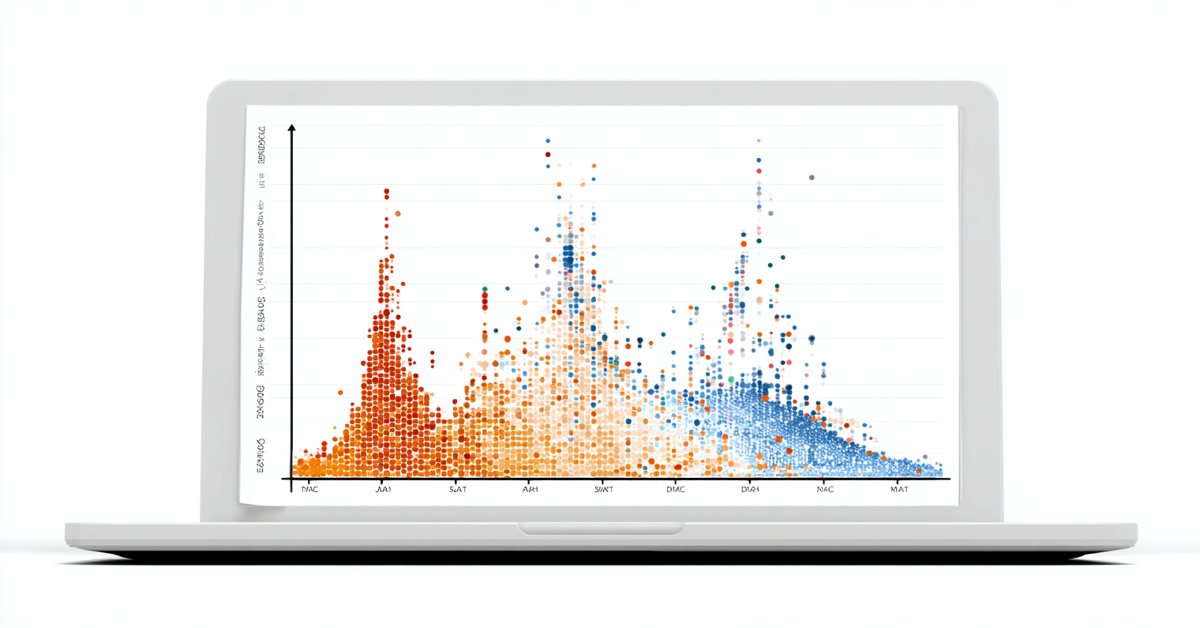
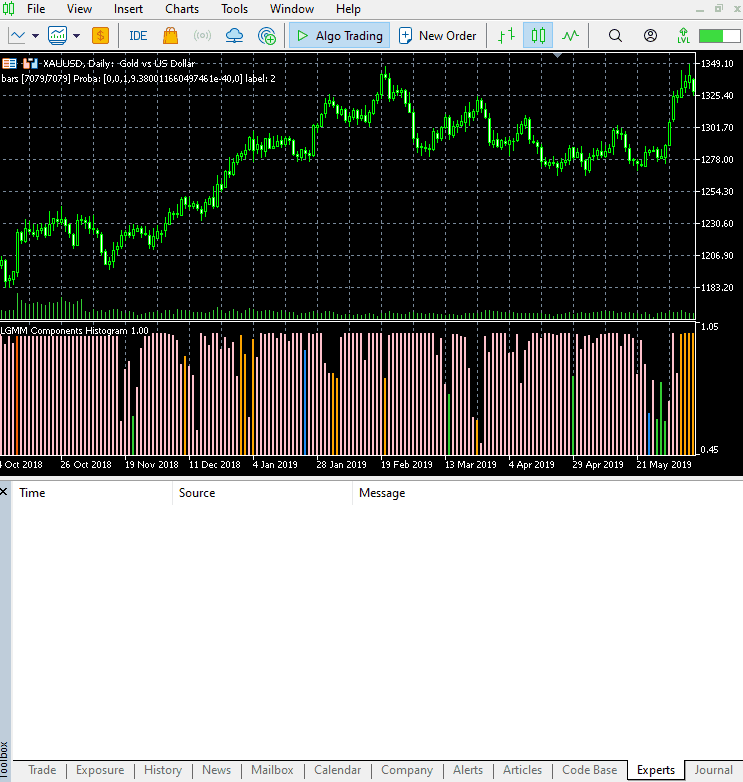
最後に、このインジケーターをXAUUSDのチャート上で、モデルを学習したのと同じ時間足で実行します。

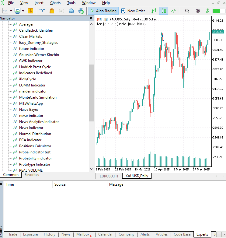
このインジケーターもまだ解釈は容易ではありませんが、赤色で表示されているコンポーネントが支配的なパターンとして目立ちます。このパターンは、相場が上昇トレンドと下降トレンドのいずれであっても、ボラティリティが高いときに現れるようです。残りのコンポーネントについてはまだはっきりしていません。これは、モデルで使用したコンポーネント数が最適かどうか確信が持てないことが原因かもしれません。そこで、このモデルに対して最適なコンポーネント数を見つけてみましょう。

LGMMにおける最適なコンポーネント数の探索

Scikit-Learnが提供する混合モデルは、情報量規準の値、つまり赤池情報量規準(AIC)とベイズ情報量規準(BIC)を出力することができます。これらの値をコンポーネント数の範囲に対してプロットし、肘のように見える点を探してみましょう。

グラフにおいて肘のように見える点とは、モデルにコンポーネントを追加しても性能の向上がわずかになり、曲線が平坦になるポイントのことです。

ファイル名：main.ipynb

lowest_bic = np.inf
bic = []
aic = []
n_components_range = range(1, 10)

for n_components in n_components_range:
    gmm = GaussianMixture(n_components=n_components, random_state=42)
    gmm.fit(X)
    bic.append(gmm.bic(X_train))
    aic.append(gmm.aic(X_train))
    if bic[-1] < lowest_bic:
        best_gmm = gmm
        lowest_bic = bic[-1]

# Plot the BIC and AIC scores
plt.figure(figsize=(8, 5))
plt.plot(n_components_range, bic, label='BIC', marker='o')
plt.plot(n_components_range, aic, label='AIC', marker='o')
plt.xlabel('Number of components')
plt.ylabel('Score')
plt.title('LGMM selection: AIC vs BIC')
plt.legend()
plt.grid(True)
plt.show()

以下が出力です。

AIC曲線とBIC曲線の両方は、コンポーネント数が1から2に増えると急激に下がり、その後も減少を続けますが、コンポーネント数が5を超えると改善の度合いが明らかに緩やかになります。これは、このモデルで使用すべき最適なコンポーネント数が5であることを示しています。

それでは、モデルを再学習させて、インジケーターを更新しましょう。

ファイル名：main.ipynb

components = 5 # according to the elbow point

gmm = GaussianMixture(n_components=components, covariance_type="full", random_state=42)
gmm.fit(X_train)

latent_features_train = gmm.predict_proba(X_train)
latent_features_test = gmm.predict_proba(X_test)

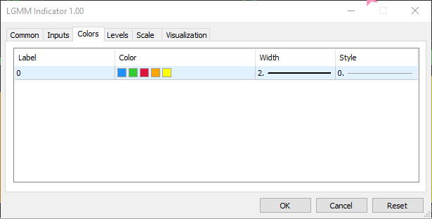
これで、3次元空間に5つのコンポーネントが入り、プロットできる確率が5つになったため、インジケーターのカラーヒストグラム用の色数を5色に増やし、予測ラベルの5つの異なるケースを処理する必要があります。

ファイル名：LGMM Indicator.mq5

#property indicator_color1  clrDodgerBlue, clrLimeGreen, clrCrimson, clrOrange, clrYellow

以下は、OnCalculate関数の内部です。

int OnCalculate(const int32_t rates_total,
                const int32_t prev_calculated,
                const datetime &time[],
                const double &open[],
                const double &high[],
                const double &low[],
                const double &close[],
                const long &tick_volume[],
                const long &volume[],
                const int32_t &spread[])
  {      
//--- Main calculation loop
   
   int lookback = 20;
   
   for (int i = prev_calculated; i < rates_total && !IsStopped(); i++)
   {      
      if (i+1<lookback) //prevent data not found errors during copy buffer
         continue;
         
      //...
      //...
      //...
      
      // Determine color based on predicted label
      
      if (label == 0)
         ColorBuffer[i] = 0;
      else if (label == 1)
         ColorBuffer[i] = 1; 
      else if (label == 2)
         ColorBuffer[i] = 2; 
      else if (label == 3)
         ColorBuffer[i] = 3; 
      else
         ColorBuffer[i] = 4; 
     
      Comment("bars [",i+1,"/",rates_total,"]"," Proba: ",proba," label: ",label);
   }

以下は、新しいインジケーターの外観です。

見た目は良くなりましたが、やはり読み取りは難しいです。私たちは普段、売られ過ぎや買われ過ぎの領域を示す単純なオシレーターに慣れているためです。このインジケーターを自由に試してみて、ディスカッション欄で感想を共有してください。

次はLGMMを機械学習モデルと組み合わせて使ってみましょう。

潜在ガウス混合モデルと分類器モデルの併用

これまでに、LGMMを使って各ラベルが特定のクラスタに属する確率を表す潜在特徴量を生成する方法を確認しました。しかし、これらの特徴量は解釈が難しいため、次はこれをランダムフォレスト分類器に組み込み、インジケーターの特徴量とともに使ってみましょう。この機械学習モデルが、潜在特徴量が取引シグナルにどのように影響するかを学習してくれることを期待します。

ファイル名：main.ipynb

なお、目的変数（予測ラベル）は、以前に学習用用とテスト用データを分割した際にすでに作成しています。ここでも参考のため再掲します。

from sklearn.model_selection import train_test_split

X = new_df.drop(columns=[
    "Time",
    "Open",
    "High",
    "Low",
    "Close",
    "future_close",
    "Direction"
])

y = new_df["Direction"]

X_train, X_test, y_train, y_test = train_test_split(X, y, test_size=0.2, shuffle=True, random_state=42)

LGMMを学習させた後、学習データとテストデータに対して予測をおこないました。

latent_features_train = gmm.predict_proba(X_train)
latent_features_test = gmm.predict_proba(X_test)

このデータは読み取りが難しいため、特徴量に名前を付けて識別可能にしましょう。

latent_features_train_df = pd.DataFrame(latent_features_train, columns=[f"LATENT_FEATURE_{i}" for i in range(latent_features_train.shape[1])])
latent_features_test_df = pd.DataFrame(latent_features_test, columns=[f"LATENT_FEATURE_{i}" for i in range(latent_features_test.shape[1])])

latent_features_train_df

以下が出力です。

	LATENT_FEATURE_0	LATENT_FEATURE_1	LATENT_FEATURE_2	LATENT_FEATURE_3	LATENT_FEATURE_4
0	0.000000e+00	5.368039e-08	9.999999e-01	1.566000e-57	8.541983e-37
1	3.316692e-124	8.262106e-01	2.931424e-06	1.725415e-01	1.244990e-03
2	6.572730e-49	7.441120e-08	3.481699e-08	9.461818e-01	5.381811e-02
3	0.000000e+00	1.165057e-126	1.413762e-05	4.101964e-16	9.999859e-01
4	0.000000e+00	4.446778e-289	1.000000e+00	1.717945e-36	4.234123e-21

これらの特徴量を主要な指標データと並べてみます。

all_columns = X_train.columns.tolist() + latent_features_train_df.columns.tolist()

X_latent_train_arr = np.hstack([X_train, latent_features_train_df])
X_latent_test_arr = np.hstack([X_test, latent_features_test_df])

X_Train_latent = pd.DataFrame(X_latent_train_arr, columns=all_columns)
X_Test_latent = pd.DataFrame(X_latent_test_arr, columns=all_columns)

X_Train_latent.columns

以下が出力です。

Index(['ATR', 'BearsPower', 'BullsPower', 'Chainkin', 'CCI', 'Demarker',
       'Force', 'MACD MAIN_LINE', 'MACD SIGNAL_LINE', 'Momentum', 'OsMA',
       'RSI', 'RVI MAIN_LINE', 'RVI SIGNAL_LINE',
       'StochasticOscillator MAIN_LINE', 'StochasticOscillator SIGNAL_LINE',
       'TEMA', 'WPR', 'LATENT_FEATURE_0', 'LATENT_FEATURE_1',
       'LATENT_FEATURE_2', 'LATENT_FEATURE_3', 'LATENT_FEATURE_4'],
      dtype='object')

この結合されたデータをランダムフォレスト分類器に渡してみましょう。

from sklearn.ensemble import RandomForestClassifier
from sklearn.utils.class_weight import compute_class_weight

classes = np.unique(y_train)
weights = compute_class_weight(class_weight='balanced', classes=classes, y=y_train)

class_weights_dict = dict(zip(classes, weights))

params = {
    "n_estimators": 100,
    "min_samples_split": 2,
    "max_depth": 10,
    "max_leaf_nodes": 10,
    "criterion": "gini",
    "random_state": 42
}

model = RandomForestClassifier(**params, class_weight=class_weights_dict)

model.fit(X_Train_latent, y_train)

以下がモデルの評価です。

y_train_pred = model.predict(X_Train_latent)

print("Train classification report\n", classification_report(y_train, y_train_pred))

y_test_pred = model.predict(X_Test_latent)

print("Test classification report\n", classification_report(y_test, y_test_pred))

以下が出力です。

Train classification report
               precision    recall  f1-score   support

          -1       0.60      0.67      0.63      1766
           1       0.68      0.61      0.64      1994

    accuracy                           0.64      3760
   macro avg       0.64      0.64      0.64      3760
weighted avg       0.64      0.64      0.64      3760

Test classification report
               precision    recall  f1-score   support

          -1       0.45      0.47      0.45       445
           1       0.50      0.48      0.49       495

    accuracy                           0.47       940
   macro avg       0.47      0.47      0.47       940
weighted avg       0.47      0.47      0.47       940

作成したモデルは、検証サンプルに対する性能があまり良くありません。改善できる点は多くありますが、ひとまずモデルが出力する特徴量の重要度プロットを観察してみましょう。

importances = model.feature_importances_
feature_names = X_Train_latent.columns if hasattr(X_Train_latent, 'columns') else [f'feature_{i}' for i in range(X_Train_latent.shape[1])]

# Create DataFrame and sort
importance_df = pd.DataFrame({'feature': all_columns, 'importance': importances})
importance_df = importance_df.sort_values('importance', ascending=False)

# Plot
plt.figure(figsize=(8, 6))
plt.barh(importance_df['feature'], importance_df['importance'], color='red')
plt.title('RFC Feature Importance (Gini Importance)')
plt.xlabel('Importance Score')
plt.gca().invert_yaxis()  # Most important on top
plt.show()

以下が出力です。

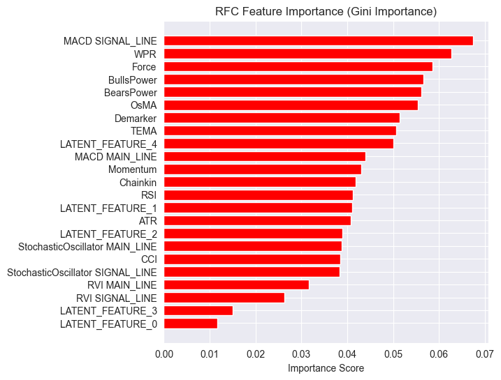
潜在特徴量はモデルにとって重要であることがわかります。つまり、これらはモデルの予測に寄与するパターンや情報を持っているということです。

このモデルの性能が低い理由の一つは、使用している目的変数の性質にあるかもしれません。現在のlookahead値が1では正しくない可能性があります。

通常、これらのインジケーターを使って取引判断を行う場合、次の1本のバーだけを予測するわけではありません。たとえば、RSI値が閾値30以下（売られ過ぎ）の場合、数本先のバーで市場が強気に転じる可能性があると判断します。しかし、現在のモデルでは次のバーだけを予測するように学習させています。

そこで、目的変数をlookahead値5を使って再作成しましょう。

lookahead = 5

df["future_close"] = df["Close"].shift(-lookahead)
new_df = df.dropna()

new_df["Direction"] = np.where(new_df["future_close"]>new_df["Close"], 1, -1) # if a the close value in the next bar(s)=lookahead is above the current close price, thats a long signal otherwise that's a short signal

学習データと検証データの両方でモデルを評価すると、異なる結果が生成されます。

Train classification report
               precision    recall  f1-score   support

          -1       0.56      0.70      0.62      1706
           1       0.69      0.54      0.61      2050

    accuracy                           0.61      3756
   macro avg       0.62      0.62      0.61      3756
weighted avg       0.63      0.61      0.61      3756

Test classification report
               precision    recall  f1-score   support

          -1       0.46      0.61      0.52       392
           1       0.63      0.48      0.55       548

    accuracy                           0.54       940
   macro avg       0.55      0.55      0.53       940
weighted avg       0.56      0.54      0.54       940

特徴量重要度プロットも異なります。

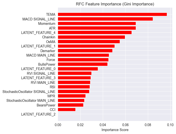
モデルの全体的な精度は54%で、決して高くはありませんが、特徴量重要度プロットで見ている内容を信じるには十分なレベルです。

LGMMが生成した潜在特徴量のいくつかは、モデルにおける最も予測力の高い特徴量の上位にランクイン しています。

たとえば、LATENT_FEATURE_4はランダムフォレスト分類器における5番目に重要な特徴量であり、LATENT_FEATURE_0やLATENT_FEATURE_1などの他の潜在特徴量もかなり良い結果を出しており、一部の生のインジケーターよりも優れていることが分かります。

全体的に見て、LGMMが生成したほとんどの特徴量は、分類器モデルにとって有益なパターンを含んでいることがわかります。

この情報を踏まえ、これでインジケーターを理解するための出発点が得られたことになります。

色の配置は潜在特徴量に似ています。

LGMMを用いた自動売買ロボット

エキスパートアドバイザー(EA)内では、まず必要なライブラリをインポートすることから始めます。

ファイル名： LGMM BASED EA.mq5

#include <Random Forest.mqh>
#include <Arrays\ArrayString.mqh>
#include <pandas.mqh> //https://www.mql5.com/ja/articles/17030
#include <Trade\Trade.mqh>
#include <Trade\PositionInfo.mqh>
#include <Trade\SymbolInfo.mqh>
#include <errordescription.mqh>

CSymbolInfo m_symbol;
CTrade m_trade;
CPositionInfo m_position;
CRandomForestClassifier rfc;

繰り返しになりますが、学習データで使用されているものと同じ銘柄と時間足を使用していることを確認する必要があります。

#define MAGICNUMBER 11062025

input string SYMBOL = "XAUUSD";
input ENUM_TIMEFRAMES TIMEFRAME = PERIOD_D1;
input uint LOOKAHEAD = 5;
input uint SLIPPAGE = 100;

OnInit関数内で、LGMMとランダムフォレスト分類モデルの両方のモデルを初期化します。

int OnInit()
  {

   if (!MQLInfoInteger(MQL_DEBUG) && !MQLInfoInteger(MQL_TESTER))
    {
      ChartSetSymbolPeriod(0, SYMBOL, TIMEFRAME);
      if (!SymbolSelect(SYMBOL, true))
         {
            printf("%s failed to select SYMBOL %s, Error = %s",__FUNCTION__,SYMBOL,ErrorDescription(GetLastError()));
            return INIT_FAILED;
         }
    }

//--- Loading the Gaussian Mixture model

   string filename = StringFormat("LGMM.%s.%s.onnx",SYMBOL, EnumToString(TIMEFRAME));
   if (!lgmm.Init(filename, ONNX_COMMON_FOLDER))
      {
         printf("%s Failed to initialize the GaussianMixture model (LGMM) in ONNX format file={%s}, Error = %s",__FUNCTION__,filename,ErrorDescription(GetLastError()));
      }
   
//--- Loading the RFC model
   
   filename = StringFormat("rfc.%s.%s.onnx",SYMBOL,EnumToString(TIMEFRAME));
   Print(filename);
   if (!rfc.Init(filename, ONNX_COMMON_FOLDER))
      {
         printf("func=%s line=%d, Failed to Load the RFC in ONNX file={%s}, Error = %s",__FUNCTION__,__LINE__,filename,ErrorDescription(GetLastError()));
         return INIT_FAILED;
      }
//...
//... other lines of code
//...
}

getX関数内では、LGMMを呼び出して、ランダムフォレスト分類モデルの最終入力の指標データと一緒に使用できる潜在な特徴量を準備します。

vector getX(uint start=0, uint count=10)
 {
//--- Get buffers

   CDataFrame df;
   for (uint ind=0; ind<indicators.Size(); ind++) //Loop through all the indicators
      {    
        uint buffers_total = indicators[ind].buffer_names.Total();
        
         for (uint buffer_no=0; buffer_no<buffers_total; buffer_no++) //Their buffer names resemble their buffer numbers 
            {
               string name = indicators[ind].buffer_names.At(buffer_no); //Get the name of the buffer, it is helpful for the DataFrame and CSV file
               
               vector buffer = {};
               if (!buffer.CopyIndicatorBuffer(indicators[ind].handle, buffer_no, start, count)) //Copy indicator buffer 
                  {
                     printf("func=%s line=%d | Failed to copy %s indicator buffer, Error = %d",__FUNCTION__,__LINE__,name,GetLastError());
                     continue;
                  }
               
               df.insert(name, buffer); //Insert a buffer vector and its name to a dataframe object
            }
      }
   
   if ((uint)df.shape()[0]==0)
      return vector::Zeros(0);
   
//--- predict the latent features

   vector indicators_data = df.iloc(-1); //index=-1 returns the last row from the dataframe which is the most recent buffer from all indicators
   
//--- Given the indicators let's predict the latent features
   
   vector latent_features = lgmm.predict(indicators_data).proba;
   
   if (latent_features.Size()==0)
      return vector::Zeros(0);
         
   return hstack(indicators_data, latent_features); //Return indicators data stacked alongside latent features 
 }

最後に、ランダムフォレスト分類モデルによって生成された取引シグナルに依存するシンプルな取引戦略を作成します。

void OnTick()
  {
//--- Close trades after AI predictive horizon is over

   CloseTradeAfterTime(MAGICNUMBER, PeriodSeconds(TIMEFRAME)*LOOKAHEAD);
   
//--- Refresh tick information

   if (!m_symbol.RefreshRates())
     {
       printf("func=%s line=%s. Failed to copy rates, Error = %s",__FUNCTION__,ErrorDescription(GetLastError()));
       return;
     }
      
//---

    vector x = getX(); //Get all the input for the model
    
    if (x.Size()==0)
      return;
    
    long signal = rfc.predict(x).cls; //the class predicted by the random forest classifier
    double proba = rfc.predict(x).proba; //probability of the predictions
    
    double volume = m_symbol.LotsMin();
      
    if (!PosExists(POSITION_TYPE_SELL, MAGICNUMBER) && !PosExists(POSITION_TYPE_BUY, MAGICNUMBER)) //no position is open
      {
        if (signal == 1) //If a model predicts a bullish signal
          m_trade.Buy(volume, SYMBOL, m_symbol.Ask()); //Open a buy trade 
        else if (signal == -1) // if a model predicts a bearish signal
          m_trade.Sell(volume, SYMBOL, m_symbol.Bid()); //open a sell trade
      }
  }

モデルが学習した時間足でLOOKAHEAD数のバーが経過したら、取引を終了します。LOOKAHEAD値は、学習スクリプト内で目的変数を作成するときに使用される値と一致する必要があります。

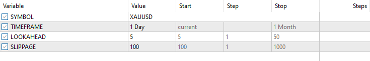
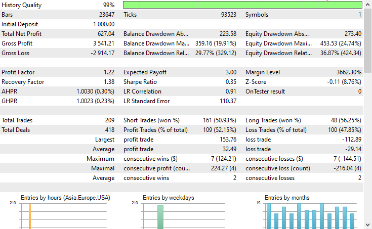
以下はテスターの構成です。

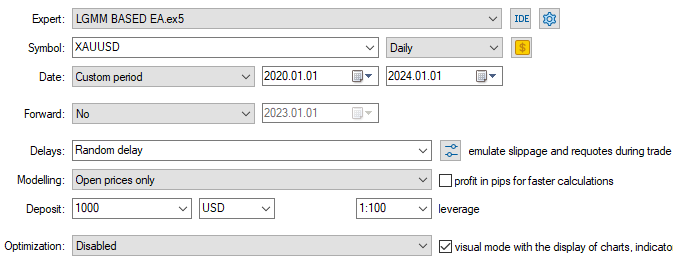
以下が入力です。

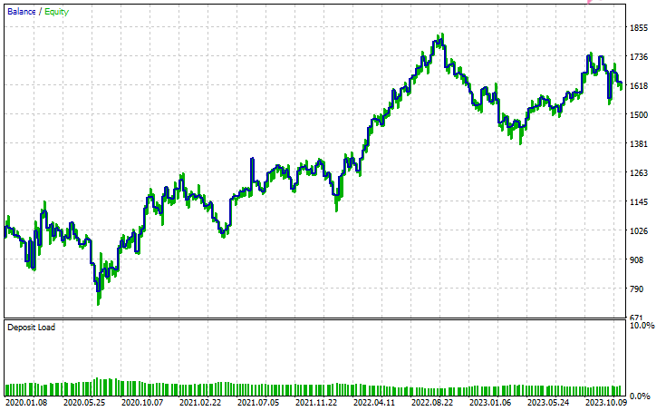
以下がテスターの結果です。

結論

潜在ガウス混合モデル(LGMM)は、非観測パターンを含む意味のある特徴量を抽出できる優れた手法であり、機械学習モデルにとって有用な情報を提供してくれます。しかし、他の機械学習モデルや予測手法と同様に、いくつかの欠点も存在します。

潜在ガウス混合モデル(LGMM)：概要

側面	説明
LGMMとは	データ中の非観測パターンを表す潜在（隠れた）特徴量を抽出する手法です。これらの特徴量は機械学習モデルで有用に活用できます。
主な利点	データ中の意味のある隠れた構造を捉えることができ、モデルの性能向上に寄与します。

LGMMの制約

制限	説明
正規分布を前提	LGMMは各データ点が多変量正規分布に従うと仮定します。しかし、金融データは混沌として非線形であることが多く、この前提は必ずしも成立しません。
初期値に敏感	コンポーネント数の選択や初期化が重要です。不適切な初期化やパラメータ設定は、モデルの有効性を大きく低下させる可能性があります。
結果の解釈が難しい	LGMMが生成する潜在特徴量は理解や説明が難しいです。教師なし手法であるため、検出したパターンにラベルを付けず、単にクラスタリングするだけです。
外れ値に敏感	正規分布は外れ値に対して頑健ではありません。極端な値がいくつかあるだけで平均が歪み、分散が膨らみ、モデルの結果を歪めることがあります。

このモデルは、次元削減（特徴量を少数の意味のある特徴量にまとめる）や新しい特徴量を導入してモデルを豊かにする目的で使用するのが最も有用です。私は、このような使い方が最適だと考えています。

ご一読、誠にありがとうございました。

今後の更新にもご注目ください。こちらのGitHubリポジトリで、MQL5言語向けの機械学習アルゴリズムの開発にぜひ貢献してください。

添付ファイルの表

ファイル名	説明と使用法
Include\errordescription.mqh	MetaTrader 5 が生成するすべてのエラーコードの説明を含むファイル（MQL5言語用）
Include\Gaussian Mixture.mqh	ONNX形式で保存されたガウス混合モデルを初期化して展開するためのクラスを含むライブラリ
Include\pandas.mqh	PythonのPandasに似た、データの格納と操作を行うクラスを含むファイル
Include\Random Forest.mqh	ONNX形式で保存されたランダムフォレスト分類器を初期化して展開するためのクラスを含むライブラリ
Indicators\LGMM Indicator.mq5	潜在ガウス混合モデル(LGMM)が生成した潜在特徴量を表示するためのインジケーター
Scripts\Get XAUUSD Data.mq5	MetaTrader 5からオシレーター指標とOHLCT値を収集し、CSVファイルに保存するスクリプト
Experts\LGMM BASED EA.mq5	LGMMで生成した潜在特徴量とオシレーター指標を組み合わせたデータを使用して、ランダムフォレスト分類器の予測に基づき売買をおこなうEA
Python Code\main.ipynb	データ分析や機械学習モデルの学習などをおこなうためのJupyter Notebook（Pythonスクリプト）
Python Code\Trade\TerminalInfo.py	MQL5のCTerminalInfoに似たクラスを提供し、選択されたMetaTrader 5デスクトップアプリの情報を取得するためのファイル
Python\requirements.txt	本プロジェクトで使用されたPython依存ライブラリとそのバージョンを記載したファイル
Common\Files\*	サンプルCSV（学習データ）および本記事で使用したONNXモデルファイルの一部を格納。参照用。