

数据科学与机器学习(第四十四部分):利用向量自回归(VAR)预测外汇 OHLC 时间序列
 206
206
 0
0

内容
- 什么是向量自回归(VAR)
- 向量自回归(VAR)模型的数学原理
- VAR 模型的基本假设
- 在 Python 中对 OHLC 值实现 VAR 模型
- 使用 VAR 进行样本外预测
- 构建基于 VAR 的交易机器人
- 最后的思考
什么是向量自回归(VAR)?
这是一种传统的统计时间序列预测工具,用于研究多个时间序列变量之间的动态关系。与单变量自回归模型(如 ARIMA,在上一篇文章中讨论过)仅基于自身历史值预测单个变量不同,VAR 模型研究多个变量之间的相互关联性。
它们通过将每个变量建模为不仅是其自身历史值的函数,也是系统中其他变量历史值的函数来实现这一点。在本文中,我们将探讨向量自回归的基本原理及其在交易中的应用。
模型起源
向量自回归由经济学家克莱夫・格兰杰(Clive Granger)于 20 世纪 60 年代首次提出。格兰杰的重大发现为理解和建模经济因素之间存在的动态相互作用奠定了框架。在 20 世纪 70 年代和 80 年代,VAR 模型在计量经济学和宏观经济学领域获得了显著发展。
该技术是自回归(AR)模型的多变量扩展。传统的 AR 模型(如 ARIMA)分析单个变量与其滞后值之间的关系,而 VAR 模型同时考虑多个变量。在 VAR 模型中,每个变量都对其自身的滞后值以及系统中其他变量的滞后值进行回归。
在本系列的上一篇文章中,我们讨论了 ARIMA,并发现它无法将多个变量纳入其训练和预测过程。在本文中,我们将讨论 VAR,很多人可能会认为它是 ARIMA 的前身,因为它旨在解决单变量时间序列预测的问题。
为了理解这个简单的技术(模型),让我们来看看它的数学原理。
向量自回归(VAR)模型的数学原理
其他自回归模型(AR、ARMA 和 ARIMA)与 VAR 模型的主要区别在于,前者是单向的(预测变量影响目标变量,反之则不然),而 VAR 是双向的。
数学上,一个具有 'p' 阶滞后的 VAR (p) 模型可以表示为:

其中:
- c = 模型的常数项(截距)
-
 = 直到 p 阶的 Y 滞后项的系数
 -
 = 时间 t 处的时间序列值
 -
 = 时间 t 处的误差项
一个 k 维、p 阶的 VAR 模型,记为 VAR (p),考虑 k=2 时,方程如下:

对于 VAR 模型,我们有多个相互影响的时间序列变量;它被建模为一个方程组,每个时间序列变量对应一个方程。以下是矩阵形式的公式:

最终的 VAR 方程为:

为确保从 VAR 模型获得的结果的有效性和可信度,必须满足各种假设和要求。
VAR 模型的基本假设
- 线性
正如我们从其公式中看到的,VAR 本质上是一个线性模型,因此该模型中使用的所有变量都必须是线性的(即表示为滞后值的加权和)。 - 平稳性
该模型中使用的所有变量都必须是平稳的,即时间序列每个特征的均值、方差和协方差必须随时间保持不变。如果数据集中存在非平稳特征,我们必须将其全部转换为平稳特征。 - 特征之间不存在完全多重共线性
为使 VAR 有效工作,任何解释变量都不能是其他变量的精确线性组合。这一点很重要,因为它有助于防止 OLS 估计中出现奇异矩阵(即矩阵 必须可逆)。我们必须删除冗余特征或使用正则化技术来解决这个问题
。 - 残差无自相关
该模型假设残差不存在序列相关,应为白噪声。自相关会使标准误产生偏差,并使统计检验失效。 - 充足的观测值
VAR 假设已获得足够的数据用于参数估计。因此,我们需要为模型提供尽可能多的信息,以实现最大效率。
现在让我们看看如何用 Python 编程语言实现这个模型。
在 Python 中对 OHLC 值实现 VAR 模型
首先安装所有 Python 依赖项,requirements.txt 文件可在附件部分找到。
pip install -r requirements.txt
导入库。
import pandas as pd
import numpy as np
import seaborn as sns
import matplotlib.pyplot as plt
import warnings

# Suppress all warnings
warnings.filterwarnings("ignore")

sns.set_style("darkgrid")
我们首先从 MetaTrader 5 中导入开盘价、最高价、最低价和收盘价(OHLC)数据。
symbol = "EURUSD"
timeframe = mt5.TIMEFRAME_D1

if not mt5.symbol_select(symbol, True):
    print("Failed to select and add a symbol to the MarketWatch, Error = ",mt5.last_error)
    quit()

rates = mt5.copy_rates_from_pos(symbol, timeframe, 1, 10000)
df = pd.DataFrame(rates) # convert rates into a pandas dataframe

df
输出。
| 时间 | 开盘价 | 最高价 | 最低价 | 收盘价 | tick成交量 | 点差 | 真实成交量 | |
|---|---|---|---|---|---|---|---|---|
| 0 | 611280000 | 1.00780 | 1.01050 | 1.00630 | 1.00760 | 821 | 50 | 0 |
| 1 | 611366400 | 0.99620 | 1.00580 | 0.99100 | 0.99600 | 2941 | 50 | 0 |
| 2 | 611452800 | 0.99180 | 0.99440 | 0.98760 | 0.99190 | 1351 | 50 | 0 |
| 3 | 611539200 | 0.99330 | 0.99370 | 0.99310 | 0.99310 | 101 | 50 | 0 |
| 4 | 611798400 | 0.97360 | 0.97360 | 0.97320 | 0.97360 | 81 | 50 | 0 |
| ... | ... | ... | ... | ... | ... | ... | ... | ... |
| 9995 | 1748390400 | 1.13239 | 1.13453 | 1.12838 | 1.12910 | 153191 | 0 | 0 |
| 9996 | 1748476800 | 1.12918 | 1.13849 | 1.12105 | 1.13659 | 191948 | 0 | 0 |
| 9997 | 1748563200 | 1.13630 | 1.13901 | 1.13127 | 1.13470 | 186924 | 0 | 0 |
| 9998 | 1748822400 | 1.13435 | 1.14500 | 1.13412 | 1.14436 | 168697 | 0 | 0 |
| 9999 | 1748908800 | 1.14385 | 1.14549 | 1.13642 | 1.13708 | 147424 | 0 | 0 |
我们从日线时间周期获取了 10,000 根 K 线,这可以说数据量相当充足,因为根据模型的假设,数据必须足够充分。
由于我们希望将该模型应用于 OHLC 值,让我们删除其他列。
ohlc_df = df.drop(columns=[
    "time",
    "tick_volume",
    "spread",
    "real_volume"
])

ohlc_df
我选择仅使用 OHLC 值,是因为我相信这些值之间存在着模型可以帮助我们发现的强关联关系,更不用说这四个变量是我们可以从金融品种中提取的最基本特征。
由于该模型假设其特征具有平稳性,而我们知道 OHLC 值并不平稳,因此让我们通过将每个值与其前一个值进行一次差分,使其变为平稳序列。
stationary_df = pd.DataFrame()

for col in df.columns:
    stationary_df["Diff_"+col] = df[col].diff()

stationary_df.dropna(inplace=True)
stationary_df
输出。
| Diff_Open | Diff_High | Diff_Low | Diff_Close | |
|---|---|---|---|---|
| 1 | 0.00080 | 0.00180 | -0.01670 | -0.00950 |
| 2 | -0.00960 | -0.00840 | -0.01370 | -0.01880 |
| 3 | -0.01870 | -0.01930 | -0.00350 | -0.00190 |
| 4 | -0.00180 | -0.00210 | -0.00590 | -0.00870 |
| 5 | -0.00890 | -0.00310 | -0.01300 | -0.01200 |
| ... | ... | ... | ... | ... |
如果对新获得的变量是否平稳不确定,我们可以选择性地进行平稳性检验。
from statsmodels.tsa.stattools import adfuller

for col in stationary_df.columns:

    result = adfuller(stationary_df[col])
    print(f'{col} p-value: {result[1]}')
输出。
Diff_Open p-value: 0.0
Diff_High p-value: 1.0471939301334604e-28
Diff_Low p-value: 1.1015540451195308e-23
Diff_Close p-value: 0.0
P 值必须小于 0.05(<0.05),数据才被认为是平稳的。如我们所见,P 值均小于 0.05,因此目前可认为数据满足平稳性要求。
此外,根据 VAR 模型的假设,特征之间不得存在完全多重共线性,因此让我们验证这一点。
stationary_df.corr()
输出。
| Diff_Open | Diff_High | Diff_Low | Diff_Close | |
|---|---|---|---|---|
| Diff_Open | 1.000000 | 0.565829 | 0.563516 | 0.036347 |
| Diff_High | 0.565829 | 1.000000 | 0.452775 | 0.564026 |
| Diff_Low | 0.563516 | 0.452775 | 1.000000 | 0.557139 |
| Diff_Close | 0.036347 | 0.564026 | 0.557139 | 1.000000 |
特征之间的相关矩阵看起来是可接受的,我们甚至可以检查整个矩阵的平均绝对相关系数,确保 |ρ| < 0.8。
print("Mean absolute |p|:", np.abs(np.corrcoef(stationary_df, rowvar=False).mean()))
输出。
Mean absolute |p|: 0.5924538886295351 选择最佳滞后阶数
我们从公式中已经看到,VAR 模型使用过去的信息(滞后项)来预测未来,因此我们需要知道使用多少阶滞后才能获得最佳结果。幸运的是基于statsmodels的 VAR 实现提供了相应函数,可以根据几个标准帮助我们确定这个值:
- AIC(赤池信息准则,Akaike Information Criterion)
- BIC(贝叶斯信息准则 / 施瓦茨信息准则,Bayesian/Schwarz Information Criterion)
- FPE(最终预测误差,Final Prediction Error)
- HQIC(汉南 - 奎因信息准则,Hannan-Quinn Information Criterion)
# Select optimal lag using AIC
lag_order = model.select_order(maxlags=30)

print(lag_order.summary())
输出。
VAR Order Selection (* highlights the minimums)
==================================================
       AIC         BIC         FPE         HQIC
--------------------------------------------------
0       -41.87      -41.87   6.537e-19      -41.87
1       -45.15      -45.14   2.457e-20      -45.15
2       -45.63      -45.60   1.530e-20      -45.62
3       -45.85      -45.81   1.225e-20      -45.84
4       -45.99      -45.94   1.065e-20      -45.97
5       -46.18      -46.12   8.805e-21      -46.16
6       -46.24      -46.17   8.256e-21      -46.22
7       -46.28      -46.20   7.951e-21      -46.25
8       -46.31      -46.22   7.708e-21      -46.28
9       -46.34      -46.24   7.471e-21      -46.31
10      -46.36      -46.24   7.368e-21      -46.32
11      -46.41      -46.28   6.979e-21      -46.37
12      -46.42      -46.28   6.890e-21      -46.38
13      -46.44      -46.28   6.806e-21      -46.38
14      -46.45      -46.28   6.730e-21      -46.39
15      -46.45      -46.28   6.697e-21      -46.39
16      -46.46      -46.28   6.628e-21      -46.40
17      -46.49     -46.29*   6.460e-21      -46.42
18      -46.50      -46.28   6.419e-21      -46.42
19      -46.50      -46.28   6.383e-21      -46.43
20      -46.50      -46.27   6.358e-21      -46.43
21      -46.51      -46.27   6.306e-21      -46.43
22      -46.52      -46.26   6.292e-21      -46.43
23      -46.53      -46.26   6.216e-21      -46.44
24      -46.53      -46.25   6.185e-21      -46.44
25      -46.54      -46.24   6.162e-21      -46.44
26      -46.54      -46.24   6.113e-21      -46.44
27      -46.55      -46.23   6.092e-21      -46.44
28      -46.55      -46.22   6.086e-21      -46.44
29     -46.56*      -46.22  6.031e-21*     -46.44*
30      -46.56      -46.21   6.033e-21      -46.44
--------------------------------------------------
每一行显示不同滞后阶数对应的数值,标有星号的值是该准则下的最小值,表示根据该准则的 "最佳" 滞后阶数。
因此,根据这份滞后阶数汇总表:
- 对于 AIC,最佳模型在滞后 29 阶(值为 - 46.56)
- 对于 BIC,最佳模型在滞后 17 阶(值为 - 46.29)
- 对于 FPE,最佳模型在滞后 29 阶(值为 6.031e-21)
- 对于 HQIC,最佳模型在滞后 29 阶(值为 - 46.44)
大多数人使用 AIC 和 BIC 信息准则来选择模型。简而言之,AIC 倾向于选择更复杂的模型(更高的滞后阶数),而 BIC 对复杂性的惩罚更重,通常选择更简单的模型。
HQIC 是 AIC 和 BIC 之间的折中,而 FPE 则侧重于预测误差。
目前,让我们根据 AIC 准则的滞后值来拟合模型。
# Fit the model with selected lag
results = model.fit(lag_order.aic)

print(results.summary())
输出。
Summary of Regression Results
==================================
Model:                         VAR
Method:                        OLS
Date:           Wed, 04, Jun, 2025
Time:                     10:40:37
--------------------------------------------------------------------
No. of Equations:         4.00000    BIC:                   -46.2188
Nobs:                     9970.00    HQIC:                  -46.4425
Log likelihood:           175968.    FPE:                6.03280e-21
AIC:                     -46.5571    Det(Omega_mle):     5.75774e-21
--------------------------------------------------------------------
Results for equation diff_open
=================================================================================
                    coefficient       std. error           t-stat            prob
---------------------------------------------------------------------------------
const                 -0.000002         0.000013           -0.115           0.908
L1.diff_open          -0.959329         0.010918          -87.867           0.000
L1.diff_high           0.009878         0.004957            1.993           0.046
L1.diff_low            0.006869         0.005010            1.371           0.170
L1.diff_close          0.995718         0.004583          217.244           0.000
L2.diff_open          -0.935345         0.015071          -62.062           0.000
L2.diff_high           0.007118         0.006749            1.055           0.292
L2.diff_low            0.022288         0.006819            3.268           0.001
L2.diff_close          0.939861         0.011863           79.226           0.000
L3.diff_open          -0.906595         0.018115          -50.045           0.000
L3.diff_high           0.003072         0.007954            0.386           0.699
L3.diff_low            0.018535         0.008097            2.289           0.022
L3.diff_close          0.910898         0.015703           58.006           0.000
L4.diff_open          -0.898803         0.020501          -43.841           0.000
L4.diff_high           0.003670         0.008912            0.412           0.681
L4.diff_low            0.015668         0.009103            1.721           0.085
L4.diff_close          0.886824         0.018628           47.606           0.000
L5.diff_open          -0.867308         0.022560          -38.445           0.000
L5.diff_high           0.001318         0.009676            0.136           0.892
L5.diff_low           -0.000027         0.009942           -0.003           0.998
L5.diff_close          0.884632         0.020996           42.133           0.000
...
...
...
L29.diff_open         -0.005922         0.004617           -1.283           0.200
L29.diff_high          0.007026         0.004956            1.418           0.156
L29.diff_low           0.004387         0.005005            0.876           0.381
L29.diff_close         0.035169         0.010568            3.328           0.001
=================================================================================

Results for equation diff_high
=================================================================================
                    coefficient       std. error           t-stat            prob
---------------------------------------------------------------------------------
const                  0.000008         0.000048            0.165           0.869
L1.diff_open          -0.010294         0.038697           -0.266           0.790
L1.diff_high          -0.887555         0.017570          -50.515           0.000
L1.diff_low           -0.020634         0.017757           -1.162           0.245
L1.diff_close          0.969305         0.016245           59.667           0.000
L2.diff_open           0.006028         0.053418            0.113           0.910
L2.diff_high          -0.838250         0.023920          -35.043           0.000
L2.diff_low           -0.057396         0.024169           -2.375           0.018
L2.diff_close          0.914246         0.042047           21.744           0.000
L3.diff_open          -0.160354         0.064208           -2.497           0.013
L3.diff_high          -0.807663         0.028191          -28.650           0.000
L3.diff_low           -0.042960         0.028698           -1.497           0.134
L3.diff_close          0.869460         0.055659           15.621           0.000
L4.diff_open          -0.168775         0.072664           -2.323           0.020
L4.diff_high          -0.785399         0.031589          -24.863           0.000
L4.diff_low           -0.054113         0.032265           -1.677           0.094
L4.diff_close          1.013851         0.066026           15.355           0.000
L5.diff_open          -0.146275         0.079959           -1.829           0.067
L5.diff_high          -0.746785         0.034295          -21.775           0.000
L5.diff_low           -0.098885         0.035238           -2.806           0.005
L5.diff_close          1.012989         0.074419           13.612           0.000
...
...
...
L27.diff_open          0.020345         0.053645            0.379           0.705
L27.diff_high         -0.153391         0.028136           -5.452           0.000
L27.diff_low          -0.065690         0.028874           -2.275           0.023
L27.diff_close         0.251005         0.062004            4.048           0.000
L28.diff_open         -0.005863         0.040235           -0.146           0.884
L28.diff_high         -0.087603         0.023901           -3.665           0.000
L28.diff_low           0.008246         0.024229            0.340           0.734
L28.diff_close         0.134924         0.051754            2.607           0.009
L29.diff_open         -0.000480         0.016364           -0.029           0.977
L29.diff_high         -0.051136         0.017564           -2.911           0.004
L29.diff_low           0.035083         0.017741            1.977           0.048
L29.diff_close         0.054123         0.037457            1.445           0.148
=================================================================================

Results for equation diff_low
=================================================================================
                    coefficient       std. error           t-stat            prob
---------------------------------------------------------------------------------
const                  0.000005         0.000047            0.101           0.920
L1.diff_open           0.024212         0.038141            0.635           0.526
L1.diff_high          -0.058570         0.017317           -3.382           0.001
L1.diff_low           -0.904567         0.017501          -51.686           0.000
L1.diff_close          0.976598         0.016012           60.993           0.000
L2.diff_open           0.067049         0.052650            1.274           0.203
L2.diff_high          -0.084679         0.023576           -3.592           0.000
L2.diff_low           -0.866233         0.023822          -36.363           0.000
L2.diff_close          0.937652         0.041442           22.626           0.000
L3.diff_open           0.065284         0.063284            1.032           0.302
L3.diff_high          -0.108128         0.027785           -3.892           0.000
L3.diff_low           -0.791679         0.028285          -27.989           0.000
L3.diff_close          0.844047         0.054858           15.386           0.000
L4.diff_open           0.018366         0.071619            0.256           0.798
L4.diff_high          -0.116216         0.031134           -3.733           0.000
L4.diff_low           -0.747223         0.031801          -23.497           0.000
L4.diff_close          0.816060         0.065076           12.540           0.000
L5.diff_open          -0.040872         0.078809           -0.519           0.604
L5.diff_high          -0.110998         0.033802           -3.284           0.001
L5.diff_low           -0.731241         0.034731          -21.054           0.000
L5.diff_close          0.832344         0.073348           11.348           0.000
...
...
...
L29.diff_open          0.024357         0.016128            1.510           0.131
L29.diff_high          0.026179         0.017312            1.512           0.130
L29.diff_low          -0.072592         0.017486           -4.151           0.000
L29.diff_close         0.051738         0.036919            1.401           0.161
=================================================================================

Results for equation diff_close
=================================================================================
                    coefficient       std. error           t-stat            prob
---------------------------------------------------------------------------------
const                  0.000013         0.000071            0.185           0.853
L1.diff_open           0.037592         0.057827            0.650           0.516
L1.diff_high           0.007085         0.026256            0.270           0.787
L1.diff_low            0.011658         0.026535            0.439           0.660
L1.diff_close         -0.020373         0.024276           -0.839           0.401
L2.diff_open           0.150341         0.079825            1.883           0.060
L2.diff_high          -0.035345         0.035745           -0.989           0.323
L2.diff_low           -0.041114         0.036117           -1.138           0.255
L2.diff_close         -0.012920         0.062832           -0.206           0.837
L3.diff_open          -0.000054         0.095949           -0.001           1.000
L3.diff_high          -0.047439         0.042126           -1.126           0.260
L3.diff_low            0.028500         0.042884            0.665           0.506
L3.diff_close         -0.113979         0.083173           -1.370           0.171
L4.diff_open          -0.083562         0.108585           -0.770           0.442
L4.diff_high          -0.083193         0.047204           -1.762           0.078
L4.diff_low            0.055907         0.048215            1.160           0.246
L4.diff_close          0.026375         0.098665            0.267           0.789
L5.diff_open          -0.148622         0.119487           -1.244           0.214
L5.diff_high          -0.065192         0.051248           -1.272           0.203
L5.diff_low            0.011819         0.052658            0.224           0.822
L5.diff_close          0.125327         0.111207            1.127           0.260
...
...
...
L29.diff_open          0.002852         0.024453            0.117           0.907
L29.diff_high         -0.011652         0.026247           -0.444           0.657
L29.diff_low          -0.004191         0.026511           -0.158           0.874
L29.diff_close         0.070689         0.055974            1.263           0.207
=================================================================================

Correlation matrix of residuals
              diff_open  diff_high  diff_low  diff_close
diff_open      1.000000   0.223818  0.241416    0.126479
diff_high      0.223818   1.000000  0.452061    0.770309
diff_low       0.241416   0.452061  1.000000    0.765777
diff_close     0.126479   0.770309  0.765777    1.000000
VAR 模型与其他统计 / 传统时间序列模型类似,会提供模型性能及其特征的详细汇总。这份汇总表帮助我们详细了解模型,让我们简要分析上述模型的汇总结果。
--------------------------------------------------------------------
No. of Equations:         4.00000    BIC:                   -46.2188
Nobs:                     9970.00    HQIC:                  -46.4425
Log likelihood:           175968.    FPE:                6.03280e-21
AIC:                     -46.5571    Det(Omega_mle):     5.75774e-21
- 方程数量(No. of Equations):4,表示该系统(模型)包含 4 个内生变量:diff_open、diff_high、diff_low、diff_close。
- 观测值数量(Nobs):由于我们选择了 AIC 准则,使用 29 阶滞后,因此有 29+1 个观测值未被纳入训练(估计)过程,因为这些之前的值被用作初始滞后项。
- AIC、BIC、HQIC 和 FPE:所有这些值均为负数(这是正常的),是模型拟合较好的良好迹象。
- 对数似然值(Log Likelihood):较高的正值表示模型拟合良好。
各方程结果
对于每个变量(diff_open、diff_high、diff_low 和 diff_close),您可以看到:
- 系数
这些表示每个滞后变量(L1、L2 等)对当前值的影响。系数的符号表示影响方向,绝对值越大通常表示影响强度越大,反之亦然。
例如。
Results for equation diff_open
=================================================================================
                    coefficient       std. error           t-stat            prob
---------------------------------------------------------------------------------
const                 -0.000002         0.000013           -0.115           0.908
L1.diff_open          -0.959329         0.010918          -87.867           0.000
这里的系数 - 0.959329 意味着:在保持其他所有变量不变的情况下,前一天(滞后 1 阶)diff_open 值每增加 1 个单位,今日 diff_open 值将减少 0.959329 个单位。 -
标准错误(Std. Error)
这些表示系数估计的精度。 -
t 统计量(t-stat)
这代表统计显著性。该指标的绝对值 | t-stat | 越大,变量的显著性越高。较大的绝对值(例如 | t|>2)表示具有统计显著性。
|(-87.867)| = 87.867 这个值很大,表明滞后 1 阶的 diff_open 变量的影响高度显著(不是随机偶然造成的)。 -
概率值(prob)
这表示与每个系数的 t 统计量相关的 P 值。它告诉您特定的滞后变量是否对因变量的当前值有显著影响。
当 prob 值小于或等于 0.05 时,该变量具有统计显著性。
残差相关矩阵
Correlation matrix of residuals
              diff_open  diff_high  diff_low  diff_close
diff_open      1.000000   0.223818  0.241416    0.126479
diff_high      0.223818   1.000000  0.452061    0.770309
diff_low       0.241416   0.452061  1.000000    0.765777
diff_close     0.126479   0.770309  0.765777    1.000000
这显示了各方程之间预测误差的相关性。
diff_high/diff_close 之间(0.77)和 diff_low/diff_close 之间(约 0.766)的高相关性表明,存在共同的未解释因素影响着这些变量对。
使用 VAR 进行样本外预测
与上一篇文章中讨论的 ARIMA 模型类似,使用 VAR 进行样本外数据预测相当棘手。与机器学习模型不同,这些传统模型必须定期用新信息更新。
让我们为此任务编写一个函数。
def forecast_next(model_res, symbol, timeframe):
    forecast = None

    # Get required lags for prediction
    rates = mt5.copy_rates_from_pos(symbol, timeframe, 0, model_res.k_ar+1) # Get rates starting at the current bar to bars=lags used during training
    if rates is None or len(rates) < model_res.k_ar+1:
        print("Failed to get copy rates Error =", mt5.last_error())
        return forecast, None

    # Prepare input data and make forecast
    input_data = pd.DataFrame(rates)[["open", "high", "low", "close"]].values
    stationary_input = np.diff(input_data, axis=0)[-model_res.k_ar:] # get the recent values equal to the number of lags used by the model

    try:
        forecast = model_res.forecast(stationary_input, steps=1) # predict the next price
    except Exception as e:
        print("Failed to forecast: ", str(e))
        return forecast, None

    try:
        updated_data = np.vstack([model_res.endog, stationary_input[-1]]) # concatenate new/last datapoint to the data used during previous training
        updated_model = VAR(updated_data).fit(maxlags=model_res.k_ar) # Retrain the model with new data
    except Exception as e:
        print("Failed to update the model: ", str(e))
        return forecast, None

    return forecast, updated_model
要获得预测结果,我们需要为模型提供初始训练好的模型,并在每次预测后通过将模型变量重新赋值给自身来更新新模型。
res_model = results # Initial model forecast, res_model = forecast_next(model_res=res_model, symbol=symbol, timeframe=timeframe) forecast_df = pd.DataFrame(forecast, columns=stationary_df.columns) print("next forecasted:\n", forecast_df)
输出。
next forecasted:
    diff_open  diff_high  diff_low  diff_close
0    0.00435   0.003135  0.001032   -0.000655
我们可以通过将所有这些封装到一个类中来简化训练和预测过程。
File VAR.py
import pandas as pd
import numpy as np
import MetaTrader5 as mt5
from statsmodels.tsa.api import VAR

class VARForecaster:
    def __init__(self, symbol: str, timeframe: int):
        self.symbol = symbol
        self.timeframe = timeframe
        self.model = None

    def train(self, start_bar: int=1, total_bars: int=10000, max_lags: int=30):

        """Trains the VAR model using the collected OHLC from given bars from MetaTrader5

            start_bar:
                int: The recent bar according to copyrates_from_pos
            total_bars:
                int: Total number of bars to use for training
            max_lags:
                int: The maximum number of lags to use
        """

        self.max_lags = max_lags

        if not mt5.symbol_select(self.symbol, True):
            print("Failed to select and add a symbol to the MarketWatch, Error = ",mt5.last_error())
            quit()

        rates = mt5.copy_rates_from_pos(self.symbol, self.timeframe, start_bar, total_bars)

        if rates is None:
            print("Failed to get copy rates Error =", mt5.last_error())
            return

        if total_bars < max_lags:
            print(f"Failed to train, max_lags: {max_lags} must be > total_bars: {total_bars}")
            return

        train_df  = pd.DataFrame(rates) # convert rates into a pandas dataframe

        train_df = train_df[["open", "high", "low", "close"]]
        stationary_df = np.diff(train_df, axis=0) # Convert OHLC values into stationary ones by differenciating them

        self.model = VAR(stationary_df)

        # Select optimal lag using AIC

        lag_order = self.model.select_order(maxlags=self.max_lags)
        print(lag_order.summary())

        # Fit the model with selected lag

        self.model_results = self.model.fit(lag_order.aic)
        print(self.model_results.summary())

    def forecast_next(self):

        """Gets recent OHLC from MetaTrader5 and predicts the next differentiated prices

        Returns:
            np.array: predicted values
        """

        forecast = None

        # Get required lags for prediction
        rates = mt5.copy_rates_from_pos(self.symbol, self.timeframe, 0, self.model_results.k_ar+1) # Get rates starting at the current bar to bars=lags used during training

        if rates is None or len(rates) < self.model_results.k_ar+1:
            print("Failed to get copy rates Error =", mt5.last_error())
            return forecast

        # Prepare input data and make forecast
        input_data = pd.DataFrame(rates)[["open", "high", "low", "close"]]
        stationary_input = np.diff(input_data, axis=0)[-self.model_results.k_ar:] # get the recent values equal to the number of lags used by the model

        try:
            forecast = self.model_results.forecast(stationary_input, steps=1) # predict the next price
        except Exception as e:
            print("Failed to forecast: ", str(e))
            return forecast

        try:
            updated_data = np.vstack([self.model_results.endog, stationary_input[-1]]) # concatenate new/last datapoint to the data used during previous training
            updated_model = VAR(updated_data).fit(maxlags=self.model_results.k_ar) # Retrain the model with new data
        except Exception as e:
            print("Failed to update the model: ", str(e))
            return forecast

        self.model = updated_model

        return forecast
让我们将其封装到一个基于 Python 的交易机器人中。
构建基于 VAR 的交易机器人
有了上述可以帮助我们训练并预测下一个值的类,让我们将预测结果整合到交易策略中。
首先,在前面的示例中,我们使用通过当前值与前一个值差分得到的平稳值。虽然这种方法有效,但在构建交易策略时并不是很实用。
相反,让我们计算开盘价与最高价的差值,以获得价格从开盘价向上波动的幅度;以及开盘价与最低价的差值,以获得价格从开盘价向下波动的幅度。
通过获取这两个值 —— 一个追踪 K 线的上涨幅度,另一个追踪 K 线的下跌幅度 —— 我们可以使用预测结果来设置止损和止盈值。
让我们更改模型中使用的特征。
# Prepare input data and make forecast
input_data = pd.DataFrame(rates)[["open", "high", "low", "close"]]

stationary_input = pd.DataFrame({
        "high_open": input_data["high"] - input_data["open"],
        "open_low": input_data["open"] - input_data["low"]
})
由价差构造得到的特征很可能是平稳变量(目前无需检查)。
在主机器人文件中,让我们设置定时任务来执行预测,并打印预测值。
文件名:VAR-TradingRobot.py
import MetaTrader5 as mt5
import schedule
import time
from VAR import VARForecaster

symbol = "EURUSD"
timeframe = mt5.TIMEFRAME_D1
mt5_path = r"c:\Users\Omega Joctan\AppData\Roaming\Pepperstone MetaTrader 5\terminal64.exe" # replace this with a desired MT5 path

if not mt5.initialize(mt5_path): # initialize MetaTrader5
    print("Failed to initialize MetaTrader5, error =", mt5.last_error())
    quit()

var_model = VARForecaster(symbol=symbol, timeframe=timeframe)
var_model.train(start_bar=1, total_bars=10000, max_lags=30) # Train the VAR Model

def get_next_forecast():

    print(var_model.forecast_next())

schedule.every(1).minutes.do(get_next_forecast)

while True:

    schedule.run_pending()
    time.sleep(60)

else:
    mt5.shutdown()
输出。
[[0.00464001 0.00439884]]
现在我们有了 high_open 和 open_low 这两个独立的预测结果,让我们基于简单移动平均线创建一个简单的交易策略。
文件名:VAR-TradingRobot.py
import MetaTrader5 as mt5
import schedule
import time

import ta
from VAR import VARForecaster
from Trade.Trade import CTrade
from Trade.SymbolInfo import CSymbolInfo
from Trade.PositionInfo import CPositionInfo
import numpy as np
import pandas as pd

symbol = "EURUSD"
timeframe = mt5.TIMEFRAME_D1
mt5_path = r"c:\Users\Omega Joctan\AppData\Roaming\Pepperstone MetaTrader 5\terminal64.exe" # replace this with a desired MT5 path

if not mt5.initialize(mt5_path): # initialize MetaTrader5
    print("Failed to initialize MetaTrader5, error =", mt5.last_error())
    quit()

var_model = VARForecaster(symbol=symbol, timeframe=timeframe)
var_model.train(start_bar=1, total_bars=10000, max_lags=30) # Train the VAR Model

# Initlalize the trade classes

MAGICNUMBER = 5062025
SLIPPAGE = 100

m_trade = CTrade(magic_number=MAGICNUMBER,
                 filling_type_symbol=symbol,
                 deviation_points=SLIPPAGE)

m_symbol = CSymbolInfo(symbol=symbol)
m_position = CPositionInfo()

#####################################################

def pos_exists(pos_type: int, magic: int, symbol: str) -> bool:

    """Checks whether a position exists given a magic number, symbol, and the position type

    Returns:
        bool: True if a position is found otherwise False
    """

    if mt5.positions_total() < 1: # no positions whatsoever
        return False

    positions = mt5.positions_get()

    for position in positions:
        if m_position.select_position(position):
            if m_position.magic() == magic and m_position.symbol() == symbol and m_position.position_type()==pos_type:
                return True

    return False

def trading_strategy():

    forecasts_arr = var_model.forecast_next().flatten()

    high_open = forecasts_arr[0]
    open_low = forecasts_arr[1]

    print(f"high_open: ",high_open, " open_low: ",open_low)

    # Get the information about the market

    rates = mt5.copy_rates_from_pos(symbol, timeframe, 0, 50) # Get the last 50 bars information
    rates_df = pd.DataFrame(rates)

    if rates is None:
        print("Failed to get copy rates Error =", mt5.last_error())
        return

    sma_buffer = ta.trend.sma_indicator(close=rates_df["close"], window=20)

    m_symbol.refresh_rates()

    if rates_df["close"].iloc[-1] > sma_buffer.iloc[-1]: # current closing price is above sma20
        if pos_exists(pos_type=mt5.POSITION_TYPE_BUY, symbol=symbol, magic=MAGICNUMBER) is False: # If a buy position doesn't exist
            m_trade.buy(volume=m_symbol.lots_min(),
                        symbol=symbol,
                        price=m_symbol.ask(),
                        sl=m_symbol.ask()-open_low,
                        tp=m_symbol.ask()+high_open)

    else: # if the closing price is below the moving average

        if pos_exists(pos_type=mt5.POSITION_TYPE_SELL, symbol=symbol, magic=MAGICNUMBER) is False: # If a buy position doesn't exist
            m_trade.sell(volume=m_symbol.lots_min(),
                        symbol=symbol,
                        price=m_symbol.bid(),
                        sl=m_symbol.bid()+high_open,
                        tp=m_symbol.bid()-open_low)


schedule.every(1).minutes.do(trading_strategy)

while True:

    schedule.run_pending()
    time.sleep(60)

else:
    mt5.shutdown()
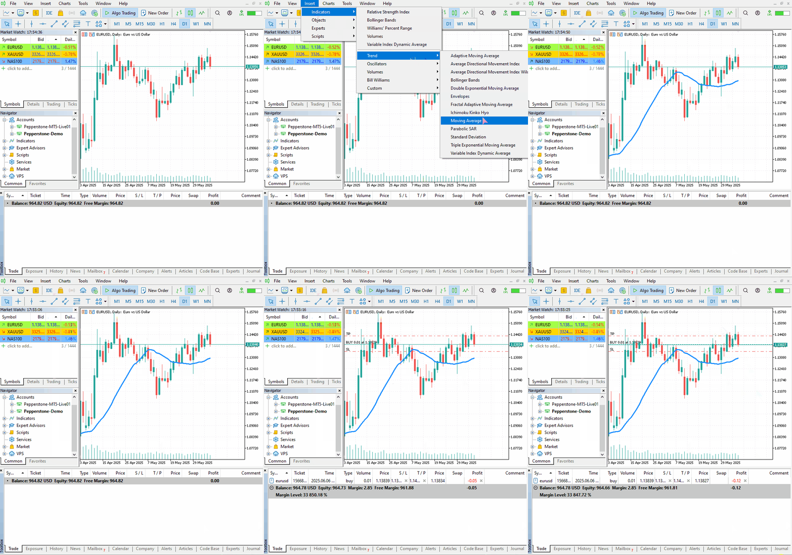
使用本文中讨论的交易类,我们检查是否存在同类型持仓;如果不存在,则开仓同类型持仓。预测值 high_open 和 open_low 分别用于设置买入交易的止盈和止损,卖出交易则相反。
周期(窗口)= 20 的简单移动平均线指标用作确认信号。如果当前收盘价高于移动平均线指标,我们开买入交易;否则,我们做相反的操作,开卖出交易。
输出。
最后的思考
向量自回归是一个不错的经典时间序列模型,具备预测多个回归特征的能力,这是大多数机器学习模型所不具备的。
这些模型具有以下优点:
- 具有较灵活的滞后结构,
- 能够捕捉相互依赖关系(变量之间的动态关系),
- 没有严格的外生性假设,而这在传统回归模型中通常存在。
它们的一些缺点包括:
- 对平稳变量敏感,仅在平稳数据中效果最佳。
- 假设变量与其滞后项之间存在线性关系,这在金融市场中并不总是成立。
- 当变量和滞后项较多时,也可能出现过拟合问题。
本文旨在提高人们对该模型、其构成以及如何应用于交易数据的认识,因为我发现网上关于这个特定主题的文档较少。请随时改进这个想法以满足您的需求。
此致敬礼。
附件表格
| 文件名 | 描述与用途 |
|---|---|
| Trade/* | 使用 Python 编写、风格类似 MQL5 的交易类 |
| error_description.py | 包含 MetaTrader 5 错误代码描述 |
| forex-ts-forecasting-using-var.ipynb | 用于学习目的的 Jupyter 笔记本,包含示例 |
| VAR.py | 包含利用 VAR 模型进行训练和预测的类 |
| VAR-TradingRobot.py | 一个交易机器人,根据 VAR 模型的预测结果开买入和卖出交易 |
本文由MetaQuotes Ltd译自英文
原文地址: https://www.mql5.com/en/articles/18371
注意: MetaQuotes Ltd.将保留所有关于这些材料的权利。全部或部分复制或者转载这些材料将被禁止。
本文由网站的一位用户撰写,反映了他们的个人观点。MetaQuotes Ltd 不对所提供信息的准确性负责,也不对因使用所述解决方案、策略或建议而产生的任何后果负责。


 MQL5中的自优化智能交易系统(第十一部分):线性代数基础入门
 神经网络在交易中的应用:基于自适应模态分解的时间序列预测(终篇)
 神经网络在交易中的应用:基于自适应模态分解(ACEFormer)的时间序列预测
