

Processos gaussianos em machine learning (Parte 2): Implementação e teste do modelo de classificação em MQL5
 249
249
 4
4

Introdução
No artigo anterior, apresentamos os fundamentos teóricos do modelo bayesiano de machine learning, os processos gaussianos (PG), e também iniciamos o desenvolvimento da biblioteca de PG em MQL5, descrevendo duas classes-chave: GaussianProcess e GPOptimizationObjective.
Hoje concluiremos o desenvolvimento da biblioteca, analisando em detalhes a implementação das interfaces-chave: IKernel, ILikelihood e IInference. Depois disso, testaremos a biblioteca com dados sintéticos e escreveremos indicadores para classificação e regressão, que mostrem sua operação em modo online, com o modelo sendo retreinado a cada nova barra.
Interface IKernel
A interface IKernel, que você encontrará no arquivo Kernels.mqh, é a base para a criação de kernels de covariância em nossa biblioteca. Ela torna o sistema flexível e fácil de estender, pois permite adicionar novos tipos de kernels ou suas combinações sem alterar a estrutura principal do código.
interface IKernel { // Calculate the covariance matrix between two data sets virtual matrix Compute(const matrix &X1, const matrix &X2) = 0; // Calculate the derivative of the covariance matrix with respect to the given hyperparameter // param_index: index of the hyperparameter by which the derivative is taken (starting from 0) virtual matrix ComputeDerivative(int param_index) = 0; // Return the current values of all kernel hyperparameters virtual vector GetHyperparameters() const = 0; // Set new values for kernel hyperparameters virtual void SetHyperparameters(const vector ¶ms) = 0; // Return the number of kernel hyperparameters virtual int GetNumHyperparameters() const = 0; // Return the kernel string name virtual string GetName() const = 0; };
A interface define os dois métodos mais importantes que sustentam o funcionamento de qualquer kernel:
- Compute(const matrix &X1, const matrix &X2): calcula a matriz de covariância K entre dois conjuntos de dados.
- ComputeDerivative(int param_index): calcula a derivada da matriz de covariância em relação a um dos hiperparâmetros do kernel. O param_index indica o índice do hiperparâmetro em relação ao qual a derivada é obtida.
Classe RBFKernel (Kernel de base radial)
RBFKernel, também conhecido como kernel gaussiano ou exponencial quadrático, é um dos kernels de covariância mais usados. Ele tem dois hiperparâmetros: a variância do sinal σ_f (amplitude) e a escala de comprimento l (length), que determina a suavidade da função.
//+------------------------------------------------------------------+ //| Kernel RBF class | //+------------------------------------------------------------------+ class RBFKernel : public IKernel { private: double length; double sigma_f; int n; // Number of rows in X1; int m; // Number of rows in X2; matrix m_K; matrix m_D_sq; // matrix of squared distances ||x_i - x_j||^2 public: //Constructor RBFKernel(double ls, double sf) : length(ls), sigma_f(sf) {} //Destructor ~RBFKernel() {} matrix Compute(const matrix &X1, const matrix &X2) override { n = (int)X1.Rows(); m = (int)X2.Rows(); matrix XX(n, m); if (!XX.GeMM(X1, X2.Transpose(), 1.0, 0.0)) { Print("Error: Failed to calculate XX = X * X^T"); return matrix::Zeros(n, m); } matrix diag1(n, 1); matrix X1_sq = X1 @ X1.Transpose(); diag1.Col(X1_sq.Diag(), 0); matrix diag2(m, 1); matrix X2_sq = X2 @ X2.Transpose(); diag2.Col(X2_sq.Diag(), 0); m_D_sq = matrix::Ones(n, 1) @ diag2.Transpose() + diag1 @ matrix::Ones(1, m) - 2 * XX; m_K = sigma_f * sigma_f * MathExp((-1 * m_D_sq) / (2 * length * length)); return m_K; } matrix ComputeDerivative(int param_index) override { matrix dK(n, m); switch (param_index) { case 0: { dK = (2.0 / sigma_f) * m_K; break; } case 1: { dK = m_K * (m_D_sq / (length * length * length)); break; } } return dK; } vector GetHyperparameters() const override { vector params(2); params[0] = sigma_f; params[1] = length; return params; } void SetHyperparameters(const vector ¶ms) override { if (params.Size() == 2) { sigma_f = params[0]; length = params[1]; } } int GetNumHyperparameters() const override { return 2; } string GetName() const override { return "RBFKernel"; } };
Felizmente, para o kernel RBF, as derivadas são fáceis de obter:
-
Derivada em relação a sigma_f:

- Derivada em relação a l:

Para o parâmetro length, multiplicamos a matriz K elemento a elemento por (D_sq / length^3), sendo D_sq a matriz dos quadrados das distâncias euclidianas.
Classe LinearKernel (Kernel linear)
LinearKernel é um kernel de covariância simples que pressupõe uma dependência linear entre os pontos de dados. Ele é frequentemente aplicado quando se espera que a função seja aproximável por um modelo linear, ou como componente em kernels compostos mais complexos.
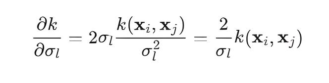
O kernel linear possui um hiperparâmetro: a variância do sinal σ_l.
//+------------------------------------------------------------------+ //| Linear kernel class | //+------------------------------------------------------------------+ class LinearKernel : public IKernel { private: double sigma_l; int n; int m; matrix m_K; public: //Constructor LinearKernel(double sl): sigma_l(sl){} //Destructor ~LinearKernel() {} matrix Compute(const matrix &X1, const matrix &X2) override { n = (int)X1.Rows(); m = (int)X2.Rows(); m_K.GeMM(X1, X2.Transpose(), sigma_l * sigma_l, 0.0); return m_K; } matrix ComputeDerivative(int param_index) override { matrix dK(n, m); switch (param_index) { case 0: { // Derivative with respect to sigma_l dK = (2.0 / sigma_l) * m_K; break; } } return dK; } vector GetHyperparameters() const override { vector params(1); params[0] = sigma_l; return params; } void SetHyperparameters(const vector ¶ms) override { if (params.Size() == 1) { sigma_l = params[0]; } } int GetNumHyperparameters() const override { return 1; } string GetName() const override { return "LinearKernel"; } };
Método ComputeDerivative(int param_index):
Classe PeriodicKernel (Kernel periódico)
PeriodicKernel é usado para modelar dados com padrões repetitivos ou sazonalidade, permitindo captar dependências cíclicas.
//+------------------------------------------------------------------+ //| Periodic kernel class | //+------------------------------------------------------------------+ class PeriodicKernel : public IKernel { private: double sigma_f; // Signal variance (oscillation amplitude) double length; // Scale length (smoothness of oscillations) double period; // Oscillation period int n; // Number of rows in X1 int m; // Number of rows in X2 matrix m_K; // Covariance matrix matrix m_D; // D matrix (sum of derivatives with respect to d [2 * sin^2(M_PI*distance/period] ) matrix m_distance_dim[]; // Array of difference matrices for each dimension |x_i_k - x_j_k| int m_d_cols; // Number of dimensions (features) (X.Cols()) public: //Constructor PeriodicKernel(double ls, double sf, double p) : sigma_f(sf), length(ls), period(p){} //Destructor ~PeriodicKernel() {} matrix Compute(const matrix &X1, const matrix &X2) override { n = (int)X1.Rows(); m = (int)X2.Rows(); int d = (int)X1.Cols(); m_d_cols = d; m_D = matrix::Zeros(n, m); ArrayResize(m_distance_dim, d); for (int k = 0; k < d; k++) { vector x1_k = X1.Col(k); vector x2_k = X2.Col(k); // Create a matrix where each column is a x1_k vector // (n x 1) * (1 x m) = (n x m) matrix x1_k_copy = x1_k.Outer(vector::Ones(m)) ; // Create a matrix where each row is the transposed vector of x2_k // (n x 1) * (1 x m) = (n x m) matrix x2_k_copy = vector::Ones(n).Outer(x2_k); // Calculate the matrix of all pairwise absolute differences between the elements of vectors x1_k and x2_k matrix distance = MathAbs(x1_k_copy - x2_k_copy); m_distance_dim[k] = distance; // Cache 'distance' for each dimension (feature) matrix sin_term = MathSin(M_PI * distance / period); sin_term = 2.0 * sin_term * sin_term; // 2 * sin^2(u) m_D += sin_term; // Sum up element by element } // Calculate the K matrix m_K = sigma_f * sigma_f * MathExp(-1 * m_D / (length * length)); return m_K; } matrix ComputeDerivative( int param_index) override { matrix dK(n, m); switch (param_index) { case 0: { // Derivative with respect to sigma_f // dK/d(sigma_f) = (2 / sigma_f) * K dK = (2.0 / sigma_f) * m_K; break; } case 1: { // Derivative with respect to 'length' // dK/d(length) = K * (2 * D / length^3) dK = m_K * ( 2.0 * m_D / (length * length * length) ); break; } case 2: { // Derivative with respect to 'period' // dK/d(period) = K * (-1/l^2) * dD/d(period) // dD/d(period) = Sum{k=1:d} (2 * pi * (x_ik - x_jk) / period^2) * sin(2*pi*(x_ik - x_jk)/period) matrix dD_dp = matrix::Zeros(n, m); for (int k = 0; k < m_d_cols; k++) { // Loop through each dimension (column) of the data matrix distance_k = m_distance_dim[k]; // matrix of absolute differences for the k-th dimension matrix u = M_PI * distance_k / period; // Calculate the argument u_k = pi * |x_ik - x_jk| / period matrix sin_2u = MathSin(2.0 * u); // Calculate sin(2 * u_k) // Use the already calculated u to calculate // -pi * |x_ik - x_jk| / period^2 matrix second_term = (-1*u) / period; // Accumulate dD/d(period) for the current measurement dD_dp += 2.0 * sin_2u * second_term; } // unite all parts of the derivative // dK = K * (-1/length^2) * dD_dp dK = m_K * (-1.0 / (length * length)) * dD_dp; break; } } return dK; } vector GetHyperparameters() const override { vector params(3); params[0] = sigma_f; params[1] = length; params[2] = period; return params; } void SetHyperparameters(const vector ¶ms) override { if (params.Size() == 3) { sigma_f = params[0]; length = params[1]; period = params[2]; } } int GetNumHyperparameters() const override { return 3; } string GetName() const override { return "PeriodicKernel"; } };
Derivada do kernel periódico em relação ao parâmetro period:
O cálculo da derivada em relação ao parâmetro period é o mais complexo, pois period está dentro de uma função trigonométrica, que, por sua vez, faz parte da exponencial.
A fórmula da derivada se baseia na regra da cadeia, em que K depende de D, e D depende de period por meio dos termos senoidais. A implementação de ComputeDerivative calcula iterativamente o termo dD_dp para cada dimensão e, em seguida, obtém a derivada resultante:
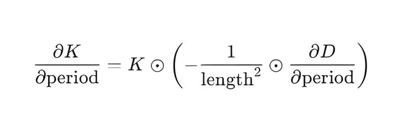
em que dD_dp é calculado como a soma das derivadas de 2 * sin^2(M_PI*distance/period) em todas as dimensões (atributos).
Kernels compostos
Os processos gaussianos permitem combinar kernels de covariância simples para construir modelos mais complexos, capazes de descrever diferentes aspectos dos dados (por exemplo, tendência, periodicidade, ruído). Essa funcionalidade usa dois kernels compostos:
- SumKernel: combina vários kernels somando suas matrizes de covariância.
- ProductKernel: combina kernels multiplicando suas matrizes de covariância elemento a elemento.
Ambas as classes gerenciam os hiperparâmetros de seus kernels filhos, reunindo-os em um único vetor para otimização e, em seguida, distribuindo-os de volta para os kernels filhos.
Classe SumKernel
//+------------------------------------------------------------------+ //| Class for the sum of kernels | //+------------------------------------------------------------------+ class SumKernel : public IKernel { private: IKernel* kernels[]; public: // Constructor SumKernel(IKernel* &input_kernels[]) { ArrayResize(kernels, ArraySize(input_kernels)); ArrayCopy(kernels, input_kernels); } //Destructor ~SumKernel() { for (int i = 0; i < ArraySize(kernels); i++) { if (kernels[i] != NULL) { delete kernels[i]; } } ArrayFree(kernels); } matrix Compute(const matrix &X1, const matrix &X2) override { int n = (int)X1.Rows(); int m = (int)X2.Rows(); matrix sum = matrix::Zeros(n,m); for (int i = 0; i < ArraySize(kernels); i++) { sum += kernels[i].Compute(X1, X2); // Sum the matrices from each child kernel } return sum; } matrix ComputeDerivative(int param_index) override { int current_param_offset = 0; // Start at offset 0 for the first kernel for (int i = 0; i < ArraySize(kernels); i++) { // Get the number of hyperparameters of the current child kernel int num_params_current_kernel = kernels[i].GetNumHyperparameters(); // Check if the global param_index belongs to the current child kernel // param_index should be: // - greater than or equal to the current offset // - strictly less than the current offset + the number of parameters of the current kernel if (param_index >= current_param_offset && param_index < current_param_offset + num_params_current_kernel) { // If param_index belongs to this kernel, calculate its local index int local_param_index = param_index - current_param_offset; // Call ComputeDerivative on the found child kernel and // pass it the local index. // Since the derivative of the sum of kernels with respect to the parameter of one kernel is equal to the derivative // of this particular kernel by this parameter, we can immediately return the result return kernels[i].ComputeDerivative(local_param_index); } // If param_index does not belong to the current kernel, // increase the offset to check the next kernel current_param_offset += num_params_current_kernel; } Print("Error: SumKernel::ComputeDerivative - Parameter index ", param_index, " out of bounds"); return matrix::Zeros(1, 1); } //+---------------------------------------------------------------------------------+ //| The function returns the values of all hyperparameters of the composite kernel | //+---------------------------------------------------------------------------------+ vector GetHyperparameters() const override { vector all_params(GetNumHyperparameters()); int current_idx = 0; for (int i = 0; i < ArraySize(kernels); i++) { // Get the values of the parameters of the current child kernel vector kernel_params = kernels[i].GetHyperparameters(); for (int j = 0; j < (int)kernel_params.Size(); j++) { // Copy the parameters into the common vector all_params[current_idx + j] = kernel_params[j]; } // Update the offset for the next kernel current_idx += (int)kernel_params.Size(); } return all_params; } //+----------------------------------------------------------------------+ //|The function takes a vector of values of all hyperparameters, breaks | //|it into the appropriate parts and assigns them to each child kernel | //+----------------------------------------------------------------------+ void SetHyperparameters(const vector ¶ms) override { int current_idx = 0; for (int i = 0; i < ArraySize(kernels); i++) { // Get the number of hyperparameters of the current child kernel int num_params = kernels[i].GetNumHyperparameters(); vector sub_params(num_params); // Copy the corresponding parameters from the general vector for (int j = 0; j < num_params; j++) { sub_params[j] = params[current_idx + j]; } // Call the SetHyperparameters() method on the current child kernel, // passing it only its own parameters, collected in the sub_params vector kernels[i].SetHyperparameters(sub_params); current_idx += num_params; } } //+---------------------------------------------------------------------------------------+ //| Returns the total number of hyperparameters for the entire SumKernel composite kernel | //+---------------------------------------------------------------------------------------+ int GetNumHyperparameters() const override { int total_params = 0; for (int i = 0; i < ArraySize(kernels); i++) { total_params += kernels[i].GetNumHyperparameters(); } return total_params; } string GetName() const override { string name = "Sum("; for (int i = 0; i < ArraySize(kernels); i++) { name += kernels[i].GetName(); if (i < ArraySize(kernels) - 1) name += ","; } name += ")"; return name; } //+------------------------------------------------------------------+ //| Provide external access to the list of child kernels | //+------------------------------------------------------------------+ void GetKernels(IKernel* &output_kernels[]) const { // Copy pointers from the internal kernels array to the passed // output_kernels external array. This provides access to child // kernels in the GaussianProcess::Fit() method, where it is necessary to iterate through // all elementary kernels to set optimization boundaries // of their hyperparameters. ArrayCopy(output_kernels, kernels); } };
- Método Compute: calcula a matriz de covariância final K como uma soma simples das matrizes de covariância retornadas por cada kernel filho. Aqui, aplica-se o princípio do polimorfismo: embora o array kernels armazene ponteiros do tipo base IKernel*, a chamada kernels[i].Compute(X1, X2), na prática, chama a implementação específica de Compute para cada kernel filho concreto. Isso permite que SumKernel trabalhe com qualquer kernel herdado de IKernel.
- Método ComputeDerivative: a derivada da função de covariância da soma de kernels em relação a um hiperparâmetro específico corresponde à derivada da função de covariância somente do kernel filho ao qual esse hiperparâmetro pertence. Isso significa que ComputeDerivative encontra o kernel filho correspondente por param_index e retorna somente sua derivada. As derivadas em relação aos parâmetros dos demais kernels filhos são consideradas iguais a zero.
Classe ProductKernel
//+------------------------------------------------------------------+ //| Class for the product of kernels | //+------------------------------------------------------------------+ class ProductKernel : public IKernel { private: IKernel* kernels[]; matrix m_X1; matrix m_X2; int n; int m; public: // Constructor: copies pointers to child kernels ProductKernel(IKernel* &input_kernels[]) { ArrayResize(kernels, ArraySize(input_kernels)); ArrayCopy(kernels, input_kernels); } // Destructor ~ProductKernel() { for (int i = 0; i < ArraySize(kernels); i++) { if (kernels[i] != NULL){ delete kernels[i]; } } ArrayFree(kernels); } matrix Compute(const matrix &X1, const matrix &X2) override { n = (int)X1.Rows(); m = (int)X2.Rows(); m_X1 = X1; m_X2 = X2; matrix product = matrix:: Ones(n,m); for (int i = 0; i < ArraySize(kernels); i++) { // Polymorphism: call the Compute() method of each child kernel, // regardless of its specific type, and multiply the result element by element product *= kernels[i].Compute(X1, X2); } return product; } matrix ComputeDerivative(int param_index) override { matrix dK_prod(n, m); // Final derivative matrix int current_param_offset = 0; int target_kernel_idx = -1; // Kernel index the hyperparameter belongs to int local_param_index = -1; // Local index of the hyperparameter in this kernel // Step 1: Find the kernel and local index of the hyperparameter for (int i = 0; i < ArraySize(kernels); i++) { int num_params_current_kernel = kernels[i].GetNumHyperparameters(); if (param_index >= current_param_offset && param_index < current_param_offset + num_params_current_kernel) { target_kernel_idx = i; local_param_index = param_index - current_param_offset; break; } current_param_offset += num_params_current_kernel; } if (target_kernel_idx == -1) { Print("Error: ProductKernel::ComputeDerivative - Parameter index ", param_index, " out of bounds"); return matrix::Zeros(1, 1); } // Step 2: Calculate dK_k / d_theta_j for the target kernel matrix dK_target_kernel = kernels[target_kernel_idx].ComputeDerivative(local_param_index); // Step 3: Calculate the K_m product for all other kernels (m != k) matrix other_kernels_product = matrix::Ones(n, m); for (int i = 0; i < ArraySize(kernels); i++) { if (i != target_kernel_idx) { // Skip the target kernel other_kernels_product = other_kernels_product * kernels[i].Compute(m_X1, m_X2); } } // Step 4: Multiply the results element by element dK_prod = dK_target_kernel * other_kernels_product; return dK_prod; } // Collect the hyperparameter values of all child kernels into a single vector vector GetHyperparameters() const override { vector all_params(GetNumHyperparameters()); int current_idx = 0; for (int i = 0; i < ArraySize(kernels); i++) { vector kernel_params = kernels[i].GetHyperparameters(); for (int j = 0; j < (int)kernel_params.Size(); j++) { all_params[current_idx + j] = kernel_params[j]; } current_idx += (int)kernel_params.Size(); } return all_params; } void SetHyperparameters(const vector ¶ms) override { int current_idx = 0; for (int i = 0; i < ArraySize(kernels); i++) { int num_params_kernel = kernels[i].GetNumHyperparameters(); vector sub_params(num_params_kernel); for (int j = 0; j < num_params_kernel; j++) { sub_params[j] = params[current_idx + j]; } kernels[i].SetHyperparameters(sub_params); current_idx += num_params_kernel; } } int GetNumHyperparameters() const override { int total_params = 0; for (int i = 0; i < ArraySize(kernels); i++) { total_params += kernels[i].GetNumHyperparameters(); } return total_params; } string GetName() const override { string name = "Prod("; for (int i = 0; i < ArraySize(kernels); i++) { name += kernels[i].GetName(); if (i < ArraySize(kernels) - 1) name += "*"; } name += ")"; return name; } //+------------------------------------------------------------------+ //| Provide external access to the list of child kernels | //+------------------------------------------------------------------+ void GetKernels(IKernel* &output_kernels[]) const { ArrayCopy(output_kernels, kernels); } };
- Método Compute: calcula a matriz de covariância final K como o produto elemento a elemento das matrizes de covariância retornadas por cada kernel filho. Assim como em SumKernel, aqui o polimorfismo é usado para chamar o método Compute do kernel filho correspondente.
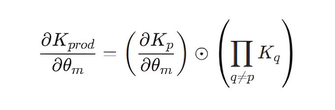
- Método ComputeDerivative: para calcular a derivada de K em relação ao hiperparâmetro pertencente a um kernel filho específico, K_p, ProductKernel aplica a regra do produto (regra de Leibniz). A derivada de K em relação a esse parâmetro é igual à derivada da matriz K_p em relação a esse parâmetro, multiplicada pelo produto elemento a elemento das matrizes de covariância de todos os demais kernels filhos, sem derivar:
Interface ILikelihood
A interface ILikelihood define como qualquer função de verossimilhança deve operar em nossa biblioteca. Ela nos permite trabalhar com diferentes tipos de dados, tanto com valores contínuos (como na regressão) quanto com categorias discretas (como na classificação).
//+------------------------------------------------------------------+ //|Interface for likelihood functions | //+------------------------------------------------------------------+ interface ILikelihood { // Compute the p(y|f) log-likelihood for latent values f and observed values y virtual double LogLikelihood(const vector &f, const vector &y) = 0; //----------------------------- Derivatives of the logarithm of the likelihood with respect to f ----------------- // Calculate the vector of the first derivative of the log-likelihood with respect to f (dlp/df) virtual vector LogLikelihoodGradient(const vector &f, const vector &y) = 0; // Compute the second derivative (Hessian) matrix of the log-likelihood with respect to f (d^2lp/df df^T) virtual matrix LogLikelihoodHessian(const vector &f, const vector &y) = 0; // Calculate the vector of the third derivative of the log-likelihood with respect to f (d^3lp/df^3) virtual vector LogLikelihoodThirdDerivative(const vector &f, const vector &y) = 0; //----------------------------- Derivatives of the logarithm of the likelihood with respect to the parameters ----------------- // The first derivative of the log-likelihood with respect to the j-th likelihood hyperparameter. virtual double LogLikelihoodGradientParam(const vector &f, const vector &y, int param_index) = 0; // Hessian derivative of the log-likelihood with respect to the j-th likelihood hyperparameter. virtual matrix LogLikelihoodHessianDerivative(const vector &f, const vector &y, int param_index) = 0; // Return the name of the likelihood function virtual string GetName() const = 0; // Return the current values of the likelihood hyperparameters virtual vector GetHyperparameters() const = 0; // Set new values for the likelihood hyperparameters virtual void SetHyperparameters(const vector ¶ms) = 0; // Return the number of likelihood hyperparameters virtual int GetNumHyperparameters() const = 0; };
Classe GaussianLikelihood
GaussianLikelihood implementa a função de verossimilhança para tarefas de regressão, assumindo ruído normal nos dados observados.
//+------------------------------------------------------------------+ //| Gaussian likelihood class (for regression problems) | //+------------------------------------------------------------------+ class GaussianLikelihood : public ILikelihood { private: double m_noise_sigma; // Noise parameter (standard deviation) public: // Constructor GaussianLikelihood(double initial_noise_sigma) : m_noise_sigma(initial_noise_sigma) {} // Return the current value of the hyperparameter vector GetHyperparameters() const override { vector params(1); params[0] = m_noise_sigma; return params; } // Set a new hyperparameter value void SetHyperparameters(const vector ¶ms) override { if (params.Size() == 1) { m_noise_sigma = params[0]; } } // Return the number of hyperparameters int GetNumHyperparameters() const override { return 1; } // Calculate the log p(y|f) log-likelihood for a Gaussian distribution double LogLikelihood(const vector &f, const vector &y) override { int n = (int)y.Size(); double noise_variance = m_noise_sigma * m_noise_sigma; vector residual = y - f; // Formula for the logarithm of the density of a multivariate normal distribution return -0.5 / noise_variance * (residual @ residual) - 0.5 * n * MathLog(2 * M_PI * noise_variance); } //------------------ Derivatives with respect to f ----------------------- // Calculate the vector of the first derivative of the log-likelihood with respect to f (dlp/df) vector LogLikelihoodGradient(const vector &f, const vector &y) override { // d(log p(y|f))/df = (y - f) / sigma^2 return (y - f) / (m_noise_sigma * m_noise_sigma); } // Compute the second derivative (Hessian) matrix of the log-likelihood with respect to f (d^2lp/dfdf^T) matrix LogLikelihoodHessian(const vector &f, const vector &y) override { // d^2(log p(y|f))/dfdf^T = -1/sigma^2 * I int n = (int)y.Size(); return matrix::Identity(n, n) * (-1.0 / (m_noise_sigma * m_noise_sigma)); } // Calculate the vector of the third derivative of the log-likelihood with respect to f vector LogLikelihoodThirdDerivative(const vector &f, const vector &y) override { // For Gaussian likelihood d^3(log p(y|f))/df^3 = 0 return vector::Zeros((int)y.Size()); } // ------------------------------ Derivatives with respect to the parameter ----------------------------------- // // Calculate the first derivative of the log-likelihood with respect to the j-th likelihood hyperparameter virtual double LogLikelihoodGradientParam(const vector &f, const vector &y, int param_index) override { // Gaussian likelihood has only 1 hyperparameter: m_noise_sigma (index 0) if (param_index == 0) { // Formula for d(log p(y|f))/d(sigma_n): // = (y-f)^T(y-f) / sigma_n^3 - N / sigma_n vector y_minus_f = y - f; double sn3 = m_noise_sigma * m_noise_sigma * m_noise_sigma; double term1 = (y_minus_f @ y_minus_f) / sn3; double term2 = y.Size() / m_noise_sigma; // N / sigma_n return term1 - term2; } else { return 0.0; } } // Calculate the Hessian derivative of the log-likelihood with respect to the j-th likelihood hyperparameter matrix LogLikelihoodHessianDerivative(const vector &f, const vector &y, int param_index) override { int n = (int)y.Size(); if (param_index == 0) { // Derivative of Hessian with respect to m_noise_sigma: d/d(sigma_n) [-1/sigma_n^2 * I] = (2/sigma_n^3) * I double derivative_coeff = 2.0 / (m_noise_sigma * m_noise_sigma * m_noise_sigma); return matrix::Identity(n, n) * derivative_coeff; } else { return matrix::Zeros(n, n); } } string GetName() const override { return "GaussianLikelihood"; } };
Métodos principais:
- Construtor GaussianLikelihood: inicializa o único hiperparâmetro, o desvio padrão do ruído.
- LogLikelihood(): calcula o logaritmo da verossimilhança p(y∣f) para a densidade de probabilidade da distribuição normal multivariada:

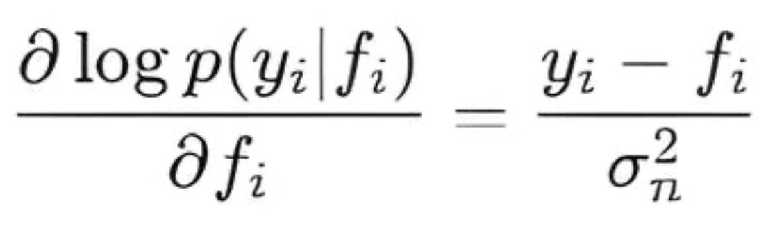
- LogLikelihoodGradient(): calcula a primeira derivada do logaritmo da verossimilhança em relação aos valores latentes f. É um vetor em que cada elemento é igual a:
- LogLikelihoodHessian(): calcula a segunda derivada (Hessiano) do logaritmo da verossimilhança em relação a f. Para a verossimilhança gaussiana, a matriz Hessiana é diagonal:
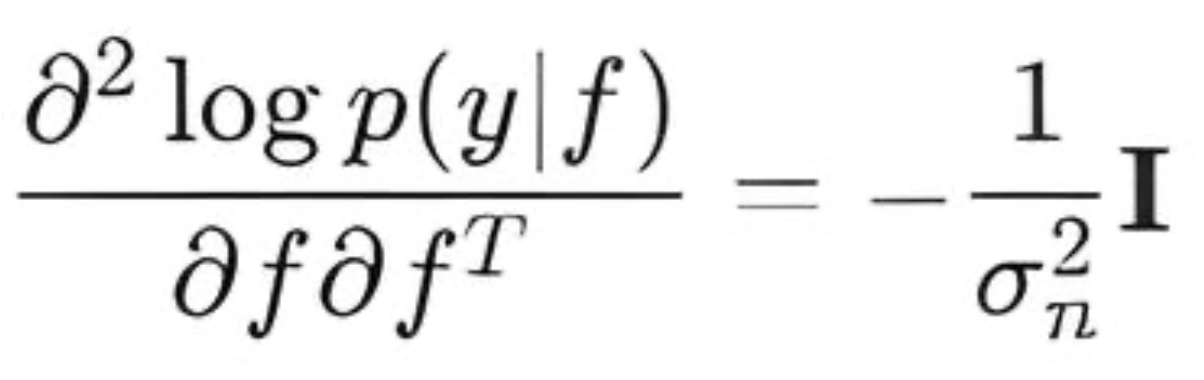
- LogLikelihoodThirdDerivative(): calcula a terceira derivada. Para a verossimilhança gaussiana, todas as derivadas de ordem superior à segunda são iguais a zero.
- LogLikelihoodGradientParam(): calcula a primeira derivada do logaritmo da verossimilhança em relação ao hiperparâmetro m_noise_sigma:
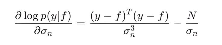
- LogLikelihoodHessianDerivative(): calcula a derivada da Hessiana do logaritmo da verossimilhança em relação ao hiperparâmetro m_noise_sigma:
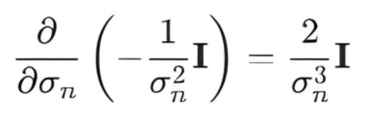
Classe LogitLikelihood
LogitLikelihood é usada para classificação binária, em que os valores-alvo observados y assumem os valores {−1,+1}. Essa função relaciona a função latente f à probabilidade de pertencimento a uma classe via função sigmoide.
A implementação de LogitLikelihood inclui as funções auxiliares sigmoid() e Softplus(), com tratamento de valores de entrada muito grandes ou muito pequenos.
//+------------------------------------------------------------------+ //| Class for Logit likelihood (y {-1, +1}) | //+------------------------------------------------------------------+ class LogitLikelihood : public ILikelihood { public: // logit_sigmoid(x) = 1 / (1 + exp(-x)) double sigmoid(double x) const { if (x > 100.0) return 1.0; // Avoid NaN occurrences if (x < -100.0) return 0.0; return 1.0 / (1.0 + MathExp(-x)); } // Softplus log(1 + exp(x)) function double Softplus(double x) const { if (x > 100.0) return x; // For very large x, log(1 + exp(x)) ~ x if (x < -100.0) return MathExp(x); // For very small x, log(1 + exp(x)) ~ exp(x) return MathLog(1.0 + MathExp(x)); } public: // Constructor (logit likelihood has no hyperparameters of its own) LogitLikelihood() {} vector GetHyperparameters() const override { return vector::Zeros(0); } void SetHyperparameters(const vector ¶ms) override {} // Return the number of likelihood hyperparameters int GetNumHyperparameters() const override { return 0; } // --- Calculate the log-likelihood: log p(y|f) --- // Formula: sum_i (-log(1 + exp(-y_i * f_i))) double LogLikelihood(const vector &f, const vector &y) override { int n = (int)y.Size(); double total_log_likelihood = 0.0; for (int i = 0; i < n; i++) { total_log_likelihood += -Softplus(-y[i] * f[i]); } return total_log_likelihood; } // Compute the gradient of the log-likelihood with respect to f // Formula: d(log p(y_i|f_i))/df_i = y_i * sigma(-y_i * f_i) vector LogLikelihoodGradient(const vector &f, const vector &y) override { int n = (int)y.Size(); vector grad(n); for (int i = 0; i < n; i++) { grad[i] = y[i] * sigmoid(-y[i] * f[i]); // grad[i] = y[i] * (1 - sigmoid(y[i] * f[i])); equivalent to } return grad; } // Compute the Hessian of the log-likelihood of f (the H diagonal matrix) // Formula: d^2(log p(y_i|f_i))/df_i^2 = -sigma(y_i*f_i)(1 - sigma(y_i*f_i)) matrix LogLikelihoodHessian(const vector &f, const vector &y) override { int n = (int)y.Size(); matrix H = matrix::Identity(n, n); for (int i = 0; i < n; i++) { double sig = sigmoid(y[i] * f[i]); H[i][i] = -1*sig * (1.0 - sig); } return H; } // Calculate the third derivative of the log-likelihood with respect to f // Formula: d^3(log p(y_i|f_i))/df_i^3 = y_i * sigma(-y_i f_i) * (1 - sigma(-y_i f_i)) * (1 - 2*sigma(-y_i f_i)) vector LogLikelihoodThirdDerivative(const vector &f, const vector &y) override { int n = (int)y.Size(); vector third_deriv(n); for (int i = 0; i < n; i++) { double sig_neg_yf = sigmoid(-y[i] * f[i]); third_deriv[i] = y[i] * sig_neg_yf * (1.0 - sig_neg_yf) * (1.0 - 2.0 * sig_neg_yf); // equivalent to // double sig_yf = sigmoid(y[i] * f[i]); // third_deriv[i] = -y[i] * sig_yf * (1.0 - sig_yf) * (1.0 - 2.0 * sig_yf); } return third_deriv; } // LogitLikelihood has no hyperparameters virtual double LogLikelihoodGradientParam(const vector &f, const vector &y, int param_index) override { return 0.0; } // LogitLikelihood has no hyperparameters matrix LogLikelihoodHessianDerivative(const vector &f_latent, const vector &y, int param_index) override { int n = (int)y.Size(); return matrix::Zeros(n, n); } string GetName() const override { return "LogitLikelihood"; } };
Métodos principais:
- LogLikelihood(): calcula o logaritmo da verossimilhança logp(y∣f). Para classificação binária com y em {−1,+1}, isso corresponde à soma dos logaritmos da verossimilhança de entropia cruzada binária:

- LogLikelihoodGradient(): calcula a primeira derivada do logaritmo da verossimilhança em relação a f. Cada elemento do vetor gradiente é igual a:
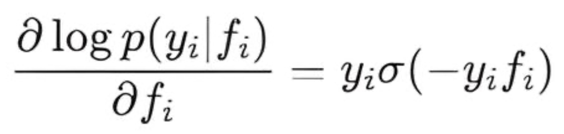
- LogLikelihoodHessian(): calcula a segunda derivada (Hessiana) do logaritmo da verossimilhança em relação a f. Para LogitLikelihood, a matriz Hessiana é diagonal cujos elementos diagonais são iguais a:
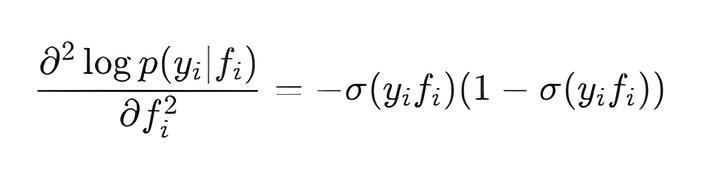
- LogLikelihoodThirdDerivative(): calcula a terceira derivada do logaritmo da verossimilhança em relação a f. Cada elemento do vetor é igual a:

Funções e estruturas auxiliares
O arquivo StructUtils.mqh contém um conjunto de enumerações, estruturas de dados e funções que facilitam a operação com PG.
    enum PredictMode {
    PROBIT      = 0,  // Probit Approximation
    NUM_INTEGR  = 1,  // Numerical integration
    MONTE_CARLO = 2   // Monte Carlo

};

//--- Structure for prediction results
struct GPPredictionResult
{
    vector mu_f_star;    // Posterior mean for the latent f* function on new data
    matrix Sigma_f_star; // Posterior covariance for the latent f* function on new data

    // Regression-only fields (GaussianLikelihood)
    vector mu_y_star;      // Posterior mean of observations y*
    matrix Sigma_y_star;   // Posterior covariance of observations y*

    // Fields for classification only (LogitLikelihood, ProbitLikelihood, etc.)
    vector predicted_probabilities; // Probabilities p(y*=+1 | X*, D)
    vector predicted_labels;        // Predicted y* labels (+1 or -1)
};

// Structure for the inference result
struct GPInferenceResult {
    double      nlml_value;    // Negative logarithm of the marginal likelihood
    vector      nlml_gradient; // NLML gradient by kernel and likelihood hyperparameters

    // Inference results on training data:
    vector      mu_f_train;    // Posterior mean of the latent function f on the training data
    matrix      Sigma_f_train; // Posterior covariance of the latent function f on the training data (K^−1+W)^−1
    matrix      L_K_noisy;     // Cholesky decomposition K_noisy = cholesky(K + s2n*I)
    matrix      L_B;           // Cholesky decomposition B = I + W^0.5 @ K @ W^0.5
    matrix      sW;            // sW = W^0.5;
    vector      sW_diag;       // sW diagonal
    matrix      sW_K;          // sW @ K
    vector      alpha;         // (K_noisy)^-1 * y
    matrix      H;             // Hessian of the log likelihood d^2 log p(y|f)/df^2 (for LaplaceInference)
    bool        success;       // Flag indicating success of the inference function
};
- A enumeração PredictMode define diferentes modos para executar previsões no modelo de classificação.
- A estrutura GPInferenceResult é usada para armazenar todos os resultados principais obtidos durante a inferência.
- A estrutura GPPredictionResult armazena todos os resultados obtidos após a previsão em novos dados de teste (X_test).
- DiagonalTrace
//+-------------------------------------------------------------------+
//| Compute the trace of the product of two matrices using only       |
//| diagonal elements of the final matrix                             |
//+-------------------------------------------------------------------+
double DiagonalTrace(const matrix &A, const matrix &B)
  {
   ulong m = A.Rows();
   ulong n = A.Cols();
   ulong n_b = B.Rows();
   ulong p = B.Cols();
// Find the minimum size for the diagonal
   ulong k = MathMin(m, p);
   double tr = 0.0;

   for(ulong i = 0; i < k; i++)
     {
      // Dot product of the i-th row of A and the i-th column of B
      tr += A.Row(i)@B.Col(i);
     }
   return tr;
  }
Calcula o traço do produto de duas matrizes A e B (Tr(A @ B)) sem precisar formar toda a matriz produto. Para isso, soma os produtos escalares das linhas da matriz A com as colunas correspondentes da matriz B. Essa abordagem permite reduzir significativamente o custo computacional em comparação com a multiplicação completa de matrizes.
- cho_solve (wrapper da OpenBLAS para LinearEquationsSolutionTriangular)
 //+-----------------------------------------------------------------------+
   //| Solve the system A*X = B using the Cholesky decomposition A = LL^T  |
   //| Parameters:                                                         |
   //|   c: Lower triangular matrix L from the Cholesky decomposition      |
   //|   b: right side of the system (matrix)                              |
   //| Return: matrix X - system solution                                  |
   //+---------------------------------------------------------------------+
   matrix            cho_solve(const matrix &c, const matrix &b)
     {
    // Check if 'c' matrix is lower triangular one
    if (!c.IsLowerTriangular()) {
        Print("Error: cho_solve - Input matrix 'c' is not lower triangular.");
        return matrix::Zeros(c.Rows(), b.Cols());
    }

// Step 1: Solve L * Y = B
    //  Y -  intermediate matrix, the result of solving L^-1 * B
    matrix Y;
    if (!c.LinearEquationsSolutionTriangular(EQUATIONSFORM_N, b, Y)) {
        PrintFormat("Error: cho_solve- LinearEquationsSolutionTriangular L * Y = B failed. Error Code: %d", GetLastError());
        return matrix::Zeros(c.Rows(), b.Cols());
    }

// Step 2: Solve L^T * X = Y
    //  X - L^T * X = Y system solution, which is equivalent to (L^T)^-1 * Y
    matrix X;
    if (!c.LinearEquationsSolutionTriangular(EQUATIONSFORM_T, Y, X)) {
        PrintFormat("Error: cho_solve- LinearEquationsSolutionTriangular L^T * X = Y failed. Error Code: %d", GetLastError());
        return matrix::Zeros(c.Rows(), b.Cols());
        }
      return X;
     }

   //+------------------------------------------------------------------+
   //| Solve the system Ax = b using the Cholesky decomposition A = LL^T|
   //| Parameters:                                                      |
   //|   c: Lower triangular matrix L from the Cholesky decomposition   |
   //|   b: right side of the system (vector)                           |
   //| Return: vector x - system solution                               |
   //+------------------------------------------------------------------+
   vector            cho_solve(const matrix &c, const vector &b)
     {
      // Check if 'c' matrix is lower triangular one
    if (!c.IsLowerTriangular()) {
        Print("Error: cho_solve - Input matrix 'c' is not lower triangular");
        return vector::Zeros(c.Rows());
    }

    // Step 1: Solve L * y = b
    // y - intermediate vector, the result of solving L^-1 * b
    vector y;
    if (!c.LinearEquationsSolutionTriangular(EQUATIONSFORM_N, b, y)) {
        PrintFormat("Error: cho_solve- LinearEquationsSolutionTriangular L * y = b failed. Error Code: %d", GetLastError());
        return vector::Zeros(c.Rows());
    }

    // Step 2: Solve L^T * x = y
    // x - final solution of the L^T * x = y system, which is equivalent to (L^T)^-1 * y
    vector x;
    if (!c.LinearEquationsSolutionTriangular(EQUATIONSFORM_T, y, x)) {
        PrintFormat("Error: cho_solve- LinearEquationsSolutionTriangular L^T * x = y failed. Error Code: %d", GetLastError());
        return vector::Zeros(c.Rows());
    }
      return x;
     }
A função cho_solve serve para resolver com eficiência sistemas de equações lineares Ax=b (ou AX=B quando B é uma matriz), em que a matriz A é obtida a partir de sua decomposição de Cholesky A=LL^T. Aqui, L é a matriz triangular inferior.
O cálculo direto de A^−1 (A.Inv()) exige muitos recursos e pode ser numericamente instável. A decomposição de Cholesky, por outro lado, oferece uma abordagem significativamente mais eficiente e confiável.
Em cho_solve, são executadas duas operações principais:
- Substituição progressiva: resolve-se o sistema LY=B (ou Ly=b), em que L é a matriz de entrada c e Y (ou y) é o resultado intermediário. Como L é uma matriz triangular, essa resolução é relativamente rápida.
- Substituição regressiva: em seguida, resolve-se o sistema L^TX=Y (ou L^Tx=y), em que L^T é a matriz transposta de L. Isso também é eficiente, pois L^T é uma matriz triangular superior.
Essas operações são implementadas com as funções LinearEquationsSolutionTriangular da biblioteca de álgebra linear de alto desempenho OpenBLAS. Também proporcionam uma aceleração significativa dos cálculos e se tornam indispensáveis para modelos de machine learning com alto consumo de recursos, como os processos gaussianos.
Interface IInference
interface IInference
  {
// This method performs inference (i.e., computes the posterior distribution of f)
// and returns the components needed for NLML and prediction
   virtual void Infer(const matrix &X, const vector &y,
                      IKernel *kernel, ILikelihood *likelihood,GPInferenceResult &result) = 0;
   virtual string GetName() const = 0;
  };
A interface permite alternar entre diferentes métodos de inferência, como a inferência exata para a verossimilhança gaussiana e métodos aproximados para casos não gaussianos, sem alterar a lógica central de GaussianProcess.
Infer é o método central desta interface. Ele executa a inferência da distribuição a posteriori da função latente f e retorna os componentes necessários para cálculos posteriores (NLML e previsões). Recebe os seguintes argumentos:
- X, matriz de atributos de treinamento,
- y, vetor de rótulos de treinamento,
- kernel, ponteiro para um objeto IKernel,
- likelihood, ponteiro para um objeto ILikelihood,
- result, referência à estrutura GPInferenceResult, usada para armazenar todos os resultados da inferência, incluindo:
- o logaritmo negativo da verossimilhança marginal (NLML), necessário para a otimização dos hiperparâmetros,
- o vetor de gradientes de NLML em relação a todos os hiperparâmetros do kernel e da verossimilhança,
- matrizes e vetores auxiliares: (L_K_noisy, L_B, sW, mu_f_train, Sigma_f_train, alpha), usados como suporte para calcular os gradientes de NLML e para a posterior previsão para novos dados.
Classe ExactInference
//+------------------------------------------------------------------+
//| ExactInference For Gaussian likelihood only                      |
//+------------------------------------------------------------------+
class ExactInference : public IInference
  {

public:
                     ExactInference() {}

   void              Infer(const matrix &X, const vector &y,
                           IKernel *kernel, ILikelihood *likelihood,GPInferenceResult &result) override
     {
      if(likelihood.GetName() != "GaussianLikelihood")
        {
         Print("ExactInference supports only GaussianLikelihood");
         result.nlml_value = DBL_MAX;
         return;
        }
      result.success = false;
      int n = (int)y.Size();

      //  Calculate K with current kernel parameters
      matrix K = kernel.Compute(X, X);

      //  Get the noise variance
      vector likelihood_params = likelihood.GetHyperparameters();
      double sigma = likelihood_params[0];
      double variance = sigma * sigma;

      double jitter = 1e-6;
      matrix K_noisy = K + matrix::Identity(n, n) * (variance + jitter);

      if(!K_noisy.Cholesky(result.L_K_noisy))
        {
         PrintFormat("Error: Cholesky decomposition failed. Error Code: %d",GetLastError());
         result.nlml_value = DBL_MAX;
         return;
        }
      //------------- Algorithm 2.1 GPML ---------------------------
      //Calculate alpha (K_noisy^-1 * y) - O(N^2)
      result.alpha = cho_solve(result.L_K_noisy, y);
      //+------------------------------------------------------------------+
      //| NLML = 0.5y^T(K+σ^2*I)^-1*y + 0.5*log|K+σ^2*I| +n/2*Log(2π)      |
      //+------------------------------------------------------------------+
      //+------------------------------------------------------------------+
      //| NLML = 0.5y^T*alpha         + 0.5*log|K+σ^2*I| +n/2*Log(2π)      |
      //+------------------------------------------------------------------+
      // --- Calculate the first term in the NLML equation:
      double data_term = 0.5 * (y @ result.alpha);
      // --- Calculate the second term: 1/2 * log|K + sigma^2*I| = sum(log(L_ii))
      double log_det = MathLog(result.L_K_noisy.Diag()).Sum();
      // --- Calculate the third term: n/2 * log(2π)
      double const_term = 0.5 * n * MathLog(2 * M_PI);
      //--- NLML
      result.nlml_value = data_term + log_det + const_term;

      // -------------------- NLML gradients calculations --------------------------------------
      result.nlml_gradient.Resize(kernel.GetNumHyperparameters() + likelihood.GetNumHyperparameters());
      int current_grad_idx = 0;
      // Calculate (K_noisy^-1)
      matrix K_noisy_inv = cho_solve(result.L_K_noisy, matrix::Identity(n, n));

      // 1. Gradients on kernel hyperparameters
      vector kernel_hyperparams = kernel.GetHyperparameters();
      // Calculate aatK_noisy_inv once before the loop - O(N^2)
      matrix aatK_noisy_inv = result.alpha.Outer(result.alpha) - K_noisy_inv;
      matrix dK_dtheta;
      for(int i = 0; i < (int)kernel_hyperparams.Size(); i++)
        {
         dK_dtheta = kernel.ComputeDerivative(i); // O(N^2)
         result.nlml_gradient[current_grad_idx] = -0.5 * DiagonalTrace(aatK_noisy_inv, dK_dtheta);
         current_grad_idx++;
        }
      // 2. Gradient over noise hyperparameter
      // dNLML/d(sigma^2) = 0.5 * (trace(K_noisy^-1) - alpha^T * alpha )
      double dNLML_d_sigma2n = 0.5 * (K_noisy_inv.Trace() - result.alpha @ result.alpha);
      result.nlml_gradient[current_grad_idx] = dNLML_d_sigma2n * (2.0 * sigma);
      result.success = true;
     }

   string            GetName() const override { return "ExactInference"; }
  };
A classe ExactInference executa a inferência exata em PG e é aplicável apenas quando se utiliza a verossimilhança gaussiana. Sua implementação se concentra no cálculo eficiente de NLML e de seus gradientes analíticos. Os gradientes analíticos, calculados diretamente a partir das fórmulas, garantem maior precisão e aceleram significativamente a otimização em comparação com métodos numéricos.
O algoritmo de inferência consiste em várias etapas principais:
- Geração da matriz de covariância Knoisy: primeiro, calcula-se a matriz de covariância do kernel K para os dados de treinamento. Em seguida, adiciona-se aos elementos diagonais de K a variância do ruído (variance = sigma * sigma) e um pequeno valor de jitter positivo (1e-6). Assim é formada a matriz Knoisy;
- Cálculo do vetor αlpha;
- Cálculo do logaritmo negativo da verossimilhança marginal (NLML);
- Cálculo dos gradientes de NLML para otimização.
Para calcular os gradientes necessários e o próprio NLML, são necessários a inversa da matriz de covariância (K+σ2I)^−1 e o vetor α=(K+σ2I)^−1 * y.
A função cho_solve ajuda a calcular essas variáveis com a máxima rapidez.

Classe LaplaceInference
LaplaceInference implementa a aproximação de Laplace, um método de inferência aproximada aplicável tanto a tarefas de regressão quanto de classificação em PG.
//+------------------------------------------------------------------+
//| LaplaceInference                                                 |
//+------------------------------------------------------------------+
class LaplaceInference : public IInference
  {
private:
   int               m_max_iterations;
   double            m_tolerance;

public:
                     LaplaceInference(int max_iter = 100, double tolerance = 1e-10) :
                     m_max_iterations(max_iter),
                     m_tolerance(tolerance) {}

   void              Infer(const matrix &X_train, const vector &y,
                           IKernel *kernel, ILikelihood *likelihood, GPInferenceResult &result) override
     {
      result.success = false;
      int n = (int)y.Size();

      //  Calculate K
      matrix K = kernel.Compute(X_train, X_train);
      double jitter = 1e-6;
      K = K + matrix::Identity(n, n) * jitter;

      vector f = (result.mu_f_train.Size() == n) ? result.mu_f_train : vector::Zeros(n);
      bool converged = false;
      matrix W(n, n);                  // W := -Hessian
      matrix L_B(n, n);                // L := cholesky(I + W^0.5*K*W^0.5), B = I + W^0.5*K*W^0.5
      vector b(n);                     // b := Wf + grad loglike p(y|f)
      vector a(n);                     // a := b - W^0.5*L^T\(L\(W^0.5*K*b))
      matrix sW = matrix::Zeros(n, n); // W^0.5
      vector sW_diag(n);               // sqrt(W) vector for storing diagonal elements
      double prev_lml_value = -DBL_MAX; // For the convergence criterion according to LML
      double current_lml_value = -DBL_MAX;
      int iter;
      // --- Step 1: Finding the f_hat mode using Newton's method (According to 3.1 GPML Algorithm) ---
      for(iter = 0; iter < m_max_iterations; iter++)
        {
         // 1. W := - Hessian (diagonal matrix)
         W = -1 * likelihood.LogLikelihoodHessian(f, y);
         // Calculate sW_diag_vector (root of W)
         sW_diag = MathSqrt(W.Diag());
         // 2. L_B := cholesky(I + W^0.5*K*W^0.5)
         // Calculate sW_K = sW * K
         result.sW_K.Resize(n, n);
         for(int i = 0; i < n; i++)
           {
            result.sW_K.Row(sW_diag[i] * K.Row(i),i); // K[i,:] * sW_diag_vector[i]
           }
         // Calculate B = I + sW_K * sW
         matrix temp_sWKsW(n, n);
         for(int j = 0; j < n; j++)
           {
            temp_sWKsW.Col(result.sW_K.Col(j)*sW_diag[j],j) ; // sW_K[:,j] * sW_diag_vector[j]
           }
         matrix B = matrix::Identity(n, n) + temp_sWKsW;
         if(!B.Cholesky(L_B))
           {
            PrintFormat("Error:Cholesky decomposition of B failed. Error Code: %d", GetLastError());
            result.nlml_value = DBL_MAX;
            return;
           }
         result.L_B = L_B; // Save for use in forecasts
         // 3. b := W*f + grad loglike p(y|f)
         b = W.Diag() * f + likelihood.LogLikelihoodGradient(f, y);
         // 4. a := b - W^0.5*L_B^T\(L_B\(W^0.5*K*b))
         a = b - sW_diag*cho_solve(L_B,result.sW_K @ b);
         // 5. f := K * a (new Newton step)
         f = K @ a;

         // --- Calculate the current NLML for the convergence criterion ---
         double log_likelihood_at_f = likelihood.LogLikelihood(f, y);
         double sum_log_diag_L_B = MathLog(L_B.Diag()).Sum();
         current_lml_value = -0.5 * a @ f + log_likelihood_at_f - sum_log_diag_L_B;
         result.nlml_value = -current_lml_value;

         // 6. Convergence check
         double lml_change = current_lml_value - prev_lml_value;
        // PrintFormat("Iter %d: LML = %g, delta LML = %g",iter, current_lml_value, lml_change);

         // Check convergence by LML
         if((lml_change < m_tolerance))
           {
           // PrintFormat("Converged at iter %d: LML = %g, delta LML = %g",iter, current_lml_value, lml_change);
            converged = true;
            break;
           }
         prev_lml_value = current_lml_value;
        }

      if(!converged)
        {
         PrintFormat("Warning: Newton algorithm didn't converge at iteration %d. Final LML: %g (delta: %g, tolerance: %g)",
                     iter, current_lml_value, (current_lml_value - prev_lml_value), m_tolerance);
        }

      //---Save to the GPInferenceResult structure
      result.mu_f_train = f; // Posterior mean of the latent function at training points
      result.H = likelihood.LogLikelihoodHessian(f, y); // Hessian at point f_hat

      // --- Calculating analytical gradients NLML Algorithm 5.1 GPML ---
      result.nlml_gradient.Resize(kernel.GetNumHyperparameters() + likelihood.GetNumHyperparameters());
      int current_grad_idx = 0;
      // ==============================================================================
      // 1. Gradients on KERNEL hyperparameters
      // ==============================================================================
      //   Calculate R := W^0.5*L_B^-T*(L_B^-1*W^0.5)
      result.sW.Diag(sW_diag);
      matrix R(n,n);
      matrix cs = cho_solve(L_B,result.sW);
      for(int i = 0; i < n; i++)
        {
         R.Row(sW_diag[i] * cs.Row(i),i);
        }
      //  Calculate C := L_B^-1 * W^0.5 * K
      // To do this, solve the linear equation: L_B * C = sW * K relative to C
      matrix C;
      if(!L_B.LinearEquationsSolutionTriangular(EQUATIONSFORM_N,result.sW_K, C))
        {
         PrintFormat("Error: LinearEquationsSolutionTriangular L_B * C = W^0.5 * K.Error Code: %d", GetLastError());
         result.nlml_value = DBL_MAX;
         return;
        }
      // Calculate A = Sigma_f_train = (K^−1+W)^−1 = K - C^T @ C
      // Sigma_f_train - posterior covariance matrix of the latent f function on the training data
      matrix CTC = C.Transpose() @ C;
      result.Sigma_f_train = K - CTC;

      //------------------- grad NLML = -(s1 + s2^T*s3)
      // Calculate s2 (first implicit part)
      // s2 := -0.5 * diag( diag(K) - diag(C^T*C) ) * ThirdDerivative loglike by f
      vector third_deriv = likelihood.LogLikelihoodThirdDerivative(f, y);
      //matrix diag;
      //diag.Diag(K.Diag() - CTC.Diag());
      //vector s2 = -0.5 * diag  @ third_deriv;
      vector s2 = -0.5 * (result.Sigma_f_train.Diag() * third_deriv);

      // First, we calculate the gradient of the log-likelihood
      vector log_lik_gradient = likelihood.LogLikelihoodGradient(f, y);
      int num_kernel_hyperparameters = kernel.GetNumHyperparameters();
      for(int j = 0; j < num_kernel_hyperparameters; j++)
        {
         // C2 := dK_dtheta_j (derivative of the kernel matrix with respect to the current hyperparameter)
         matrix dK_dtheta_j = kernel.ComputeDerivative(j);
         ///-------------------------------------------------------------------------------------
         // s1 := 0.5*a^T*C2*a - 0.5 *trace (R*C2) // explicit part of the derivative
         double s1_term1 = 0.5 * (a @(dK_dtheta_j @ a));  // 0.5 * a^T * dK_dtheta_j * a
         // matrix R_dK_dtheta_j = R @ dK_dtheta_j;
         // double s1_term2 = -0.5 * R_dK_dtheta_j.Trace(); // -0.5 * trace(R * dK_dtheta_j)
         double s1_term2 = -0.5 * DiagonalTrace(R,dK_dtheta_j); // more efficient option
         double s1_explicit_part = s1_term1 + s1_term2;
         ///--------------------------------------------------------------------------------------
         // b := C2 * grad loglike
         vector b = dK_dtheta_j @ log_lik_gradient;
         // s3 := b - K * R * b  // second implicit part
         vector s3 = b - K @(R @ b);
         double implicit_part = s2 @ s3; // implicit part of the derivative
         // NLML
         result.nlml_gradient[current_grad_idx] = -(s1_explicit_part + implicit_part);
         current_grad_idx++;
        }
      // ==============================================================================
      // 2. Gradient for LIKELIHOOD hyperparameters dLogLikelihood/d(param_j)
      // ==============================================================================
      if(likelihood.GetNumHyperparameters() > 0)
        {
         vector likelihood_hyperparams = likelihood.GetHyperparameters();

         for(int j = 0; j < (int)likelihood_hyperparams.Size(); j++)
           {
            // Term 1: Derivative of log p(y|f*) with respect to sigma
            double dlogpy_d_param_j = likelihood.LogLikelihoodGradientParam(f, y, j);
            // (the method returns dHessian/d(param_j) = d^3(log p)/d(param_j)d(f)^2)
            matrix dH_param_j = likelihood.LogLikelihoodHessianDerivative(f, y, j);
            // Convert dH_d_param_j to dW_d_param_j (where W = -H)
            matrix dW_d_param_j = -1.0 * dH_param_j;
            double term2_lik = -0.5*DiagonalTrace(result.Sigma_f_train,dW_d_param_j);
            result.nlml_gradient[current_grad_idx] = -(dlogpy_d_param_j + term2_lik);
            current_grad_idx++;
           }
        }
      result.success = true;
     }
   string            GetName() const override { return "LaplaceInference"; }
Construtor LaplaceInference(int max_iter = 100, double tolerance = 1e-10): o construtor da classe permite inicializar os parâmetros do método iterativo de Newton, usado para encontrar a moda da distribuição a posteriori.
- max_iter: número máximo de iterações; ao atingir esse limite, o algoritmo será interrompido, mesmo que a convergência não tenha sido alcançada.
- tolerance: critério de convergência. O algoritmo para de iterar se a variação de NLML entre etapas consecutivas ficar abaixo desse limiar.
O método Infer implementa dois algoritmos fundamentais do livro "Gaussian Processes for Machine Learning" (GPML):
- Algoritmo 3.1: busca da moda da distribuição a posteriori e cálculo da NLML,
- Algoritmo 5.1: cálculo dos gradientes de NLML em relação aos hiperparâmetros.
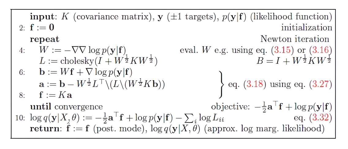
Fig.1. Algoritmo 3.1 para busca da moda f_hat e LML
- O processo começa com o cálculo da matriz de covariância do kernel K. Como aproximação inicial de f, usa-se o resultado mu_f_train da iteração anterior de otimização dos hiperparâmetros para obter uma convergência mais rápida e estável da iteração anterior de otimização dos hiperparâmetros, em vez de começar a cada vez com um vetor nulo.
- Usando o método de Newton, f_hat é atualizado iterativamente.
- Cálculo da NLML: após a convergência da moda f (quando a variação de LML fica menor que m_tolerance), passamos o valor de NLML ao otimizador.
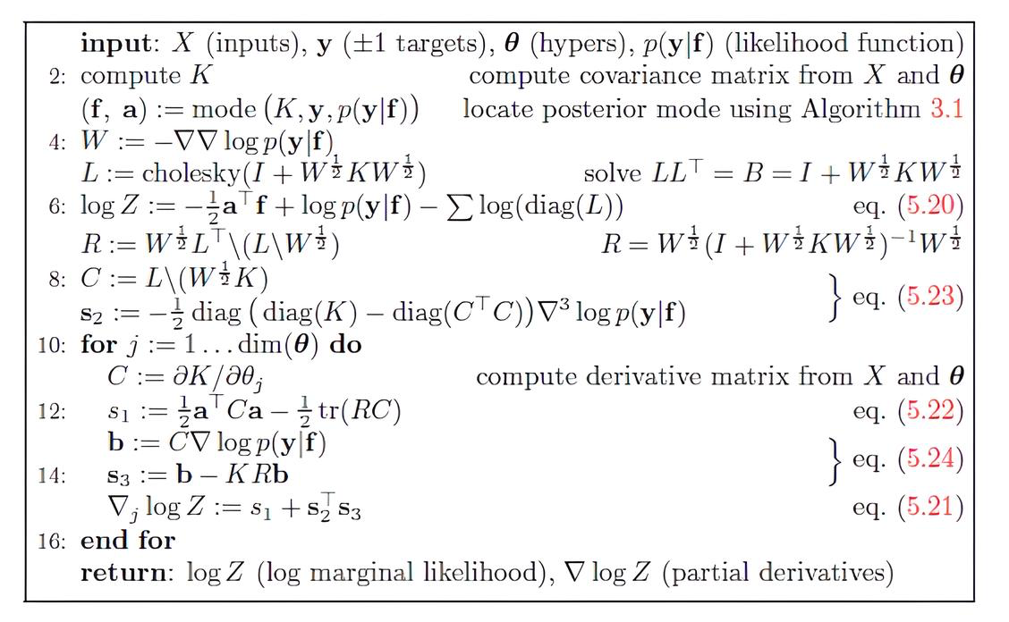
Fig.2. Algoritmo 5.1 para cálculo dos gradientes de LML
- Os gradientes em relação aos hiperparâmetros do kernel incluem o cálculo das matrizes auxiliares R e C. A matriz R é calculada usando cho_solve, e a matriz C, usando LinearEquationsSolutionTriangular.
- Calcula-se a matriz de covariância a posteriori da função latente para os dados de treinamento Σf_train = K−C^TC.
- O gradiente em relação a cada hiperparâmetro do kernel (dK_dtheta_j) é a soma da parte explícita (s1) e das partes implícitas (s2, s3). O cálculo de s1é otimizado com DiagonalTrace, e s3 também usa cho_solve para resolver sistemas.
- Os gradientes em relação aos hiperparâmetros da verossimilhança são calculados com o uso das derivadas da log-verossimilhança e de sua Hessiana em relação aos hiperparâmetros correspondentes. Para isso, são usados os métodos LogLikelihoodGradientParam e LogLikelihoodHessianDerivative do objeto likelihood.
Agora que temos todos os componentes básicos (kernels, verossimilhanças, métodos de inferência), podemos demonstrar como a biblioteca funciona.
Teste da biblioteca com dados sintéticos
O script Gpsynthetic.mq5 nos ajudará a testar nossa biblioteca com dados sintéticos simples. Isso permitirá verificar se os métodos implementados funcionam e se estão corretos.
// --- Include the GP library ---
#include <GP/GP.mqh>

enum IntervalType
  {
   INTERVAL_F = 0, // Confidence interval of the f* latent function
   INTERVAL_Y = 1  // Confidence interval of y* observations
  };

enum Type_inference
  {
   Exact = 0,   // Exact Inference
   Laplace = 1  // Laplace Inference
  };

enum Type_Data
  {
   Regression = 0,    // Regression
   Classification = 1 // Classification
  };

//--- Input parameters
input IntervalType    interval_type  = INTERVAL_F;    // Interval type to display
input Type_Data       DataType       = Classification;
input Type_inference  inf            = Laplace ;        // Inference type

//+------------------------------------------------------------------+
//| Script program start function                                    |
//+------------------------------------------------------------------+
void OnStart()
  {
   string InpFileName1;
   string InpFileName2;
   string InpFileName3;
   string InpFileName4;

   if(DataType == Regression)
     {
      // Regression data
      InpFileName1 = "Data_Regression/X_train.csv";
      InpFileName2 = "Data_Regression/Y_train.csv";
      InpFileName3 = "Data_Regression/X_test.csv";
      InpFileName4 = "Data_Regression/Y_test.csv";
     }
   else
     {
      InpFileName1 = "Data_Classification/X.csv";  // 200
      InpFileName2 = "Data_Classification/y.csv";
      InpFileName3 = "Data_Classification/X_star.csv";
      InpFileName4 = "Data_Classification/y_star.csv";
     }

//----------- Dataset
   matrix x_train, y_train, x_test, y_test;
   CSVtoMatrix(InpFileName1,x_train);
   CSVtoMatrix(InpFileName2,y_train);
   CSVtoMatrix(InpFileName3,x_test);
   CSVtoMatrix(InpFileName4,y_test);

// Create label vectors from matrices
   vector y_train_ = y_train.Col(0);
   vector y_test_ = y_test.Col(0);

//--- 1. Create kernel objects
   IKernel* rbf = new RBFKernel(1,1);
// IKernel* linear = new LinearKernel(1.0);
// IKernel* periodic = new PeriodicKernel(1.0, 1.0, 5.8);

//--- 2. Combination of kernels (creation of a compound kernel)
// IKernel* functional_kernels_array[] = {rbf, linear, periodic};
// SumKernel* combined_functional_kernel = new SumKernel(functional_kernels_array);

//--- 3. Creating a likelihood object
   ILikelihood* likelihood = NULL; // Declare a pointer of the base type

   if(DataType == Regression)
     {
      likelihood = new GaussianLikelihood(1); // Assign the object
     }

   if(DataType == Classification)
     {
      likelihood = new LogitLikelihood();
     }

//--- 4. Create the inference object
   IInference* inference; // Declare a pointer to the interface
// Select the inference type:
   if(inf == Exact)
     {
      inference = new ExactInference();
     }
   else
     {
      inference = new LaplaceInference(100, 1e-10);
     }

//--- 5. Create an instance of the Gaussian Process model
   CREATE_GP_MODEL(gp_model, rbf, likelihood, inference,x_train, y_train_);
//  CREATE_GP_MODEL(gp_model, combined_functional_kernel, likelihood, inference,x_train, y_train_);
//--------------------------------------------------

   ulong start_time_fit = GetMicrosecondCount();
//--- 6. Hyperparameter optimization
   gp_model.Fit();
   ulong end_time_fit = GetMicrosecondCount();
   double elapsed_time_ms = (end_time_fit - start_time_fit) / 1000.0;
   Print(inference.GetName());
   Print("Fit execution time: ", StringFormat("%.3f", elapsed_time_ms), " ms");
   gp_model.PrintOptimizedKernelParameters();

//--- 7. Forecast for test points
   GPPredictionResult gp_predictions; // create a structure where the prediction results are to be set
   ulong start_time_predict = GetMicrosecondCount();
   gp_model.Predict(x_test, gp_predictions,PROBIT); // MONTE_CARLO,NUM_INTEGR,PROBIT
   ulong end_time_predict = GetMicrosecondCount();
   elapsed_time_ms = (end_time_predict - start_time_predict) / 1000.0;
   Print("Predict execution time: ", StringFormat("%.3f", elapsed_time_ms), " ms");

// --- 8. Classification results
   if(DataType == Classification)
     {
      DisplayClassificationResults(gp_predictions, y_test_);
     }
//--- 9. Regression Results
   if(DataType == Regression)
     {
      VisualizeGP(x_train, y_train, x_test, y_test_, gp_predictions, gp_model, 15);
     }

//--- 10. Releasing memory
   delete gp_model;
  }
Dependendo do DataType selecionado (regressão ou classificação), o script define os caminhos para os arquivos CSV com os dados de treinamento e teste. Pressupõe-se que esses arquivos estejam nas pastas Data_Regression ou Data_Classification, na seção Files.
Em seguida, são criados os objetos dos kernels. Para construir uma função de covariância mais complexa, podem ser usados kernels combinados, como SumKernel ou ProductKernel.
Depois, é criado o objeto da função de verossimilhança (ILikelihood) de acordo com o DataType selecionado, bem como o objeto de inferência (IInference).
Com a macro CREATE_GP_MODEL (ou um construtor semelhante), é criado o modelo de PG, que associa o kernel selecionado, a função de verossimilhança e o método de inferência aos dados de treinamento.
O método gp_model.Fit(int maxiter = 20) inicia o treinamento do modelo. O método agora inclui um novo parâmetro, maxiter, que define o número máximo de iterações.
Após a conclusão do treinamento, o método gp_model.Predict() é usado para gerar previsões em novos dados de teste x_test. Os resultados das previsões (valores médios, covariâncias, probabilidades/rótulos) são salvos na estrutura GPPredictionResult.
Para classificação, é possível selecionar o modo de previsão (PROBIT, NUM_INTEGR, MONTE_CARLO).
Em seguida, o script exibe os resultados da previsão:
- para classificação: é chamada a função DisplayClassificationResults(), que calcula a métrica de acurácia e as probabilidades previstas;
- para regressão: a função VisualizeGP() plota os resultados.
Para regressão, são usados dados sintéticos gerados pela função y = sin(x) + 0.5 * x + noise(sigma = 0.1). Não vamos nos aprofundar nessa tarefa, pois já a analisamos no artigo dedicado à regressão. Apenas observe como o tempo de treinamento melhorou depois que passamos a usar gradientes analíticos e métodos da biblioteca OpenBLAS.
Para classificação binária, são usados dados que representam a tarefa XOR (OU exclusivo). Essa é uma tarefa clássica em machine learning, que demonstra a limitação dos modelos lineares e a necessidade de recorrer a abordagens não lineares, como os PG.
Vamos lembrar que XOR é uma operação lógica que recebe duas entradas binárias (0 ou 1) e retorna 1 se exatamente uma das entradas for igual a 1 e 0 caso contrário. Tabela de verdade XOR:
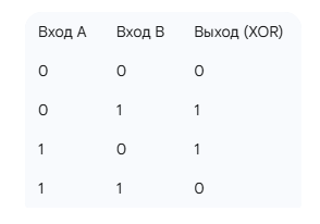
A tarefa de classificação binária XOR consiste em construir um modelo que, com base em duas entradas (A, B), prevê a saída XOR correspondente (0 ou 1). Mas, como nosso modelo trabalha apenas com os rótulos "+1" e "-1", substituiremos o rótulo "0" por "-1".
Os dados para a tarefa XOR são gerados da seguinte forma. São criados pontos de entrada bidimensionais X (X=[x1,x2]), distribuídos aleatoriamente em certo intervalo (por exemplo, [−4,4] em cada eixo). Os rótulos y desses pontos são definidos com base na lógica XOR:
- Se x1 e x2 tiverem o mesmo sinal (ambos positivos ou ambos negativos), então o produto x1⋅x2 será positivo. Nesse caso, o rótulo atribuído será +1.
- Se x1 e x2 tiverem sinais diferentes (um positivo e o outro negativo), então o produto x1⋅x2 será negativo. Nesse caso, o rótulo atribuído será −1.
Assim, os pontos (+,+) e (−,−) pertencem à classe +1, enquanto os pontos (+,−) e (−,+) pertencem à classe −1. Para esta tarefa, usaremos apenas o kernel RBF, pois ele lida muito bem com dependências não lineares, permitindo que os processos gaussianos separem essas classes com eficiência.
Durante os testes, usei 200 observações para treinamento e 100 novos pontos para verificar a acurácia. A acurácia da previsão foi de 98%, o que demonstra a alta eficiência dos PG ao resolver problemas de classificação não linear.
Indicador GPRegressor: Regressão em função do tempo com PG
O indicador é um exemplo de previsão dinâmica de séries temporais financeiras que considera a incerteza. Usando uma janela deslizante para montar a amostra de treinamento e com retreinamento contínuo do modelo, ele implementa o princípio de adaptação às condições de mercado em constante mudança.
//+------------------------------------------------------------------+
//|                                                  GPRegressor.mq5 |
//|                                                           Eugene |
//|                                             https://www.mql5.com |
//+------------------------------------------------------------------+
#property copyright "Eugene"
#property link      "https://www.mql5.com"
#property version   "1.00"
// --- Include the GP library ---
#include <GP/GP.mqh>

#property indicator_chart_window
#property indicator_buffers 3
#property indicator_plots   2

// plot Predicted mean
#property indicator_label1  "Predicted mean"
#property indicator_type1   DRAW_LINE
#property indicator_color1  clrBlue
#property indicator_style1  STYLE_SOLID
#property indicator_width1  2

//--- plot Confidence interval
#property indicator_label2  "Confidence interval"
#property indicator_type2   DRAW_FILLING
#property indicator_color2   clrLightGray
#property indicator_width2  1

//--- Input parameters
input int    WindowLength   = 10;    // Window length for training the model
input int    calculate_bars = 100;   // History depth for calculation
input double zscore         = 1.96;  // z value for the interval (1.96 = 95%)
input bool   ShowRMSE       = false; // Show RMSE metric

//--- Buffers variables for rendering
double  ExtPredictionBuffer[]; // Buffer for predicted values
double  ExtUpperBandBuffer[];  // Buffer for the upper border of the confidence interval
double  ExtLowerBandBuffer[];  // Buffer for the lower border

//--- Global objects
GaussianProcess* g_gp_model       = NULL;
IKernel*         g_kernel         = NULL;
ILikelihood*     g_likelihood     = NULL;
IInference*      g_inference      = NULL;

//--- Global matrix for X_train temporary indices
matrix g_X_train;
//--- Global variables for RMSE data accumulation
vector gp_pred;
vector naive_pred;
vector y_true;
// Flag indicating whether the RMSE has already been calculated (for a one-time calculation)
bool rmse_calculated = false;
string comment;
double gp_rmse,naive_rmse;
//+------------------------------------------------------------------+
//| Custom indicator initialization function                         |
//+------------------------------------------------------------------+
int OnInit()
  {
   if(Bars(Symbol(), Period()) < WindowLength + calculate_bars)
     {
      PrintFormat("Error: Not enough bars to calculate. Minimum %d required. Available: %d",
                  WindowLength + calculate_bars, Bars(Symbol(), Period()));
      return(INIT_FAILED);
     }

   rmse_calculated = false; // Reset the flag on initialization/reinitialization
//--- Initialize global vectors for RMSE
   gp_pred.Resize(calculate_bars-1);
   naive_pred.Resize(calculate_bars-1);
   y_true.Resize(calculate_bars-1);

//--- indicator buffers mapping
   SetIndexBuffer(0, ExtPredictionBuffer, INDICATOR_DATA);
   SetIndexBuffer(1, ExtUpperBandBuffer,  INDICATOR_DATA);
   SetIndexBuffer(2, ExtLowerBandBuffer,  INDICATOR_DATA);

//--- Create kernel, likelihood, and inference method objects
   g_kernel = new RBFKernel(1.0, 1.0);
   if(g_kernel == NULL)
     {
      Print("Failed to create RBFKernel object");
      return(INIT_FAILED);
     }

   g_likelihood = new GaussianLikelihood(0.1);
   if(g_likelihood == NULL)
     {
      Print("Failed to create GaussianLikelihood object");
      delete g_kernel;
      return(INIT_FAILED);
     }

   g_inference = new ExactInference();
   if(g_inference == NULL)
     {
      Print("Failed to create ExactInference object");
      delete g_kernel;
      delete g_likelihood;
      return(INIT_FAILED);
     }

//--- Initialize the feature matrix X_train (one feature - time)
   g_X_train = matrix::Zeros(WindowLength, 1);
   for(int i = 0; i < WindowLength; i++)
     {
      g_X_train[i][0] = (double)(i + 1); // X = [1, 2, ..., WindowLength]
     }

//--- Create the GaussianProcess object
// Pass g_X_train and empty y_train
   vector initial_y_train = vector::Zeros(WindowLength);
   g_gp_model = new GaussianProcess(g_kernel, g_likelihood, g_inference, g_X_train, initial_y_train);
   if(g_gp_model == NULL)
     {
      Print("Failed to create GaussianProcess object");
      delete g_kernel;
      delete g_likelihood;
      delete g_inference;
      return(INIT_FAILED);
     }
   return(INIT_SUCCEEDED);
  }

//+------------------------------------------------------------------+
//|                                                                  |
//+------------------------------------------------------------------+
int OnCalculate(const int32_t rates_total,
                const int32_t prev_calculated,
                const datetime &time[],
                const double &open[],
                const double &high[],
                const double &low[],
                const double &close[],
                const long &tick_volume[],
                const long &volume[],
                const int32_t &spread[])
  {
// Check for sufficient number of bars
   if(rates_total < WindowLength)
     {
      Print("Error: Not enough bars to calculate. At least ", WindowLength, " is required, available: ", rates_total);
      return(0);
     }

   int start;
   if(prev_calculated == 0)
     {
      // Determine where to start the calculation.
      // calculate_bars - history depth to calculate.
      // MathMax(WindowLength, ...) ensures that we start no sooner than there is a full window of data.
      start = MathMax(WindowLength, rates_total - calculate_bars);
      // Initialize all buffers with EMPTY_VALUE
      ArrayInitialize(ExtPredictionBuffer, EMPTY_VALUE);
      ArrayInitialize(ExtUpperBandBuffer,  EMPTY_VALUE);
      ArrayInitialize(ExtLowerBandBuffer,  EMPTY_VALUE);
      // Set the start of rendering buffers
      PlotIndexSetInteger(0, PLOT_DRAW_BEGIN, start);
      PlotIndexSetInteger(1, PLOT_DRAW_BEGIN, start);
      PlotIndexSetInteger(2, PLOT_DRAW_BEGIN, start);
     }
   else
     {
      if(time[rates_total - 1] == time[prev_calculated - 1])
        {
         // This means that a new bar has NOT appeared.
         // We are on the same bar, just new ticks have arrived.
         return(rates_total);
        }
      // If the time of the last bar has changed, then a new closed bar has appeared.
      // Start calculation from prev_calculated to handle all new bars.
      start = prev_calculated;
     }

   for(int i = start; i < rates_total && !IsStopped(); i++)
     {
      // Check if there are enough bars to form a window
      if(i < WindowLength)
        {
         Print("Error: Not enough bars to form a window on bar ", i, ". Required: ", WindowLength, ", available: ", i);
         ExtPredictionBuffer[i] = EMPTY_VALUE;
         ExtUpperBandBuffer[i]  = EMPTY_VALUE;
         ExtLowerBandBuffer[i]  = EMPTY_VALUE;
         continue; // Skip this bar
        }

      // Form y vector from close[i-1], close[i-2], ..., close[i-WindowLength]
      // close[i-1]               - the newest bar in the window
      // close[i-WindowLength] - the oldest bar in the window
      vector y(WindowLength);
      for(int j = 0; j < WindowLength; j++)
        {
         y[WindowLength - 1 - j] = close[i - 1 - j];
        }
      //Print(" y = ", y[WindowLength-1]); // The newest bar in the window

      //--- Data standardization
      double mu_raw = y.Mean();
      // Print("mu_raw = ", mu_raw);
      double sigma_raw = y.Std();
      // Print("sigma_raw = ", sigma_raw);
      vector y_standardized = (y - mu_raw) / sigma_raw;

      //---  Set up training data
      g_gp_model.SetTrainingData(g_X_train, y_standardized);

      //--- Reset initial hyperparameters before Fit()
      vector initial_params(3);
      initial_params[0] = 1.0; // sigma_f (RBFKernel)
      initial_params[1] = 1.0; // length_scale (RBFKernel)
      initial_params[2] = 0.1; // sigma_n (GaussianLikelihood)
      g_gp_model.SetHyperparameters(initial_params);
      // vector params =  g_gp_model.GetCurrentHyperparameters();
      // Print(params);

      // ulong start_time_fit = GetMicrosecondCount();
      //--- Train the model
      if(!g_gp_model.Fit())
        {
         Print("Error: Failed to optimize GP hyperparameters for bar ", i);
         ExtPredictionBuffer[i] = EMPTY_VALUE;
         ExtUpperBandBuffer[i]  = EMPTY_VALUE;
         ExtLowerBandBuffer[i]  = EMPTY_VALUE;
         continue; // Skip the current bar
        }
      //ulong end_time_fit = GetMicrosecondCount();
      // double elapsed_time_ms = (end_time_fit - start_time_fit) / 1000.0;
      //Print("Fit execution time: ", StringFormat("%.3f", elapsed_time_ms), " мс");

      vector params =  g_gp_model.GetCurrentHyperparameters();
      double sigma_f      = params[0]; // sigma_f (RBFKernel)
      double length_scale = params[1]; // length_scale (RBFKernel)
      double sigma_n      = params[2]; // sigma_n (GaussianLikelihood)


      // --- Create a point for forecasting (X_star)
      // Predict the value for the next step after WindowLength
      matrix X_star = matrix::Zeros(1, 1);
      X_star[0][0] = (double)(WindowLength + 1);

      // --- Perform the prediction
      GPPredictionResult gp_predictions;
      if(!g_gp_model.Predict(X_star, gp_predictions))
        {
         Print("Error: Failed to get forecast from GP model for bar ", i);
         ExtPredictionBuffer[i] = EMPTY_VALUE;
         ExtUpperBandBuffer[i]  = EMPTY_VALUE;
         ExtLowerBandBuffer[i]  = EMPTY_VALUE;
         continue;
        }

      // ---
      double predicted_mean_st = gp_predictions.mu_f_star[0];
      // --- Perform the inverse transformation of the predicted mean value
      // back to the original price scale
      double predicted_mean = predicted_mean_st * sigma_raw + mu_raw;

      double sigma_f_star = gp_predictions.Sigma_f_star[0,0]; // dispersion (Σ) of f* signal
      double predicted_variance_st = gp_predictions.Sigma_y_star[0,0]; // dispersion(Σ) of y* observation
      // --- Perform the inverse dispersion transformation
      // The variance is scaled by the square of the standard deviation (sigma_raw) of the data,
      // used for standardization.
      double predicted_variance = predicted_variance_st * sigma_raw * sigma_raw;

      // Calculate the predicted confidence interval
      double std_predict = MathSqrt(predicted_variance);
      double upper_bound = predicted_mean + zscore * std_predict;
      double lower_bound = predicted_mean - zscore * std_predict;

      // --- Save the results to the indicator buffers for rendering
      ExtPredictionBuffer[i] = predicted_mean;
      ExtUpperBandBuffer[i]  = upper_bound;
      ExtLowerBandBuffer[i]  = lower_bound;

      comment = StringFormat("GP Regressor | Mean=%.5f | Upper=%.5f | Lower=%.5f |\n",
                             predicted_mean, upper_bound, lower_bound);
      comment+= StringFormat("Sigma_f = %.5f | Length_Scale = %.5f | Sigma_n = %.5f\n",sigma_f,length_scale,sigma_n);
      comment+= StringFormat("mu f* = %.5f | Σ y* = %.5f | Σ f*= %.5f",predicted_mean_st,predicted_variance_st,sigma_f_star);
      Comment(comment);
      // Debug output
      Print("Bar forecast ", i, ": Mean=", DoubleToString(predicted_mean, Digits()),
            " Upper=", DoubleToString(upper_bound, Digits()),
            " Lower=", DoubleToString(lower_bound, Digits()));
     }

// ---  Calculate RMSE to evaluate the efficiency of the GP forecast model compared to a simple "naive" forecast
   if(ShowRMSE && !rmse_calculated)
     {
      vector returns(calculate_bars-1);
      for(int j=0; j <calculate_bars-1;j++)
        {
         // true value
         y_true[j] = close[rates_total - calculate_bars + j];
         //Print("y_true[j]", y_true[j] );

         // GP forecast:
         gp_pred[j] = ExtPredictionBuffer[rates_total-calculate_bars + j];
         //Print("gp_pred[j]", gp_pred[j] );

         // "Naive" forecast (price tomorrow = price today):
         naive_pred[j] = close[rates_total - calculate_bars + j-1];
         // Print("naive_pred[j]", naive_pred[j] );

         returns[j] = close[rates_total - calculate_bars + j]  - close[rates_total - calculate_bars + j-1];
        }

      gp_rmse=gp_pred.RegressionMetric(y_true,REGRESSION_RMSE);
      naive_rmse=naive_pred.RegressionMetric(y_true,REGRESSION_RMSE);
      double std_returns = returns.Std(); // standard deviation of Close increments
      comment = comment + StringFormat("\nRMSE GP: %.5f | RMSE Naive: %.5f | StdDev Returns Close: %.5f ", gp_rmse, naive_rmse, std_returns);
      rmse_calculated = true;
     }
   Comment(comment);
//--- Return rates_total for the next call
   return(rates_total);
  }
//+------------------------------------------------------------------+
//| Custom indicator deinitialization function                       |
//+------------------------------------------------------------------+
void OnDeinit(const int reason)
  {
//--- Clear the comment on the chart
   Comment("");
//--- Free up the allocated memory for the GP object
   if(g_gp_model != NULL)
     {
      delete g_gp_model;
     }
  }
//+------------------------------------------------------------------+
Parâmetros de entrada:
- WindowLength: comprimento da janela de dados (em barras) para treinar o modelo de PG.
- calculate_bars: profundidade do histórico para cálculo e renderização do indicador.
- zscore: quantidade de desvios padrão para construir o intervalo de confiança (por exemplo, 1.96 para 95%).
- ShowRMSE: flag para exibir a raiz do erro quadrático médio (RMSE) da previsão.
Inicialização (OnInit):
- Objetos globais. São criados e inicializados os objetos globais do kernel (RBFKernel), da função de verossimilhança (GaussianLikelihood) e do método de inferência (ExactInference).
- Atributos X_train. GPRegressor implementa regressão em função do tempo, usando os índices de tempo (de 1 a WindowLength) dentro da janela de treinamento como atributos de entrada X.
- Modelo GaussianProcess. O objeto g_gp_model é inicializado com os componentes especificados, enquanto y_train fica inicialmente vazio e será preenchido dinamicamente.
Laço principal de cálculo (OnCalculate):
- Geração dos dados: em cada barra, são extraídos os últimos WindowLength valores de fechamento para montar o vetor y.
- Padronização dos dados: y é padronizado (transformado para média zero e variância unitária) a fim de aumentar a estabilidade numérica dos cálculos com PG.
- Atualização e treinamento do modelo:
Os hiperparâmetros são redefinidos para os valores iniciais antes de cada treinamento (g_gp_model.SetHyperparameters).
O modelo GP é treinado na janela atual de preços padronizados com g_gp_model.Fit().
- Previsão: para prever a próxima barra, é criado o ponto X_star com o índice de tempo WindowLength + 1. O método g_gp_model.Predict() gera a previsão, retornando a média (mu_f_star) e a variância (Sigma_y_star) para os dados padronizados.
- Despadronização: a média e a variância previstas são transformadas de volta para a escala original de preços usando a média (mu_raw) e o desvio padrão (sigma_raw) da janela atual.
- Intervalo de confiança: os limites superior e inferior do intervalo são calculados com base na média e no desvio padrão transformados, usando o valor zscore definido pelo usuário para o número de desvios padrão.
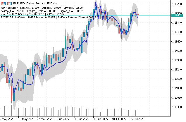
Fig.3. Previsão do modelo regressor e 95% do intervalo de confiança
Cálculo da métrica RMSE:
O indicador exibe uma única vez, a pedido do usuário, as estatísticas de RMSE para as previsões do modelo de PG e da previsão "ingênua" (em que o preço de amanhã = o preço de hoje) para as últimas calculate_bars barras. Essas estatísticas ajudam a avaliar objetivamente a eficiência atual do modelo.
Por exemplo, valores típicos para EURUSD no timeframe de um minuto podem ser: RMSE GP (0.00032) | RMSE Naive (0.00029), enquanto o desvio padrão das variações dos preços de fechamento (StdDev Returns Close) é 0.00029.
O fato de RMSE GP ser maior que RMSE Naive indica desempenho inferior do modelo de PG em comparação com a previsão naive no período analisado. Além disso, a igualdade entre RMSE Naive e StdDev Returns Close é uma característica típica de passeio aleatório, quando as variações futuras de preço não dependem das variações passadas e o valor atual é a melhor previsão.
A partir disso, podemos concluir que, nesse trecho da série temporal, ou não há padrões previsíveis, ou a configuração atual do modelo de PG, que usa apenas o tempo como atributo, ainda não é capaz de extrair informações úteis a ponto de superar a previsão naive.
Indicador GPClassifier: classificação com base em processos gaussianos
O indicador GPClassifier demonstra como criar, treinar e gerar previsões com um modelo de PG em uma tarefa de classificação binária. Como atributos, são usadas as variações dos preços de fechamento, calculadas em uma janela deslizante sobre os dados históricos. A função NormalizeData normaliza a matriz de atributos para estabilizar o treinamento do modelo.
//+------------------------------------------------------------------+
//|                                                 GPClassifier.mq5 |
//|                                                           Eugene |
//|                                             https://www.mql5.com |
//+------------------------------------------------------------------+
#property copyright "Eugene"
#property link       "https://www.mql5.com"
#property version    "1.00"
// --- Include the GP library ---
#include <GP/GP.mqh>

#property indicator_chart_window
#property indicator_buffers 4
#property indicator_plots   2

// plot for predicted class "+1" (up arrows)
#property indicator_label1  "Predicted Class +1"
#property indicator_type1   DRAW_ARROW
#property indicator_color1  clrGreen
#property indicator_width1  1

// plot for predicted class "-1" (down arrows)
#property indicator_label2  "Predicted Class -1"
#property indicator_type2   DRAW_ARROW
#property indicator_color2  clrBlack
#property indicator_width2  1

//--- Input parameters
input int       WindowLength         = 10;    // Window length for training the GP model
input int       NumLags              = 1;     // Number of features
input int       calculate_bars       = 100;   // History depth for calculation
input double    ProbabilityThreshold = 0.5;   // Probability threshold
input int       ArrowShiftPx         = 10;    // Arrow offset in pixels
input bool      ShowACCURACY         = false; // Show accuracy on the chart

//--- Buffers variables for rendering
double  ExtClassUpBuffer[];              // Buffer for displaying UP arrows
double  ExtClassDownBuffer[];            // Buffer for displaying DOWN arrows
double  ExtPredictedClassBuffer[];       // Buffer for storing predicted class labels
double  ExtPredictedProbabilityBuffer[]; // Buffer for storing predicted probabilities

//--- Global Gaussian process objects
GaussianProcess* g_gp_model    = NULL;
IKernel*         g_kernel      = NULL;
ILikelihood*     g_likelihood  = NULL;
IInference*      g_inference   = NULL;

//--- Global variables for classification metrics
bool accuracy_calculated = false;
vector gp_pred,naive_pred,y_true,gp_accuracy,naive_accuracy;
string comment;
int currentsize;
//+------------------------------------------------------------------+
//| Custom indicator initialization function                         |
//+------------------------------------------------------------------+
int OnInit()
  {
   accuracy_calculated = false; // Reset the flag on initialization/reinitialization
//--- Initialize global vectors for Accuracy
   gp_pred.Resize(0);
   naive_pred.Resize(0);
   y_true.Resize(0);
   gp_accuracy.Resize(1);
   naive_accuracy.Resize(1);
   currentsize = 0;
//--- indicator buffers mapping
   SetIndexBuffer(0, ExtClassUpBuffer,     INDICATOR_DATA);    // For up arrows
   SetIndexBuffer(1, ExtClassDownBuffer,   INDICATOR_DATA);    // For down arrows
   SetIndexBuffer(2, ExtPredictedClassBuffer, INDICATOR_CALCULATIONS); //  to store predicted labels
   SetIndexBuffer(3, ExtPredictedProbabilityBuffer, INDICATOR_CALCULATIONS); // to store probabilities
// --- Set arrow symbols
   PlotIndexSetInteger(0, PLOT_ARROW, 225);   // Up arrow for buffer 0
   PlotIndexSetInteger(1, PLOT_ARROW, 226);   // Down arrow for buffer 1
// --- Set the arrow offset in pixels ---
// For the up arrows (buffer 0), use a negative offset so they are above High
   PlotIndexSetInteger(0, PLOT_ARROW_SHIFT, -ArrowShiftPx); // negative = up
// For the down arrows (buffer 1), use a positive offset so they are below Low
   PlotIndexSetInteger(1, PLOT_ARROW_SHIFT, ArrowShiftPx); // positive = down

// Add a check for the ratio of NumLags and WindowLength
   if(NumLags <= 0)
     {
      Print("Error: NumLags must be positive number");
      return(INIT_FAILED);
     }
   if(NumLags >= WindowLength)
     {
      Print("Error: NumLags (", NumLags, ") cannot exceed or be equal to WindowLength (", WindowLength, ").");
      return(INIT_FAILED);
     }

//--- Create kernel, likelihood, and inference method objects
   g_kernel = new RBFKernel(1.0, 1.0);
   if(g_kernel == NULL)
     {
      Print("Failed to create RBFKernel object");
      return(INIT_FAILED);
     }

   g_likelihood = new LogitLikelihood();
   if(g_likelihood == NULL)
     {
      Print("Failed to create LogitLikelihood object");
      delete g_kernel;
      return(INIT_FAILED);
     }

   g_inference = new LaplaceInference();
   if(g_inference == NULL)
     {
      Print("Failed to create ExactInference object");
      delete g_kernel;
      delete g_likelihood;
      return(INIT_FAILED);
     }
// --- Create the GaussianProcess model
// Pass empty matrices for X_train and y_train.
// They will be overridden in OnCalculate.
   g_gp_model = new GaussianProcess(g_kernel, g_likelihood, g_inference,matrix::Zeros(1,1), vector::Zeros(1));
   if(g_gp_model == NULL)
     {
      Print("Failed to create GaussianProcess object");
      delete g_kernel;
      delete g_likelihood;
      delete g_inference;
      return(INIT_FAILED);
     }
   return(INIT_SUCCEEDED);
  }
//+------------------------------------------------------------------+
//| Custom indicator iteration function                              |
//+------------------------------------------------------------------+
int OnCalculate(const int32_t rates_total,
                const int32_t prev_calculated,
                const datetime &time[],
                const double &open[],
                const double &high[],
                const double &low[],
                const double &close[],
                const long &tick_volume[],
                const long &volume[],
                const int32_t &spread[])
  {
// Check for sufficient number of bars
   if(rates_total < WindowLength + NumLags + 1)
     {
      Print("Error: Not enough bars to calculate. Required at least ", WindowLength + NumLags + 1, ", available: ", rates_total);
      return(0);
     }

   int start;
   if(prev_calculated == 0)
     {
      start = MathMax(WindowLength + NumLags + 1, rates_total - calculate_bars);
      // Initialize all EMPTY_VALUE buffers
      ArrayInitialize(ExtClassUpBuffer, EMPTY_VALUE);
      ArrayInitialize(ExtClassDownBuffer, EMPTY_VALUE);
      // Number of initial bars without rendering and values in DataWindow
      PlotIndexSetInteger(0, PLOT_DRAW_BEGIN, start);
      PlotIndexSetInteger(1, PLOT_DRAW_BEGIN, start);
     }
   else
     {
      if(time[rates_total - 1] == time[prev_calculated - 1])
        {
         return(rates_total);
        }
      start = prev_calculated;
     }

// --- Main forecast calculation loop
   for(int i = start; i < rates_total && !IsStopped(); i++)
     {
      // Check if there are enough bars to form X and y window
      if(i < WindowLength + NumLags + 1)
        {
         ExtClassUpBuffer[i] = EMPTY_VALUE;
         ExtClassDownBuffer[i] = EMPTY_VALUE;
         continue;
        }

      // --- Step 1: Generate training data (X_train and y_train)
      matrix X_train = matrix::Zeros(WindowLength, NumLags);
      vector y_train = vector::Zeros(WindowLength);

      for(int j = 0; j < WindowLength; j++)
        {
         // Calculate the bar index in the 'close' array for the current observation in the window.
         int idx = i - WindowLength + j;
         // Formation of features (lags) for the current observation (X_train[j] strings)
         for(int lag_idx = 0; lag_idx < NumLags; lag_idx++)
           {
            // Example:
            // lag_idx = 0: (close[idx - 1] - close[idx - 2]) - increment of the previous bar
            // lag_idx = 1: (close[idx - 2] - close[idx - 3]) - increment of the bar before last
            X_train[j,lag_idx] = close[idx - 1 - lag_idx] - close[idx - 2 - lag_idx];
           }

         // Y_train[j]: Binary label for price increment on idx bar.
         if(close[idx] - close[idx - 1] > 0)
           {
            y_train[j] = 1; // Price increased
           }
         else
           {
            y_train[j] = -1; // Price decreased or remained unchanged
           }

        }
      // Print(y_train);

      // --- Normalize X_train
      matrix X_train_norm;
      vector out_mean;
      vector out_std;
      if(!NormalizeData(X_train,X_train_norm,out_mean,out_std))
        {
         Print("Error: Failed to normalize feature matrix ", i);
         continue;
        }

      // --- Step 2: Feed data into the GP model
      g_gp_model.SetTrainingData(X_train_norm, y_train);

      // Reset initial hyperparameters before each Fit() training
      vector initial_params(2);
      initial_params[0] = 1.0; // sigma_f (RBFKernel)
      initial_params[1] = 1.0; // length_scale (RBFKernel)
      g_gp_model.SetHyperparameters(initial_params);

      // --- Step 3: Train the model
     //  ulong start_time_fit = GetMicrosecondCount();
      if(!g_gp_model.Fit())
        {
         Print("Error: Failed to optimize GP hyperparameters for bar ", i);
         ExtClassUpBuffer[i] = EMPTY_VALUE;
         ExtClassDownBuffer[i] = EMPTY_VALUE;
         continue;
        }
       // ulong end_time_fit = GetMicrosecondCount();
      //  double elapsed_time_ms = (end_time_fit - start_time_fit) / 1000.0;
       // Print("Fit execution time: ", StringFormat("%.3f", elapsed_time_ms), " ms");

      // --- Step 4: Create a point for the X_star forecast
      // X_star - increment of prices of previous NumLags closed bars,
      // used to predict the movement of the current bar (i bar).
      matrix X_star = matrix::Zeros(1, NumLags);
      for(int lag_idx = 0; lag_idx < NumLags; lag_idx++)
        {
         X_star[0][lag_idx] = close[i - 1 - lag_idx] - close[i - 2 - lag_idx];
        }
      //  X_star should also be normalized using the same means and standard deviations,
      //  as for the corresponding X_train columns.
      for(int lag_idx = 0; lag_idx < NumLags; lag_idx++)
        {
         X_star[0][lag_idx] = (X_star[0][lag_idx] - out_mean[lag_idx]) / out_std[lag_idx];
        }

      // --- Step 5: Perform the prediction
      GPPredictionResult gp_predictions;
      if(!g_gp_model.Predict(X_star, gp_predictions))
        {
         Print("Error: Failed to get forecast from GP model for bar ", i);
         ExtClassUpBuffer[i] = EMPTY_VALUE;
         ExtClassDownBuffer[i] = EMPTY_VALUE;
         continue;
        }

      double predicted_probability = gp_predictions.predicted_probabilities[0]; // Probability for a single test point
      int predicted_class = (int)gp_predictions.predicted_labels[0]; // Label (+1 or -1)

      // --- Step 6: Save the results to the indicator buffers for rendering
      ExtClassUpBuffer[i] = EMPTY_VALUE;
      ExtClassDownBuffer[i] = EMPTY_VALUE;
      ExtPredictedClassBuffer[i] = predicted_class;
      ExtPredictedProbabilityBuffer[i] = predicted_probability;

      // Add the probability output and the number of features (lags) as a chart comment
      comment = StringFormat("GP Classifier (Lags: %d) | Probability(UP) = %.10f", NumLags, predicted_probability);
      Comment(comment);

      // If the predicted class is "+1" and the probability is above the given threshold
      if(predicted_class == 1 && predicted_probability > ProbabilityThreshold)
        {
         ExtClassUpBuffer[i] = high[i];
        }
      // If the predicted class is "-1" and the probability is above the given threshold
      else
         if(predicted_class == -1 && (1.0 - predicted_probability) > ProbabilityThreshold)
           {
            ExtClassDownBuffer[i] = low[i];
           }

      Print("Bar forecast ", i, ": Probability(UP)=" + DoubleToString(predicted_probability, 10) +
            ", Predicted Class=" + IntegerToString(predicted_class), " time: ", time[i]);
     }

// --- Calculate classification accuracy for assessing the efficiency of the GP predictive model in comparison
//with a "naive" forecast.
   if(ShowACCURACY  && !accuracy_calculated)
     {
      for(int j=0; j <calculate_bars-1;j++)
        {
         // index to the current bar
         int bar_idx = rates_total - calculate_bars + j;

         if(ExtClassUpBuffer[bar_idx]!= EMPTY_VALUE || ExtClassDownBuffer[bar_idx] != EMPTY_VALUE)
           {
            currentsize = (int)gp_pred.Size();
            currentsize++;
            gp_pred.Resize(currentsize,100);
            naive_pred.Resize(currentsize,100);
            y_true.Resize(currentsize,100);

            // True label: count to the current bar
            if(close[bar_idx] - close[bar_idx - 1] > 0)
              {
               y_true[currentsize-1] = 1; // Price increased
              }
            else
              {
               y_true[currentsize-1] = -1; // Price decreased or remained unchanged
              }
            // Print("y_true",  y_true[currentsize-1] );

            // GP forecast: count to the current bar
            gp_pred[currentsize-1] = ExtPredictedClassBuffer[bar_idx];
            // Print(" gp_pred",  gp_pred[currentsize-1]);

            // "Naive" forecast: the "for tomorrow" bar label is equal to the "today" label
            if(close[bar_idx - 1] - close[bar_idx - 2] > 0)
              {
               naive_pred[currentsize-1] = 1;
              }
            else
              {
               naive_pred[currentsize-1] = -1;
              }
           }

        }

      if(!(int)gp_pred.Size()==0)
        {
         gp_accuracy=gp_pred.ClassificationMetric(y_true,CLASSIFICATION_ACCURACY);
         naive_accuracy=naive_pred.ClassificationMetric(y_true,CLASSIFICATION_ACCURACY);
         comment += StringFormat("\nGP Accuracy: %.2f %% | Naive Accuracy: %.2f %%", gp_accuracy[0], naive_accuracy[0]);
         comment += StringFormat("\nNumber of Filtered Signals: %d", (int)gp_pred.Size());
        }
      else
        {
         comment += StringFormat("\n No Signals for ProbabilityThreshold: %.4f ", ProbabilityThreshold);
        }
      accuracy_calculated = true;
     }
   Comment(comment);
//--- Return rates_total for the next call
   return(rates_total);
  }

//+------------------------------------------------------------------+
//| Custom indicator deinitialization function                       |
//+------------------------------------------------------------------+
void OnDeinit(const int reason)
  {
// Clear the comment on the chart when deleting the indicator
   Comment("");

   if(g_gp_model != NULL)
     {
      delete g_gp_model;
     }
  }
Parâmetros de entrada:
- WindowLength: comprimento da janela de dados para treinar o modelo. Número de observações na amostra de treinamento.
- NumLags: quantidade de lags (variações de preço defasadas). Por exemplo, se NumLags = 1, o atributo será apenas a variação do preço na barra anterior. Se NumLags = 3, os atributos serão as variações do preço nas três barras anteriores, e assim por diante.
- calculate_bars: define o número das últimas barras no gráfico para as quais o indicador será calculado e plotado.
- ProbabilityThreshold: limiar de probabilidade. O indicador exibe sinais com setas para cima ou para baixo se a probabilidade prevista de movimento do preço na direção correspondente exceder esse limiar.
- ArrowShiftPx: deslocamento das setas em pixels em relação à máxima e à mínima da barra.
- ShowACCURACY: flag para exibir as métricas de acurácia da classificação no gráfico.
OnInit(): inicialização do modelo de PG:
- Criamos o kernel RBF, a função de verossimilhança e o método de inferência:
- g_kernel = new RBFKernel(1.0, 1.0)
- g_likelihood = new LogitLikelihood()
- g_inference = new LaplaceInference()
- Criamos o modelo GaussianProcess:
- g_gp_model = new GaussianProcess(g_kernel, g_likelihood, g_inference, matrix::Zeros(1,1), vector::Zeros(1));
- O objeto g_gp_model é criado com estruturas iniciais vazias para os dados de treinamento X_train e y_train. Esses dados serão preenchidos e atualizados dinamicamente a cada barra dentro da função OnCalculate.
OnCalculate(): laço principal de cálculo:
1. Verificação de barras suficientes: antes de iniciar os cálculos, verificamos se há barras suficientes no gráfico para formar a janela de treinamento, considerando WindowLength, NumLags e uma barra para o rótulo a ser previsto.
2. Geração dos dados de treinamento (X_train e y_train):
- Atributos X_train: a cada etapa, a matriz de atributos X_train é montada em uma janela deslizante. Cada linha é uma observação, e as colunas são as variações de preço (lags) nas NumLags barras anteriores.
- Rótulos y_train: rótulos binários que indicam a direção do movimento do preço na próxima barra: "1" (o preço subiu) ou "-1" (o preço caiu ou não se alterou).
3. Normalização de X_train: a matriz de atributos é padronizada para aumentar a estabilidade numérica. Os valores médios (out_mean) e os desvios padrão (out_std) obtidos nessa etapa são salvos para normalizar o ponto de previsão.
4. Atualização e treinamento do modelo de PG:
- g_gp_model.SetTrainingData(X_train_stdard, y_train): os dados de treinamento são atualizados a cada barra.
- g_gp_model.SetHyperparameters(initial_params): os hiperparâmetros do kernel são redefinidos e otimizados novamente para cada nova barra.
- g_gp_model.Fit(): executa o treinamento na janela atual de dados padronizados.
5. Criação e normalização do novo ponto de previsão (X_star): o ponto é normalizado usando os vetores out_mean e out_std.
6. Execução da previsão: o método g_gp_model.Predict(X_star, gp_predictions) retorna a probabilidade prevista de alta (predicted_probabilities[0]) e o rótulo binário (predicted_labels[0]).
7. Desenho e exibição: dependendo de predicted_class e ProbabilityThreshold, uma seta para cima ou para baixo é desenhada no gráfico. As informações sobre a probabilidade da previsão e a classe prevista são exibidas no comentário do gráfico e no log.
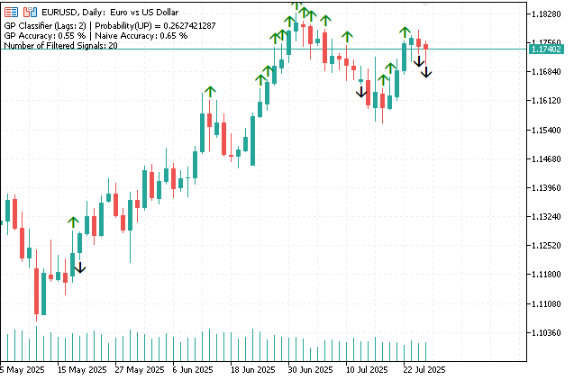
Fig.4. Resultado da previsão do indicador GP Classifier (kernel RBF)
Cálculo das métricas de acurácia (ShowACCURACY)
Quando o parâmetro ShowACCURACY é ativado, o indicador executa um único cálculo da acurácia da classificação para as últimas calculate_bars barras, comparando as previsões do modelo de PG com a previsão "ingênua".
Os rótulos reais (y_true) são definidos como a direção efetiva do movimento do preço. A previsão do modelo de PG (gp_pred) corresponde aos rótulos previstos pelo modelo de PG. A previsão "ingênua" (naive_pred) assume que a direção do próximo movimento do preço será a mesma do movimento anterior, por exemplo, se o preço subiu na barra anterior, a previsão ingênua será de alta.
São comparadas as métricas CLASSIFICATION_ACCURACY de ambos os modelos (gp_accuracy e naive_accuracy), e os resultados são exibidos no comentário do gráfico. Isso permite avaliar objetivamente o desempenho do modelo de PG em relação a um benchmark simples.
Considerações finais
Hoje concluímos a análise do modelo de classificação com processos gaussianos. Depois de examinar em detalhes os fundamentos teóricos, conseguimos criar uma versão básica da biblioteca que permite resolver tanto problemas de regressão quanto de classificação. O teste com dados sintéticos confirmou que os componentes implementados da biblioteca funcionam corretamente, incluindo a aplicação eficiente de gradientes analíticos e da biblioteca de alto desempenho OpenBLAS para estabilidade numérica e velocidade.
Os indicadores GPRegressor e GPClassifier demonstraram as possibilidades práticas de uso dos PG para a previsão dinâmica de séries temporais financeiras em tempo real, e métricas como RMSE (para regressão) e Accuracy (para classificação) permitiram avaliar objetivamente a eficiência do modelo.
Ainda assim, a implementação da biblioteca está longe do ideal. Apesar de todos os esforços empreendidos, sua velocidade de execução é inferior à de soluções consolidadas, como o scikit-learn. Isso se deve em parte ao fato de termos usado o otimizador MinBleic, que não é o mais rápido.
Portanto, as melhorias futuras da biblioteca podem passar por:
- uso de um otimizador baseado em gradientes mais eficiente. Em particular, precisaremos de um algoritmo L-BFGS rápido, que supera significativamente o atual em eficiência para tarefas com grande número de hiperparâmetros;
- implementação mais robusta do método de Newton para a aproximação de Laplace. A adição de busca linear permitirá encontrar a moda da distribuição a posteriori de forma mais eficiente e confiável, melhorando a convergência da otimização resultante;
- implementação de métodos esparsos. Diferentemente da abordagem atual com matrizes completas, o uso de representações esparsas permitirá treinar modelos com volumes de dados significativamente maiores, abrindo novas possibilidades de escalabilidade e aplicação dos PG.
Programas utilizados no artigo
| # | Nome | Tipo | Descrição |
|---|---|---|---|
| 1 | GPClassifier.mq5 | Indicador | Classifica a direção do preço um passo à frente com base em probabilidades previstas (treinamento online) |
| 2 | GPRegressor.mq5 | Indicador | Prevê o preço e o intervalo de confiança um passo à frente (treinamento online) |
| 3 | GPsynthetic.mq5 | Script | Verificação do modelo de processo gaussiano com dados sintéticos |
| 4 | GP.mqh | Biblioteca de classes | Classe GaussianProcess, que combina o kernel, a função de verossimilhança e o método de inferência; classe GPOptimizationObjective, responsável pela otimização |
| 5 | Inference.mqh | Biblioteca de classes | Interface IInference e suas implementações, que definem os métodos de inferência |
| 6 | Kernels.mqh | Biblioteca de classes | Interface IKernel e implementações dos kernels de covariância |
| 7 | Likelihoods.mqh | Biblioteca de classes | Interface ILikelihood e implementações das funções de verossimilhança |
| 8 | StructUtils.mqh | Biblioteca de classes | Funções auxiliares e estruturas de dados |
| 9 | DataRegression | CSV | Dados para o script GPsynthetic.mq5 |
| 10 | DataClassification | CSV | Dados para o script GPsynthetic.mq5 |
Traduzido do russo pela MetaQuotes Ltd.
Artigo original: https://www.mql5.com/ru/articles/19013
Aviso: Todos os direitos sobre esses materiais pertencem à MetaQuotes Ltd. É proibida a reimpressão total ou parcial.
Esse artigo foi escrito por um usuário do site e reflete seu ponto de vista pessoal. A MetaQuotes Ltd. não se responsabiliza pela precisão das informações apresentadas nem pelas possíveis consequências decorrentes do uso das soluções, estratégias ou recomendações descritas.

 Gerenciador de riscos para robôs de trading (Parte I): include para controle de riscos em EAs
 Previsão no trading e modelos Grey
 Redes neurais em trading: decomposição em vez de aumento de escala (SSCNN)
 MetaTrader 5 Global Optimizer: Uma Estrutura Profissional para Otimizar EAs por Grupos, Subgrupos e Critérios de Robustez

- Aplicativos de negociação gratuitos
- 8 000+ sinais para cópia
- Notícias econômicas para análise dos mercados financeiros
Você concorda com a política do site e com os termos de uso
Olá,
Bom dia!
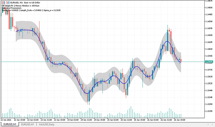
É isso que você quer?
Agora não é exibida a previsão para o próximo passo, mas sim a média e a dispersão na amostra de treinamento.
Muito obrigado, foi muita gentileza sua.
Os modelos de regressão por processos gaussianos podem ser treinados no modo online, permitindo que se adaptem em tempo real à média e à variância dos dados?
Muito obrigado, foi muito gentil da sua parte.
É possível treinar modelos de regressão baseados em processos gaussianos em tempo real, para que eles possam se adaptar à média e à dispersão dos dados em tempo real?