
Gaussian Processes in Machine Learning (Part 2): Implementing and Testing a Classification Model in MQL5

Introduction
In the previous article, we learned about the theoretical foundations of the Bayesian machine learning model — Gaussian Processes — and began creating a GP library in MQL5, describing two key classes: GaussianProcess and GPOptimizationObjective.
Here we will complete the library by taking a detailed look at the implementation of the key interfaces: IKernel, ILikelihood, and IInference. After this, we will test the library on synthetic data and write indicators for classification and regression, demonstrating its operation in online mode — with retraining the model on each new bar.
IKernel interface
The IKernel interface, which you can find in the Kernels.mqh file, is the foundation for implementing covariance kernels in our library. It makes the system flexible and easily extensible: you can add new types of kernels or their combinations without changing the main structure of the code.
interface IKernel { // Calculate the covariance matrix between two data sets virtual matrix Compute(const matrix &X1, const matrix &X2) = 0; // Calculate the derivative of the covariance matrix with respect to the given hyperparameter // param_index: index of the hyperparameter by which the derivative is taken (starting from 0) virtual matrix ComputeDerivative(int param_index) = 0; // Return the current values of all kernel hyperparameters virtual vector GetHyperparameters() const = 0; // Set new values for kernel hyperparameters virtual void SetHyperparameters(const vector ¶ms) = 0; // Return the number of kernel hyperparameters virtual int GetNumHyperparameters() const = 0; // Return the kernel string name virtual string GetName() const = 0; };
The interface defines two of the most important methods that underlie the operation of any kernel:
- Compute(const matrix &X1, const matrix &X2) — compute the K covariance matrix between two data sets.
- ComputeDerivative(int param_index) — compute the derivative of the covariance matrix with respect to one of the kernel hyperparameters. param_index specifies the index of the hyperparameter index with respect to which the derivative is computed.
RBFKernel class (Radial basis kernel)
RBFKernel, also known as the Gaussian or squared exponential kernel, is one of the most commonly used covariance kernels. It is characterized by two hyperparameters: the signal variance σ_f (amplitude) and the length scale l, which determines the function smoothness.
//+------------------------------------------------------------------+ //| Kernel RBF class | //+------------------------------------------------------------------+ class RBFKernel : public IKernel { private: double length; double sigma_f; int n; // Number of rows in X1; int m; // Number of rows in X2; matrix m_K; matrix m_D_sq; // matrix of squared distances ||x_i - x_j||^2 public: //Constructor RBFKernel(double ls, double sf) : length(ls), sigma_f(sf) {} //Destructor ~RBFKernel() {} matrix Compute(const matrix &X1, const matrix &X2) override { n = (int)X1.Rows(); m = (int)X2.Rows(); matrix XX(n, m); if (!XX.GeMM(X1, X2.Transpose(), 1.0, 0.0)) { Print("Error: Failed to calculate XX = X * X^T"); return matrix::Zeros(n, m); } matrix diag1(n, 1); matrix X1_sq = X1 @ X1.Transpose(); diag1.Col(X1_sq.Diag(), 0); matrix diag2(m, 1); matrix X2_sq = X2 @ X2.Transpose(); diag2.Col(X2_sq.Diag(), 0); m_D_sq = matrix::Ones(n, 1) @ diag2.Transpose() + diag1 @ matrix::Ones(1, m) - 2 * XX; m_K = sigma_f * sigma_f * MathExp((-1 * m_D_sq) / (2 * length * length)); return m_K; } matrix ComputeDerivative(int param_index) override { matrix dK(n, m); switch (param_index) { case 0: { dK = (2.0 / sigma_f) * m_K; break; } case 1: { dK = m_K * (m_D_sq / (length * length * length)); break; } } return dK; } vector GetHyperparameters() const override { vector params(2); params[0] = sigma_f; params[1] = length; return params; } void SetHyperparameters(const vector ¶ms) override { if (params.Size() == 2) { sigma_f = params[0]; length = params[1]; } } int GetNumHyperparameters() const override { return 2; } string GetName() const override { return "RBFKernel"; } };
Fortunately, for the RBF kernel, derivatives are easy to find:
-
Derivative with respect to sigma_f:

- Derivative with respect to l:

For the 'length' parameter, we perform element-wise multiplication of the K matrix by (D_sq / length^3), D_sq is the matrix of squared Euclidean distances.
LinearKernel class (Linear kernel)
LinearKernel is a simple covariance kernel that assumes a linear relationship between data points. It is often used when the function is expected to be approximated by a linear model, or as a component in more complex compound kernels.
The linear kernel has one hyperparameter: the σ_l signal variance.
//+------------------------------------------------------------------+ //| Linear kernel class | //+------------------------------------------------------------------+ class LinearKernel : public IKernel { private: double sigma_l; int n; int m; matrix m_K; public: //Constructor LinearKernel(double sl): sigma_l(sl){} //Destructor ~LinearKernel() {} matrix Compute(const matrix &X1, const matrix &X2) override { n = (int)X1.Rows(); m = (int)X2.Rows(); m_K.GeMM(X1, X2.Transpose(), sigma_l * sigma_l, 0.0); return m_K; } matrix ComputeDerivative(int param_index) override { matrix dK(n, m); switch (param_index) { case 0: { // Derivative with respect to sigma_l dK = (2.0 / sigma_l) * m_K; break; } } return dK; } vector GetHyperparameters() const override { vector params(1); params[0] = sigma_l; return params; } void SetHyperparameters(const vector ¶ms) override { if (params.Size() == 1) { sigma_l = params[0]; } } int GetNumHyperparameters() const override { return 1; } string GetName() const override { return "LinearKernel"; } };
ComputeDerivative(int param_index) method:

PeriodicKernel class (Periodic kernel)
PeriodicKernel is used to model data with repeating patterns or seasonality, allowing it to capture cyclical dependencies.
//+------------------------------------------------------------------+ //| Periodic kernel class | //+------------------------------------------------------------------+ class PeriodicKernel : public IKernel { private: double sigma_f; // Signal variance (oscillation amplitude) double length; // Scale length (smoothness of oscillations) double period; // Oscillation period int n; // Number of rows in X1 int m; // Number of rows in X2 matrix m_K; // Covariance matrix matrix m_D; // D matrix (sum of derivatives with respect to d [2 * sin^2(M_PI*distance/period] ) matrix m_distance_dim[]; // Array of difference matrices for each dimension |x_i_k - x_j_k| int m_d_cols; // Number of dimensions (features) (X.Cols()) public: //Constructor PeriodicKernel(double ls, double sf, double p) : sigma_f(sf), length(ls), period(p){} //Destructor ~PeriodicKernel() {} matrix Compute(const matrix &X1, const matrix &X2) override { n = (int)X1.Rows(); m = (int)X2.Rows(); int d = (int)X1.Cols(); m_d_cols = d; m_D = matrix::Zeros(n, m); ArrayResize(m_distance_dim, d); for (int k = 0; k < d; k++) { vector x1_k = X1.Col(k); vector x2_k = X2.Col(k); // Create a matrix where each column is a x1_k vector // (n x 1) * (1 x m) = (n x m) matrix x1_k_copy = x1_k.Outer(vector::Ones(m)) ; // Create a matrix where each row is the transposed vector of x2_k // (n x 1) * (1 x m) = (n x m) matrix x2_k_copy = vector::Ones(n).Outer(x2_k); // Calculate the matrix of all pairwise absolute differences between the elements of vectors x1_k and x2_k matrix distance = MathAbs(x1_k_copy - x2_k_copy); m_distance_dim[k] = distance; // Cache 'distance' for each dimension (feature) matrix sin_term = MathSin(M_PI * distance / period); sin_term = 2.0 * sin_term * sin_term; // 2 * sin^2(u) m_D += sin_term; // Sum up element by element } // Calculate the K matrix m_K = sigma_f * sigma_f * MathExp(-1 * m_D / (length * length)); return m_K; } matrix ComputeDerivative( int param_index) override { matrix dK(n, m); switch (param_index) { case 0: { // Derivative with respect to sigma_f // dK/d(sigma_f) = (2 / sigma_f) * K dK = (2.0 / sigma_f) * m_K; break; } case 1: { // Derivative with respect to 'length' // dK/d(length) = K * (2 * D / length^3) dK = m_K * ( 2.0 * m_D / (length * length * length) ); break; } case 2: { // Derivative with respect to 'period' // dK/d(period) = K * (-1/l^2) * dD/d(period) // dD/d(period) = Sum{k=1:d} (2 * pi * (x_ik - x_jk) / period^2) * sin(2*pi*(x_ik - x_jk)/period) matrix dD_dp = matrix::Zeros(n, m); for (int k = 0; k < m_d_cols; k++) { // Loop through each dimension (column) of the data matrix distance_k = m_distance_dim[k]; // matrix of absolute differences for the k-th dimension matrix u = M_PI * distance_k / period; // Calculate the argument u_k = pi * |x_ik - x_jk| / period matrix sin_2u = MathSin(2.0 * u); // Calculate sin(2 * u_k) // Use the already calculated u to calculate // -pi * |x_ik - x_jk| / period^2 matrix second_term = (-1*u) / period; // Accumulate dD/d(period) for the current measurement dD_dp += 2.0 * sin_2u * second_term; } // unite all parts of the derivative // dK = K * (-1/length^2) * dD_dp dK = m_K * (-1.0 / (length * length)) * dD_dp; break; } } return dK; } vector GetHyperparameters() const override { vector params(3); params[0] = sigma_f; params[1] = length; params[2] = period; return params; } void SetHyperparameters(const vector ¶ms) override { if (params.Size() == 3) { sigma_f = params[0]; length = params[1]; period = params[2]; } } int GetNumHyperparameters() const override { return 3; } string GetName() const override { return "PeriodicKernel"; } };
Derivative of a periodic kernel with respect to the 'period' parameter:
Calculating the derivative with respect to the period parameter is the most difficult, since the 'period' is inside the trigonometric function, which, in turn, is part of the exponential.
The derivative formula is based on the chain rule, where K depends on D, and D depends on 'period' through the sinusoidal terms. The ComputeDerivative implementation iteratively computes the dD_dp component for each dimension, and then computes the final derivative:

Where dD_dp is calculated as the sum of the derivatives 2 * sin^2(M_PI*distance/period) for all dimensions (features).
Composite Kernels
Gaussian processes allow simple covariance kernels to be combined to create more complex models that can describe different aspects of the data (e.g., trend, periodicity, noise). This functionality is implemented through two composite kernels:
- SumKernel — combine multiple kernels by summing their covariance matrices.
- ProductKernel — combine kernels by element-wise multiplication of their covariance matrices.
Both classes manage the hyperparameters of their child kernels, collecting them into a single shared vector for optimization and then distributing them back.
SumKernel class
//+------------------------------------------------------------------+ //| Class for the sum of kernels | //+------------------------------------------------------------------+ class SumKernel : public IKernel { private: IKernel* kernels[]; public: // Constructor SumKernel(IKernel* &input_kernels[]) { ArrayResize(kernels, ArraySize(input_kernels)); ArrayCopy(kernels, input_kernels); } //Destructor ~SumKernel() { for (int i = 0; i < ArraySize(kernels); i++) { if (kernels[i] != NULL) { delete kernels[i]; } } ArrayFree(kernels); } matrix Compute(const matrix &X1, const matrix &X2) override { int n = (int)X1.Rows(); int m = (int)X2.Rows(); matrix sum = matrix::Zeros(n,m); for (int i = 0; i < ArraySize(kernels); i++) { sum += kernels[i].Compute(X1, X2); // Sum the matrices from each child kernel } return sum; } matrix ComputeDerivative(int param_index) override { int current_param_offset = 0; // Start at offset 0 for the first kernel for (int i = 0; i < ArraySize(kernels); i++) { // Get the number of hyperparameters of the current child kernel int num_params_current_kernel = kernels[i].GetNumHyperparameters(); // Check if the global param_index belongs to the current child kernel // param_index should be: // - greater than or equal to the current offset // - strictly less than the current offset + the number of parameters of the current kernel if (param_index >= current_param_offset && param_index < current_param_offset + num_params_current_kernel) { // If param_index belongs to this kernel, calculate its local index int local_param_index = param_index - current_param_offset; // Call ComputeDerivative on the found child kernel and // pass it the local index. // Since the derivative of the sum of kernels with respect to the parameter of one kernel is equal to the derivative // of this particular kernel by this parameter, we can immediately return the result return kernels[i].ComputeDerivative(local_param_index); } // If param_index does not belong to the current kernel, // increase the offset to check the next kernel current_param_offset += num_params_current_kernel; } Print("Error: SumKernel::ComputeDerivative - Parameter index ", param_index, " out of bounds"); return matrix::Zeros(1, 1); } //+---------------------------------------------------------------------------------+ //| The function returns the values of all hyperparameters of the composite kernel | //+---------------------------------------------------------------------------------+ vector GetHyperparameters() const override { vector all_params(GetNumHyperparameters()); int current_idx = 0; for (int i = 0; i < ArraySize(kernels); i++) { // Get the values of the parameters of the current child kernel vector kernel_params = kernels[i].GetHyperparameters(); for (int j = 0; j < (int)kernel_params.Size(); j++) { // Copy the parameters into the common vector all_params[current_idx + j] = kernel_params[j]; } // Update the offset for the next kernel current_idx += (int)kernel_params.Size(); } return all_params; } //+----------------------------------------------------------------------+ //|The function takes a vector of values of all hyperparameters, breaks | //|it into the appropriate parts and assigns them to each child kernel | //+----------------------------------------------------------------------+ void SetHyperparameters(const vector ¶ms) override { int current_idx = 0; for (int i = 0; i < ArraySize(kernels); i++) { // Get the number of hyperparameters of the current child kernel int num_params = kernels[i].GetNumHyperparameters(); vector sub_params(num_params); // Copy the corresponding parameters from the general vector for (int j = 0; j < num_params; j++) { sub_params[j] = params[current_idx + j]; } // Call the SetHyperparameters() method on the current child kernel, // passing it only its own parameters, collected in the sub_params vector kernels[i].SetHyperparameters(sub_params); current_idx += num_params; } } //+--------------------------------------------------------------------------------------+ //| Return the total number of hyperparameters for the entire SumKernel composite kernel | //+--------------------------------------------------------------------------------------+ int GetNumHyperparameters() const override { int total_params = 0; for (int i = 0; i < ArraySize(kernels); i++) { total_params += kernels[i].GetNumHyperparameters(); } return total_params; } string GetName() const override { string name = "Sum("; for (int i = 0; i < ArraySize(kernels); i++) { name += kernels[i].GetName(); if (i < ArraySize(kernels) - 1) name += ","; } name += ")"; return name; } //+------------------------------------------------------------------+ //| Provide external access to the list of child kernels | //+------------------------------------------------------------------+ void GetKernels(IKernel* &output_kernels[]) const { // Copy pointers from the internal kernels array to the passed // output_kernels external array. This provides access to child // kernels in the GaussianProcess::Fit() method, where it is necessary to iterate through // all elementary kernels to set optimization boundaries // of their hyperparameters. ArrayCopy(output_kernels, kernels); } };
- The Compute method computes the final K covariance matrix as the simple sum of the covariance matrices returned by each child kernel. The principle of polymorphism is at work here: even though the kernels array stores pointers of the IKernel* base type, calling kernels[i].Compute(X1, X2) actually calls the specific implementation of Compute for each particular child kernel. This allows SumKernel to work with any kernels inherited from IKernel.
- The key idea behind ComputeDerivative method is that the derivative of the covariance function of the sum of kernels with respect to a specific hyperparameter is equal to the derivative of the covariance function of only the child kernel the given hyperparameter belongs to. This means that ComputeDerivative finds the corresponding child kernel by param_index and returns the derivative exclusively from that kernel. Derivatives with respect to the parameters of other child kernels are considered to be zero.
ProductKernel class
//+------------------------------------------------------------------+ //| Class for the product of kernels | //+------------------------------------------------------------------+ class ProductKernel : public IKernel { private: IKernel* kernels[]; matrix m_X1; matrix m_X2; int n; int m; public: // Constructor: copies pointers to child kernels ProductKernel(IKernel* &input_kernels[]) { ArrayResize(kernels, ArraySize(input_kernels)); ArrayCopy(kernels, input_kernels); } // Destructor ~ProductKernel() { for (int i = 0; i < ArraySize(kernels); i++) { if (kernels[i] != NULL){ delete kernels[i]; } } ArrayFree(kernels); } matrix Compute(const matrix &X1, const matrix &X2) override { n = (int)X1.Rows(); m = (int)X2.Rows(); m_X1 = X1; m_X2 = X2; matrix product = matrix:: Ones(n,m); for (int i = 0; i < ArraySize(kernels); i++) { // Polymorphism: call the Compute() method of each child kernel, // regardless of its specific type, and multiply the result element by element product *= kernels[i].Compute(X1, X2); } return product; } matrix ComputeDerivative(int param_index) override { matrix dK_prod(n, m); // Final derivative matrix int current_param_offset = 0; int target_kernel_idx = -1; // Kernel index the hyperparameter belongs to int local_param_index = -1; // Local index of the hyperparameter in this kernel // Step 1: Find the kernel and local index of the hyperparameter for (int i = 0; i < ArraySize(kernels); i++) { int num_params_current_kernel = kernels[i].GetNumHyperparameters(); if (param_index >= current_param_offset && param_index < current_param_offset + num_params_current_kernel) { target_kernel_idx = i; local_param_index = param_index - current_param_offset; break; } current_param_offset += num_params_current_kernel; } if (target_kernel_idx == -1) { Print("Error: ProductKernel::ComputeDerivative - Parameter index ", param_index, " out of bounds"); return matrix::Zeros(1, 1); } // Step 2: Calculate dK_k / d_theta_j for the target kernel matrix dK_target_kernel = kernels[target_kernel_idx].ComputeDerivative(local_param_index); // Step 3: Calculate the K_m product for all other kernels (m != k) matrix other_kernels_product = matrix::Ones(n, m); for (int i = 0; i < ArraySize(kernels); i++) { if (i != target_kernel_idx) { // Skip the target kernel other_kernels_product = other_kernels_product * kernels[i].Compute(m_X1, m_X2); } } // Step 4: Multiply the results element by element dK_prod = dK_target_kernel * other_kernels_product; return dK_prod; } // Collect the hyperparameter values of all child kernels into a single vector vector GetHyperparameters() const override { vector all_params(GetNumHyperparameters()); int current_idx = 0; for (int i = 0; i < ArraySize(kernels); i++) { vector kernel_params = kernels[i].GetHyperparameters(); for (int j = 0; j < (int)kernel_params.Size(); j++) { all_params[current_idx + j] = kernel_params[j]; } current_idx += (int)kernel_params.Size(); } return all_params; } void SetHyperparameters(const vector ¶ms) override { int current_idx = 0; for (int i = 0; i < ArraySize(kernels); i++) { int num_params_kernel = kernels[i].GetNumHyperparameters(); vector sub_params(num_params_kernel); for (int j = 0; j < num_params_kernel; j++) { sub_params[j] = params[current_idx + j]; } kernels[i].SetHyperparameters(sub_params); current_idx += num_params_kernel; } } int GetNumHyperparameters() const override { int total_params = 0; for (int i = 0; i < ArraySize(kernels); i++) { total_params += kernels[i].GetNumHyperparameters(); } return total_params; } string GetName() const override { string name = "Prod("; for (int i = 0; i < ArraySize(kernels); i++) { name += kernels[i].GetName(); if (i < ArraySize(kernels) - 1) name += "*"; } name += ")"; return name; } //+------------------------------------------------------------------+ //| Provide external access to the list of child kernels | //+------------------------------------------------------------------+ void GetKernels(IKernel* &output_kernels[]) const { ArrayCopy(output_kernels, kernels); } };
- The Compute method computes the final K covariance matrix as the element-wise product of the covariance matrices returned by each child kernel. As in SumKernel, polymorphism is used here to call the Compute method of the corresponding child kernel.
- ComputeDerivative method: To compute the derivative of K with respect to a hyperparameter belonging to a particular K_p child kernel, ProductKernel applies the product rule (Leibniz's rule). The derivative of K with respect to a given parameter is equal to the product of the derivative of the K_p matrix with respect to this parameter and the element-wise product of the covariance matrices of all other child kernels, taken without the derivative:

ILikelihood interface
The ILikelihood interface defines how any likelihood function in our library should work. It allows us to work with different types of data, whether continuous values (as in regression) or discrete categories (as in classification).
//+------------------------------------------------------------------+ //|Interface for likelihood functions | //+------------------------------------------------------------------+ interface ILikelihood { // Compute the p(y|f) log-likelihood for latent values f and observed values y virtual double LogLikelihood(const vector &f, const vector &y) = 0; //----------------------------- Derivatives of the logarithm of the likelihood with respect to f ----------------- // Calculate the vector of the first derivative of the log-likelihood with respect to f (dlp/df) virtual vector LogLikelihoodGradient(const vector &f, const vector &y) = 0; // Compute the second derivative (Hessian) matrix of the log-likelihood with respect to f (d^2lp/df df^T) virtual matrix LogLikelihoodHessian(const vector &f, const vector &y) = 0; // Calculate the vector of the third derivative of the log-likelihood with respect to f (d^3lp/df^3) virtual vector LogLikelihoodThirdDerivative(const vector &f, const vector &y) = 0; //----------------------------- Derivatives of the logarithm of the likelihood with respect to the parameters ----------------- // The first derivative of the log-likelihood with respect to the j-th likelihood hyperparameter. virtual double LogLikelihoodGradientParam(const vector &f, const vector &y, int param_index) = 0; // Hessian derivative of the log-likelihood with respect to the j-th likelihood hyperparameter. virtual matrix LogLikelihoodHessianDerivative(const vector &f, const vector &y, int param_index) = 0; // Return the name of the likelihood function virtual string GetName() const = 0; // Return the current values of the likelihood hyperparameters virtual vector GetHyperparameters() const = 0; // Set new values for the likelihood hyperparameters virtual void SetHyperparameters(const vector ¶ms) = 0; // Return the number of likelihood hyperparameters virtual int GetNumHyperparameters() const = 0; };
GaussianLikelihood class
GaussianLikelihood implements a likelihood function for regression problems assuming normal noise in the observed data.
//+------------------------------------------------------------------+ //| Gaussian likelihood class (for regression problems) | //+------------------------------------------------------------------+ class GaussianLikelihood : public ILikelihood { private: double m_noise_sigma; // Noise parameter (standard deviation) public: // Constructor GaussianLikelihood(double initial_noise_sigma) : m_noise_sigma(initial_noise_sigma) {} // Return the current value of the hyperparameter vector GetHyperparameters() const override { vector params(1); params[0] = m_noise_sigma; return params; } // Set a new hyperparameter value void SetHyperparameters(const vector ¶ms) override { if (params.Size() == 1) { m_noise_sigma = params[0]; } } // Return the number of hyperparameters int GetNumHyperparameters() const override { return 1; } // Calculate the log p(y|f) log-likelihood for a Gaussian distribution double LogLikelihood(const vector &f, const vector &y) override { int n = (int)y.Size(); double noise_variance = m_noise_sigma * m_noise_sigma; vector residual = y - f; // Formula for the logarithm of the density of a multivariate normal distribution return -0.5 / noise_variance * (residual @ residual) - 0.5 * n * MathLog(2 * M_PI * noise_variance); } //------------------ Derivatives with respect to f ----------------------- // Calculate the vector of the first derivative of the log-likelihood with respect to f (dlp/df) vector LogLikelihoodGradient(const vector &f, const vector &y) override { // d(log p(y|f))/df = (y - f) / sigma^2 return (y - f) / (m_noise_sigma * m_noise_sigma); } // Compute the second derivative (Hessian) matrix of the log-likelihood with respect to f (d^2lp/dfdf^T) matrix LogLikelihoodHessian(const vector &f, const vector &y) override { // d^2(log p(y|f))/dfdf^T = -1/sigma^2 * I int n = (int)y.Size(); return matrix::Identity(n, n) * (-1.0 / (m_noise_sigma * m_noise_sigma)); } // Calculate the vector of the third derivative of the log-likelihood with respect to f vector LogLikelihoodThirdDerivative(const vector &f, const vector &y) override { // For Gaussian likelihood d^3(log p(y|f))/df^3 = 0 return vector::Zeros((int)y.Size()); } // ------------------------------ Derivatives with respect to the parameter ----------------------------------- // // Calculate the first derivative of the log-likelihood with respect to the j-th likelihood hyperparameter virtual double LogLikelihoodGradientParam(const vector &f, const vector &y, int param_index) override { // Gaussian likelihood has only 1 hyperparameter: m_noise_sigma (index 0) if (param_index == 0) { // Formula for d(log p(y|f))/d(sigma_n): // = (y-f)^T(y-f) / sigma_n^3 - N / sigma_n vector y_minus_f = y - f; double sn3 = m_noise_sigma * m_noise_sigma * m_noise_sigma; double term1 = (y_minus_f @ y_minus_f) / sn3; double term2 = y.Size() / m_noise_sigma; // N / sigma_n return term1 - term2; } else { return 0.0; } } // Calculate the Hessian derivative of the log-likelihood with respect to the j-th likelihood hyperparameter matrix LogLikelihoodHessianDerivative(const vector &f, const vector &y, int param_index) override { int n = (int)y.Size(); if (param_index == 0) { // Derivative of Hessian with respect to m_noise_sigma: d/d(sigma_n) [-1/sigma_n^2 * I] = (2/sigma_n^3) * I double derivative_coeff = 2.0 / (m_noise_sigma * m_noise_sigma * m_noise_sigma); return matrix::Identity(n, n) * derivative_coeff; } else { return matrix::Zeros(n, n); } } string GetName() const override { return "GaussianLikelihood"; } };
Key methods:
- The GaussianLikelihood constructor initializes a single hyperparameter, the noise standard deviation.
- LogLikelihood() — calculates the p(y∣f) log-likelihood for the probability density function of the multivariate normal distribution:

- LogLikelihoodGradient() — compute the first derivative of the log-likelihood with respect to the latent values of f. This is a vector where each element is equal to:

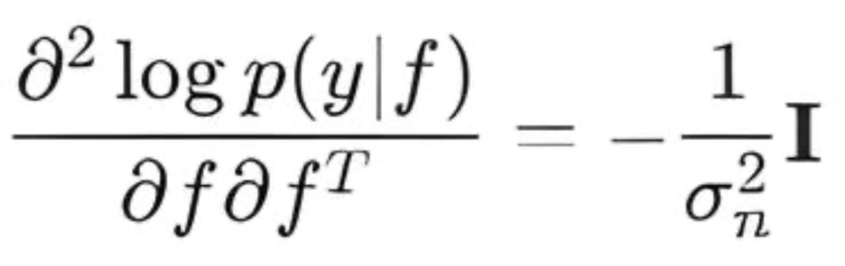
- LogLikelihoodHessian() — calculates the second derivative (Hessian) of the log-likelihood with respect to f. For the Gaussian likelihood, the Hessian is a diagonal matrix:
- LogLikelihoodThirdDerivative() — calculate the third derivative. For Gaussian likelihood, all derivatives above the second are zero.
- LogLikelihoodGradientParam() — calculate the first derivative of the log-likelihood with respect to the m_noise_sigma hyperparameter:

- LogLikelihoodHessianDerivative() — calculate the Hessian derivative of the log-likelihood with respect to the m_noise_sigma hyperparameter:

LogitLikelihood class
LogitLikelihood is used for binary classification, where the observed target values y take the values {−1,+1}. It relates the latent function f to the probability of class membership via a sigmoid function.
The LogitLikelihood implementation provides sigmoid() and Softplus() auxiliary functions with checks for large/small input values.
//+------------------------------------------------------------------+ //| Class for Logit likelihood (y {-1, +1}) | //+------------------------------------------------------------------+ class LogitLikelihood : public ILikelihood { public: // logit_sigmoid(x) = 1 / (1 + exp(-x)) double sigmoid(double x) const { if (x > 100.0) return 1.0; // Avoid NaN occurrences if (x < -100.0) return 0.0; return 1.0 / (1.0 + MathExp(-x)); } // Softplus log(1 + exp(x)) function double Softplus(double x) const { if (x > 100.0) return x; // For very large x, log(1 + exp(x)) ~ x if (x < -100.0) return MathExp(x); // For very small x, log(1 + exp(x)) ~ exp(x) return MathLog(1.0 + MathExp(x)); } public: // Constructor (logit likelihood has no hyperparameters of its own) LogitLikelihood() {} vector GetHyperparameters() const override { return vector::Zeros(0); } void SetHyperparameters(const vector ¶ms) override {} // Return the number of likelihood hyperparameters int GetNumHyperparameters() const override { return 0; } // --- Calculate the log-likelihood: log p(y|f) --- // Formula: sum_i (-log(1 + exp(-y_i * f_i))) double LogLikelihood(const vector &f, const vector &y) override { int n = (int)y.Size(); double total_log_likelihood = 0.0; for (int i = 0; i < n; i++) { total_log_likelihood += -Softplus(-y[i] * f[i]); } return total_log_likelihood; } // Compute the gradient of the log-likelihood with respect to f // Formula: d(log p(y_i|f_i))/df_i = y_i * sigma(-y_i * f_i) vector LogLikelihoodGradient(const vector &f, const vector &y) override { int n = (int)y.Size(); vector grad(n); for (int i = 0; i < n; i++) { grad[i] = y[i] * sigmoid(-y[i] * f[i]); // grad[i] = y[i] * (1 - sigmoid(y[i] * f[i])); equivalent to } return grad; } // Compute the Hessian of the log-likelihood of f (the H diagonal matrix) // Formula: d^2(log p(y_i|f_i))/df_i^2 = -sigma(y_i*f_i)(1 - sigma(y_i*f_i)) matrix LogLikelihoodHessian(const vector &f, const vector &y) override { int n = (int)y.Size(); matrix H = matrix::Identity(n, n); for (int i = 0; i < n; i++) { double sig = sigmoid(y[i] * f[i]); H[i][i] = -1*sig * (1.0 - sig); } return H; } // Calculate the third derivative of the log-likelihood with respect to f // Formula: d^3(log p(y_i|f_i))/df_i^3 = y_i * sigma(-y_i f_i) * (1 - sigma(-y_i f_i)) * (1 - 2*sigma(-y_i f_i)) vector LogLikelihoodThirdDerivative(const vector &f, const vector &y) override { int n = (int)y.Size(); vector third_deriv(n); for (int i = 0; i < n; i++) { double sig_neg_yf = sigmoid(-y[i] * f[i]); third_deriv[i] = y[i] * sig_neg_yf * (1.0 - sig_neg_yf) * (1.0 - 2.0 * sig_neg_yf); // equivalent to // double sig_yf = sigmoid(y[i] * f[i]); // third_deriv[i] = -y[i] * sig_yf * (1.0 - sig_yf) * (1.0 - 2.0 * sig_yf); } return third_deriv; } // LogitLikelihood has no hyperparameters virtual double LogLikelihoodGradientParam(const vector &f, const vector &y, int param_index) override { return 0.0; } // LogitLikelihood has no hyperparameters matrix LogLikelihoodHessianDerivative(const vector &f_latent, const vector &y, int param_index) override { int n = (int)y.Size(); return matrix::Zeros(n, n); } string GetName() const override { return "LogitLikelihood"; } };
Key methods:
- LogLikelihood() — calculate the log-likelihood logp(y∣f). For a binary classification with y {−1,+1}, this is the sum of the logarithms of the binary cross-entropy likelihood:

- LogLikelihoodGradient() — calculate the first derivative of the log-likelihood with respect to f. Each element of the gradient vector is equal to:

- LogLikelihoodHessian() — calculate the second derivative (Hessian) of the log-likelihood with respect to f. For LogitLikelihood, the Hessian is a diagonal matrix where the diagonal elements are equal to:

- LogLikelihoodThirdDerivative() — calculate the third derivative of the log-likelihood with respect to f. Each element of the vector is equal to:

Auxiliary functions and structures
The StructUtils.mqh file contains a set of enumerations, data structures, and functions that make working with GP easier.
    enum PredictMode {
    PROBIT      = 0,  // Probit Approximation
    NUM_INTEGR  = 1,  // Numerical integration
    MONTE_CARLO = 2   // Monte Carlo

};

//--- Structure for prediction results
struct GPPredictionResult
{
    vector mu_f_star;    // Posterior mean for the latent f* function on new data
    matrix Sigma_f_star; // Posterior covariance for the latent f* function on new data

    // Regression-only fields (GaussianLikelihood)
    vector mu_y_star;      // Posterior mean of observations y*
    matrix Sigma_y_star;   // Posterior covariance of observations y*

    // Fields for classification only (LogitLikelihood, ProbitLikelihood, etc.)
    vector predicted_probabilities; // Probabilities p(y*=+1 | X*, D)
    vector predicted_labels;        // Predicted y* labels (+1 or -1)
};

// Structure for the inference result
struct GPInferenceResult {
    double      nlml_value;    // Negative logarithm of the marginal likelihood
    vector      nlml_gradient; // NLML gradient by kernel and likelihood hyperparameters

    // Inference results on training data:
    vector      mu_f_train;    // Posterior mean of the latent function f on the training data
    matrix      Sigma_f_train; // Posterior covariance of the latent function f on the training data (K^−1+W)^−1
    matrix      L_K_noisy;     // Cholesky decomposition K_noisy = cholesky(K + s2n*I)
    matrix      L_B;           // Cholesky decomposition B = I + W^0.5 @ K @ W^0.5
    matrix      sW;            // sW = W^0.5;
    vector      sW_diag;       // sW diagonal
    matrix      sW_K;          // sW @ K
    vector      alpha;         // (K_noisy)^-1 * y
    matrix      H;             // Hessian of the log likelihood d^2 log p(y|f)/df^2 (for LaplaceInference)
    bool        success;       // Flag indicating success of the inference function
};
- The PredictMode enumeration defines different modes for performing predictions in a classification model.
- The GPInferenceResult structure is used to store all key results obtained during the inference.
- The GPPredictionResult structure is designed to store all results obtained after performing a prediction on new (test) data (X_test)
- DiagonalTrace
//+-------------------------------------------------------------------+
//| Compute the trace of the product of two matrices using only       |
//| diagonal elements of the final matrix                             |
//+-------------------------------------------------------------------+
double DiagonalTrace(const matrix &A, const matrix &B)
  {
   ulong m = A.Rows();
   ulong n = A.Cols();
   ulong n_b = B.Rows();
   ulong p = B.Cols();
// Find the minimum size for the diagonal
   ulong k = MathMin(m, p);
   double tr = 0.0;

   for(ulong i = 0; i < k; i++)
     {
      // Dot product of the i-th row of A and the i-th column of B
      tr += A.Row(i)@B.Col(i);
     }
   return tr;
  }
Compute the trace of the product of two matrices A and B (Tr(A @ B)) without having to form the entire product matrix. It does this by summing the scalar products of the rows of matrix A and the corresponding columns of matrix B. This allows to significantly reduce the computational cost compared to full matrix multiplication.
- cho_solve (OpenBLAS LinearEquationsSolutionTriangular wrapper)
 //+-----------------------------------------------------------------------+
   //| Solve the system A*X = B using the Cholesky decomposition A = LL^T  |
   //| Parameters:                                                         |
   //|   c: Lower triangular matrix L from the Cholesky decomposition      |
   //|   b: right side of the system (matrix)                              |
   //| Return: matrix X - system solution                                  |
   //+---------------------------------------------------------------------+
   matrix            cho_solve(const matrix &c, const matrix &b)
     {
    // Check if 'c' matrix is lower triangular one
    if (!c.IsLowerTriangular()) {
        Print("Error: cho_solve - Input matrix 'c' is not lower triangular.");
        return matrix::Zeros(c.Rows(), b.Cols());
    }

// Step 1: Solve L * Y = B
    //  Y -  intermediate matrix, the result of solving L^-1 * B
    matrix Y;
    if (!c.LinearEquationsSolutionTriangular(EQUATIONSFORM_N, b, Y)) {
        PrintFormat("Error: cho_solve- LinearEquationsSolutionTriangular L * Y = B failed. Error Code: %d", GetLastError());
        return matrix::Zeros(c.Rows(), b.Cols());
    }

// Step 2: Solve L^T * X = Y
    //  X - L^T * X = Y system solution, which is equivalent to (L^T)^-1 * Y
    matrix X;
    if (!c.LinearEquationsSolutionTriangular(EQUATIONSFORM_T, Y, X)) {
        PrintFormat("Error: cho_solve- LinearEquationsSolutionTriangular L^T * X = Y failed. Error Code: %d", GetLastError());
        return matrix::Zeros(c.Rows(), b.Cols());
        }
      return X;
     }

   //+------------------------------------------------------------------+
   //| Solve the system Ax = b using the Cholesky decomposition A = LL^T|
   //| Parameters:                                                      |
   //|   c: Lower triangular matrix L from the Cholesky decomposition   |
   //|   b: right side of the system (vector)                           |
   //| Return: vector x - system solution                               |
   //+------------------------------------------------------------------+
   vector            cho_solve(const matrix &c, const vector &b)
     {
      // Check if 'c' matrix is lower triangular one
    if (!c.IsLowerTriangular()) {
        Print("Error: cho_solve - Input matrix 'c' is not lower triangular");
        return vector::Zeros(c.Rows());
    }

    // Step 1: Solve L * y = b
    // y - intermediate vector, the result of solving L^-1 * b
    vector y;
    if (!c.LinearEquationsSolutionTriangular(EQUATIONSFORM_N, b, y)) {
        PrintFormat("Error: cho_solve- LinearEquationsSolutionTriangular L * y = b failed. Error Code: %d", GetLastError());
        return vector::Zeros(c.Rows());
    }

    // Step 2: Solve L^T * x = y
    // x - final solution of the L^T * x = y system, which is equivalent to (L^T)^-1 * y
    vector x;
    if (!c.LinearEquationsSolutionTriangular(EQUATIONSFORM_T, y, x)) {
        PrintFormat("Error: cho_solve- LinearEquationsSolutionTriangular L^T * x = y failed. Error Code: %d", GetLastError());
        return vector::Zeros(c.Rows());
    }
      return x;
     }
The cho_solve function is designed to efficiently solve systems of linear equations Ax=b (or AX=B for matrix B), where the matrix A is obtained from its Cholesky decomposition A=LL^T. Here L is a lower triangular matrix.
Direct computation of A^−1 (A.Inv()) is resource intensive and may be numerically unstable. The Cholesky decomposition, on the other hand, offers a much more efficient and robust approach.
There are two main operations performed inside cho_solve:
- Forward substitution: the system LY=B (or Ly=b) is solved, where L is the input matrix c and Y (or y) is the intermediate result. Since L is a triangular matrix, this solution is relatively fast.
- Backward substitution: then the system L^TX=Y (or L^Tx=y) is solved, where L^T is the transpose of the matrix L. This is also efficient since L^T is an upper triangular matrix.
These operations are implemented using the LinearEquationsSolutionTriangular functions from the OpenBLAS high-performance linear algebra library. This provides significant computational speedups, making them indispensable for resource-intensive machine learning models such as Gaussian processes.
IInference interface
interface IInference
  {
// This method performs inference (i.e., computes the posterior distribution of f)
// and returns the components needed for NLML and prediction
   virtual void Infer(const matrix &X, const vector &y,
                      IKernel *kernel, ILikelihood *likelihood,GPInferenceResult &result) = 0;
   virtual string GetName() const = 0;
  };
The interface allows switching between different inference methods, such as exact inference for Gaussian likelihood and approximate methods for non-Gaussian cases, without changing the core logic of GaussianProcess.
The Infer method is central to this interface. It performs inference of the posterior distribution of the f latent function and returns the components needed for further calculations (NLML and predictions). It accepts the following arguments:
- X — matrix of training features,
- y — vector of training labels,
- kernel — pointer to the Ikernel object,
- likelihood — pointer to the ILikelihood object,
- result — a reference to the GPInferenceResult structure used to store all inference results, including:
- negative logarithm of marginal likelihood (NLML) needed for hyperparameter optimization,
- vector of NLML gradients over all kernel and likelihood hyperparameters,
- auxiliary matrices and vectors: (L_K_noisy, L_B, sW, mu_f_train, Sigma_f_train, alpha) used to calculate NLML gradients and subsequent prediction of new data.
ExactInference class
//+------------------------------------------------------------------+
//| ExactInference For Gaussian likelihood only                      |
//+------------------------------------------------------------------+
class ExactInference : public IInference
  {

public:
                     ExactInference() {}

   void              Infer(const matrix &X, const vector &y,
                           IKernel *kernel, ILikelihood *likelihood,GPInferenceResult &result) override
     {
      if(likelihood.GetName() != "GaussianLikelihood")
        {
         Print("ExactInference supports only GaussianLikelihood");
         result.nlml_value = DBL_MAX;
         return;
        }
      result.success = false;
      int n = (int)y.Size();

      //  Calculate K with current kernel parameters
      matrix K = kernel.Compute(X, X);

      //  Get the noise variance
      vector likelihood_params = likelihood.GetHyperparameters();
      double sigma = likelihood_params[0];
      double variance = sigma * sigma;

      double jitter = 1e-6;
      matrix K_noisy = K + matrix::Identity(n, n) * (variance + jitter);

      if(!K_noisy.Cholesky(result.L_K_noisy))
        {
         PrintFormat("Error: Cholesky decomposition failed. Error Code: %d",GetLastError());
         result.nlml_value = DBL_MAX;
         return;
        }
      //------------- Algorithm 2.1 GPML ---------------------------
      //Calculate alpha (K_noisy^-1 * y) - O(N^2)
      result.alpha = cho_solve(result.L_K_noisy, y);
      //+------------------------------------------------------------------+
      //| NLML = 0.5y^T(K+σ^2*I)^-1*y + 0.5*log|K+σ^2*I| +n/2*Log(2π)      |
      //+------------------------------------------------------------------+
      //+------------------------------------------------------------------+
      //| NLML = 0.5y^T*alpha         + 0.5*log|K+σ^2*I| +n/2*Log(2π)      |
      //+------------------------------------------------------------------+
      // --- Calculate the first term in the NLML equation:
      double data_term = 0.5 * (y @ result.alpha);
      // --- Calculate the second term: 1/2 * log|K + sigma^2*I| = sum(log(L_ii))
      double log_det = MathLog(result.L_K_noisy.Diag()).Sum();
      // --- Calculate the third term: n/2 * log(2π)
      double const_term = 0.5 * n * MathLog(2 * M_PI);
      //--- NLML
      result.nlml_value = data_term + log_det + const_term;

      // -------------------- NLML gradients calculations --------------------------------------
      result.nlml_gradient.Resize(kernel.GetNumHyperparameters() + likelihood.GetNumHyperparameters());
      int current_grad_idx = 0;
      // Calculate (K_noisy^-1)
      matrix K_noisy_inv = cho_solve(result.L_K_noisy, matrix::Identity(n, n));

      // 1. Gradients on kernel hyperparameters
      vector kernel_hyperparams = kernel.GetHyperparameters();
      // Calculate aatK_noisy_inv once before the loop - O(N^2)
      matrix aatK_noisy_inv = result.alpha.Outer(result.alpha) - K_noisy_inv;
      matrix dK_dtheta;
      for(int i = 0; i < (int)kernel_hyperparams.Size(); i++)
        {
         dK_dtheta = kernel.ComputeDerivative(i); // O(N^2)
         result.nlml_gradient[current_grad_idx] = -0.5 * DiagonalTrace(aatK_noisy_inv, dK_dtheta);
         current_grad_idx++;
        }
      // 2. Gradient over noise hyperparameter
      // dNLML/d(sigma^2) = 0.5 * (trace(K_noisy^-1) - alpha^T * alpha )
      double dNLML_d_sigma2n = 0.5 * (K_noisy_inv.Trace() - result.alpha @ result.alpha);
      result.nlml_gradient[current_grad_idx] = dNLML_d_sigma2n * (2.0 * sigma);
      result.success = true;
     }

   string            GetName() const override { return "ExactInference"; }
  };
The ExactInference class is designed to perform exact inference in GP and is only applicable when using Gaussian likelihood. The main focus of its implementation is on the efficient computation of NLML and its analytical gradients. Analytical gradients calculated directly using the equations provide higher accuracy and significantly speed up the optimization process compared to numerical methods.
The inference algorithm consists of several key steps:
- Formation of the Knoisy covariance matrix: First, the K kernel covariance matrix is calculated for the training data. Then the noise variance (variance = sigma * sigma) and a small positive jitter value (1e-6) are added to the diagonal elements of K. This forms the Knoisy matrix;
- Calculation of the αlpha vector;
- Negative log marginal likelihood (NLML) calculation;
- Computing NLML gradients for optimization.
To calculate the required gradients and the NLML itself, the inverse covariance matrix (K+σ2*I)^−1 and the vector α=(K+σ2*I)^−1 * y are required.
The cho_solve function helps calculate these variables as quickly as possible.

LaplaceInference class
LaplaceInference implements Laplace approximation, an approximate inference method applicable to both regression and classification problems in GP.
//+------------------------------------------------------------------+
//| LaplaceInference                                                 |
//+------------------------------------------------------------------+
class LaplaceInference : public IInference
  {
private:
   int               m_max_iterations;
   double            m_tolerance;

public:
                     LaplaceInference(int max_iter = 100, double tolerance = 1e-10) :
                     m_max_iterations(max_iter),
                     m_tolerance(tolerance) {}

   void              Infer(const matrix &X_train, const vector &y,
                           IKernel *kernel, ILikelihood *likelihood, GPInferenceResult &result) override
     {
      result.success = false;
      int n = (int)y.Size();

      //  Calculate K
      matrix K = kernel.Compute(X_train, X_train);
      double jitter = 1e-6;
      K = K + matrix::Identity(n, n) * jitter;

      vector f = (result.mu_f_train.Size() == n) ? result.mu_f_train : vector::Zeros(n);
      bool converged = false;
      matrix W(n, n);                  // W := -Hessian
      matrix L_B(n, n);                // L := cholesky(I + W^0.5*K*W^0.5), B = I + W^0.5*K*W^0.5
      vector b(n);                     // b := Wf + grad loglike p(y|f)
      vector a(n);                     // a := b - W^0.5*L^T\(L\(W^0.5*K*b))
      matrix sW = matrix::Zeros(n, n); // W^0.5
      vector sW_diag(n);               // sqrt(W) vector for storing diagonal elements
      double prev_lml_value = -DBL_MAX; // For the convergence criterion according to LML
      double current_lml_value = -DBL_MAX;
      int iter;
      // --- Step 1: Finding the f_hat mode using Newton's method (According to 3.1 GPML Algorithm) ---
      for(iter = 0; iter < m_max_iterations; iter++)
        {
         // 1. W := - Hessian (diagonal matrix)
         W = -1 * likelihood.LogLikelihoodHessian(f, y);
         // Calculate sW_diag_vector (root of W)
         sW_diag = MathSqrt(W.Diag());
         // 2. L_B := cholesky(I + W^0.5*K*W^0.5)
         // Calculate sW_K = sW * K
         result.sW_K.Resize(n, n);
         for(int i = 0; i < n; i++)
           {
            result.sW_K.Row(sW_diag[i] * K.Row(i),i); // K[i,:] * sW_diag_vector[i]
           }
         // Calculate B = I + sW_K * sW
         matrix temp_sWKsW(n, n);
         for(int j = 0; j < n; j++)
           {
            temp_sWKsW.Col(result.sW_K.Col(j)*sW_diag[j],j) ; // sW_K[:,j] * sW_diag_vector[j]
           }
         matrix B = matrix::Identity(n, n) + temp_sWKsW;
         if(!B.Cholesky(L_B))
           {
            PrintFormat("Error:Cholesky decomposition of B failed. Error Code: %d", GetLastError());
            result.nlml_value = DBL_MAX;
            return;
           }
         result.L_B = L_B; // Save for use in forecasts
         // 3. b := W*f + grad loglike p(y|f)
         b = W.Diag() * f + likelihood.LogLikelihoodGradient(f, y);
         // 4. a := b - W^0.5*L_B^T\(L_B\(W^0.5*K*b))
         a = b - sW_diag*cho_solve(L_B,result.sW_K @ b);
         // 5. f := K * a (new Newton step)
         f = K @ a;

         // --- Calculate the current NLML for the convergence criterion ---
         double log_likelihood_at_f = likelihood.LogLikelihood(f, y);
         double sum_log_diag_L_B = MathLog(L_B.Diag()).Sum();
         current_lml_value = -0.5 * a @ f + log_likelihood_at_f - sum_log_diag_L_B;
         result.nlml_value = -current_lml_value;

         // 6. Convergence check
         double lml_change = current_lml_value - prev_lml_value;
        // PrintFormat("Iter %d: LML = %g, delta LML = %g",iter, current_lml_value, lml_change);

         // Check convergence by LML
         if((lml_change < m_tolerance))
           {
           // PrintFormat("Converged at iter %d: LML = %g, delta LML = %g",iter, current_lml_value, lml_change);
            converged = true;
            break;
           }
         prev_lml_value = current_lml_value;
        }

      if(!converged)
        {
         PrintFormat("Warning: Newton algorithm didn't converge at iteration %d. Final LML: %g (delta: %g, tolerance: %g)",
                     iter, current_lml_value, (current_lml_value - prev_lml_value), m_tolerance);
        }

      //---Save to the GPInferenceResult structure
      result.mu_f_train = f; // Posterior mean of the latent function at training points
      result.H = likelihood.LogLikelihoodHessian(f, y); // Hessian at point f_hat

      // --- Calculating analytical gradients NLML Algorithm 5.1 GPML ---
      result.nlml_gradient.Resize(kernel.GetNumHyperparameters() + likelihood.GetNumHyperparameters());
      int current_grad_idx = 0;
      // ==============================================================================
      // 1. Gradients on KERNEL hyperparameters
      // ==============================================================================
      //   Calculate R := W^0.5*L_B^-T*(L_B^-1*W^0.5)
      result.sW.Diag(sW_diag);
      matrix R(n,n);
      matrix cs = cho_solve(L_B,result.sW);
      for(int i = 0; i < n; i++)
        {
         R.Row(sW_diag[i] * cs.Row(i),i);
        }
      //  Calculate C := L_B^-1 * W^0.5 * K
      // To do this, solve the linear equation: L_B * C = sW * K relative to C
      matrix C;
      if(!L_B.LinearEquationsSolutionTriangular(EQUATIONSFORM_N,result.sW_K, C))
        {
         PrintFormat("Error: LinearEquationsSolutionTriangular L_B * C = W^0.5 * K.Error Code: %d", GetLastError());
         result.nlml_value = DBL_MAX;
         return;
        }
      // Calculate A = Sigma_f_train = (K^−1+W)^−1 = K - C^T @ C
      // Sigma_f_train - posterior covariance matrix of the latent f function on the training data
      matrix CTC = C.Transpose() @ C;
      result.Sigma_f_train = K - CTC;

      //------------------- grad NLML = -(s1 + s2^T*s3)
      // Calculate s2 (first implicit part)
      // s2 := -0.5 * diag( diag(K) - diag(C^T*C) ) * ThirdDerivative loglike by f
      vector third_deriv = likelihood.LogLikelihoodThirdDerivative(f, y);
      //matrix diag;
      //diag.Diag(K.Diag() - CTC.Diag());
      //vector s2 = -0.5 * diag  @ third_deriv;
      vector s2 = -0.5 * (result.Sigma_f_train.Diag() * third_deriv);

      // First, we calculate the gradient of the log-likelihood
      vector log_lik_gradient = likelihood.LogLikelihoodGradient(f, y);
      int num_kernel_hyperparameters = kernel.GetNumHyperparameters();
      for(int j = 0; j < num_kernel_hyperparameters; j++)
        {
         // C2 := dK_dtheta_j (derivative of the kernel matrix with respect to the current hyperparameter)
         matrix dK_dtheta_j = kernel.ComputeDerivative(j);
         ///-------------------------------------------------------------------------------------
         // s1 := 0.5*a^T*C2*a - 0.5 *trace (R*C2) // explicit part of the derivative
         double s1_term1 = 0.5 * (a @(dK_dtheta_j @ a));  // 0.5 * a^T * dK_dtheta_j * a
         // matrix R_dK_dtheta_j = R @ dK_dtheta_j;
         // double s1_term2 = -0.5 * R_dK_dtheta_j.Trace(); // -0.5 * trace(R * dK_dtheta_j)
         double s1_term2 = -0.5 * DiagonalTrace(R,dK_dtheta_j); // more efficient option
         double s1_explicit_part = s1_term1 + s1_term2;
         ///--------------------------------------------------------------------------------------
         // b := C2 * grad loglike
         vector b = dK_dtheta_j @ log_lik_gradient;
         // s3 := b - K * R * b  // second implicit part
         vector s3 = b - K @(R @ b);
         double implicit_part = s2 @ s3; // implicit part of the derivative
         // NLML
         result.nlml_gradient[current_grad_idx] = -(s1_explicit_part + implicit_part);
         current_grad_idx++;
        }
      // ==============================================================================
      // 2. Gradient for LIKELIHOOD hyperparameters dLogLikelihood/d(param_j)
      // ==============================================================================
      if(likelihood.GetNumHyperparameters() > 0)
        {
         vector likelihood_hyperparams = likelihood.GetHyperparameters();

         for(int j = 0; j < (int)likelihood_hyperparams.Size(); j++)
           {
            // Term 1: Derivative of log p(y|f*) with respect to sigma
            double dlogpy_d_param_j = likelihood.LogLikelihoodGradientParam(f, y, j);
            // (the method returns dHessian/d(param_j) = d^3(log p)/d(param_j)d(f)^2)
            matrix dH_param_j = likelihood.LogLikelihoodHessianDerivative(f, y, j);
            // Convert dH_d_param_j to dW_d_param_j (where W = -H)
            matrix dW_d_param_j = -1.0 * dH_param_j;
            double term2_lik = -0.5*DiagonalTrace(result.Sigma_f_train,dW_d_param_j);
            result.nlml_gradient[current_grad_idx] = -(dlogpy_d_param_j + term2_lik);
            current_grad_idx++;
           }
        }
      result.success = true;
     }
   string            GetName() const override { return "LaplaceInference"; }
LaplaceInference(int max_iter = 100, double tolerance = 1e-10) constructor: The class constructor allows initializing the parameters of the iterative Newton method used to find the mode of the posterior distribution.
- max_iter — maximum number of iterations, after which the algorithm will stop, even if convergence is not achieved.
- tolerance — convergence level. The algorithm will stop iterating if the change in the NLML value between successive steps becomes less than this threshold.
The Infer method implements two key algorithms from the book "Gaussian Processes for Machine Learning" (GPML):
- Algorithm 3.1 Finding the posterior distribution mode and calculating NLML,
- Algorithm 5.1 computing NLML gradients from hyperparameters.

Fig. 1. Algorithm 3.1 for searching f_hat and LML modes
- The process begins with the calculation of the K kernel covariance matrix. For faster and more stable convergence, the result of mu_f_train from the previous hyperparameter optimization iteration is used as the initial guess for f, instead of starting from the zero vector each time.
- Using Newton's method, f_hat is iteratively updated.
- Calculating NLML: After the mode f converges (when the change in LML becomes less than m_tolerance), we pass the NLML value to the optimizer.

Fig. 2. Algorithm 5.1 Computing LML gradients
- Gradients over kernel hyperparameters involve the computation of R and C auxiliary matrices. The R matrix is calculated using cho_solve and the C matrix is calculated using LinearEquationsSolutionTriangular.
- The posterior covariance matrix of the latent function is calculated on the training data Σf_train = K−C^TC.
- The gradient for each kernel hyperparameter (dK_dtheta_j) consists of an explicit (s1) and implicit parts (s2, s3). The computation of s1 is optimized by using DiagonalTrace, and s3 also includes cho_solve for solving systems.
- Gradients with respect to the likelihood hyperparameters are calculated using the derivatives of the log-likelihood and its Hessian with respect to the corresponding hyperparameters. For this purpose, the LogLikelihoodGradientParam and LogLikelihoodHessianDerivative methods of the 'likelihood' object are used.
Now that we have all the basic building blocks (kernels, likelihoods, inference methods), let's move on to demonstrating how the library works.
Testing the library on synthetic data
The Gpsynthetic.mq5 script will help us test our library on simple synthetic data. This will allow us to ensure that the implemented methods are working and correct.
// --- Include the GP library ---
#include <GP/GP.mqh>

enum IntervalType
  {
   INTERVAL_F = 0, // Confidence interval of the f* latent function
   INTERVAL_Y = 1  // Confidence interval of y* observations
  };

enum Type_inference
  {
   Exact = 0,   // Exact Inference
   Laplace = 1  // Laplace Inference
  };

enum Type_Data
  {
   Regression = 0,    // Regression
   Classification = 1 // Classification
  };

//--- Input parameters
input IntervalType    interval_type  = INTERVAL_F;    // Interval type to display
input Type_Data       DataType       = Classification;
input Type_inference  inf            = Laplace ;        // Inference type

//+------------------------------------------------------------------+
//| Script program start function                                    |
//+------------------------------------------------------------------+
void OnStart()
  {
   string InpFileName1;
   string InpFileName2;
   string InpFileName3;
   string InpFileName4;

   if(DataType == Regression)
     {
      // Regression data
      InpFileName1 = "Data_Regression/X_train.csv";
      InpFileName2 = "Data_Regression/Y_train.csv";
      InpFileName3 = "Data_Regression/X_test.csv";
      InpFileName4 = "Data_Regression/Y_test.csv";
     }
   else
     {
      InpFileName1 = "Data_Classification/X.csv";  // 200
      InpFileName2 = "Data_Classification/y.csv";
      InpFileName3 = "Data_Classification/X_star.csv";
      InpFileName4 = "Data_Classification/y_star.csv";
     }

//----------- Dataset
   matrix x_train, y_train, x_test, y_test;
   CSVtoMatrix(InpFileName1,x_train);
   CSVtoMatrix(InpFileName2,y_train);
   CSVtoMatrix(InpFileName3,x_test);
   CSVtoMatrix(InpFileName4,y_test);

// Create label vectors from matrices
   vector y_train_ = y_train.Col(0);
   vector y_test_ = y_test.Col(0);

//--- 1. Create kernel objects
   IKernel* rbf = new RBFKernel(1,1);
// IKernel* linear = new LinearKernel(1.0);
// IKernel* periodic = new PeriodicKernel(1.0, 1.0, 5.8);

//--- 2. Combination of kernels (creation of a compound kernel)
// IKernel* functional_kernels_array[] = {rbf, linear, periodic};
// SumKernel* combined_functional_kernel = new SumKernel(functional_kernels_array);

//--- 3. Creating a likelihood object
   ILikelihood* likelihood = NULL; // Declare a pointer of the base type

   if(DataType == Regression)
     {
      likelihood = new GaussianLikelihood(1); // Assign the object
     }

   if(DataType == Classification)
     {
      likelihood = new LogitLikelihood();
     }

//--- 4. Create the inference object
   IInference* inference; // Declare a pointer to the interface
// Select the inference type:
   if(inf == Exact)
     {
      inference = new ExactInference();
     }
   else
     {
      inference = new LaplaceInference(100, 1e-10);
     }

//--- 5. Create an instance of the Gaussian Process model
   CREATE_GP_MODEL(gp_model, rbf, likelihood, inference,x_train, y_train_);
//  CREATE_GP_MODEL(gp_model, combined_functional_kernel, likelihood, inference,x_train, y_train_);
//--------------------------------------------------

   ulong start_time_fit = GetMicrosecondCount();
//--- 6. Hyperparameter optimization
   gp_model.Fit();
   ulong end_time_fit = GetMicrosecondCount();
   double elapsed_time_ms = (end_time_fit - start_time_fit) / 1000.0;
   Print(inference.GetName());
   Print("Fit execution time: ", StringFormat("%.3f", elapsed_time_ms), " ms");
   gp_model.PrintOptimizedKernelParameters();

//--- 7. Forecast for test points
   GPPredictionResult gp_predictions; // create a structure where the prediction results are to be set
   ulong start_time_predict = GetMicrosecondCount();
   gp_model.Predict(x_test, gp_predictions,PROBIT); // MONTE_CARLO,NUM_INTEGR,PROBIT
   ulong end_time_predict = GetMicrosecondCount();
   elapsed_time_ms = (end_time_predict - start_time_predict) / 1000.0;
   Print("Predict execution time: ", StringFormat("%.3f", elapsed_time_ms), " ms");

// --- 8. Classification results
   if(DataType == Classification)
     {
      DisplayClassificationResults(gp_predictions, y_test_);
     }
//--- 9. Regression Results
   if(DataType == Regression)
     {
      VisualizeGP(x_train, y_train, x_test, y_test_, gp_predictions, gp_model, 15);
     }

//--- 10. Releasing memory
   delete gp_model;
  }
Depending on the selected DataType (regression or classification), the script determines the paths to the CSV files with train and test data. These files are assumed to be located in the Data_Regression or Data_Classification folders under Files.
Next, kernel objects are created. To build a more complex covariance function, combined kernels such as SumKernel or ProductKernel can be used.
Then a likelihood function object (ILikelihood) is created depending on the selected DataType, as well as an inference object (IInference).
Using the CREATE_GP_MODEL macro (or a similar constructor), a GP model is created that associates the selected kernel, likelihood function, and inference method with the training data.
The gp_model.Fit(int maxiter = 20) method starts the model training process. The method now has a new parameter responsible for setting the maximum number of 'maxiter' iterations.
After training is complete, the gp_model.Predict() method is used to perform predictions on new (test) data x_test. The prediction results (means, covariances, probabilities/labels) are stored in the GPPredictionResult structure.
For classification, you can select the prediction mode (PROBIT, NUM_INTEGR, MONTE_CARLO).
The script then outputs the prediction results:
- for classification, the DisplayClassificationResults() function is called, which calculates the accuracy metric and predicted probabilities;
- for regression — the VisualizeGP() function is responsible for rendering the results.
For regression, synthetic data generated by the function y = sin(x) + 0.5 * x + noise(sigma = 0.1). We will not dwell on this problem in detail, since we discussed it in the article devoted to regression. Just notice how much the training time has improved since we switched to using analytical gradients and methods from the OpenBLAS library.
For binary classification, data that represents the XOR (exclusive OR) problem is used. This is a classic problem in machine learning that demonstrates the limitations of linear models and the need to use nonlinear approaches, such as GP.
Recall that XOR is a logical operation that takes two binary inputs (0 or 1) and returns 1 if exactly one of the inputs is 1 and 0 otherwise. XOR truth table:

The task of binary XOR classification is to build a model that, given two inputs (A, B), predicts their XOR output (0 and 1). But since our model only works with the +1 and -1 labels, we will replace the 0 label with -1.
The data for the XOR problem is generated as follows. Two-dimensional input points X (X=[x1,x2]) are generated, which are randomly distributed over some range (e.g. [−4,4] on each axis). The y labels for these points are determined based on XOR logic:
- If x1 and x2 have the same signs (both positive or both negative), then their product x1⋅x2 will be positive. In this case, the label is assigned +1.
- If x1 and x2 have different signs (one is positive, the other is negative), then their product x1⋅x2 will be negative. In this case, the label is assigned −1.
Thus, the points (+,+) and (−,−) belong to class +1, and the points (+,−) and (−,+) belong to class −1. For this task, we will use only the RBF kernel, since it copes well with nonlinear dependencies, allowing Gaussian processes to effectively separate such classes.
During the tests, I used 200 observations for training and 100 new points to test the accuracy. The prediction accuracy was 98%, which demonstrates the high efficiency of the GP in solving nonlinear classification problems.
GPRegressor indicator: Regression over time with GP
The indicator is an example of dynamic forecasting of financial time series taking into account uncertainty. By using a sliding window to form the training sample and continuously retraining the model, it implements the principle of adaptation to changing market conditions.
//+------------------------------------------------------------------+
//|                                                  GPRegressor.mq5 |
//|                                                           Eugene |
//|                                             https://www.mql5.com |
//+------------------------------------------------------------------+
#property copyright "Eugene"
#property link      "https://www.mql5.com"
#property version   "1.00"
// --- Include the GP library ---
#include <GP/GP.mqh>

#property indicator_chart_window
#property indicator_buffers 3
#property indicator_plots   2

// plot Predicted mean
#property indicator_label1  "Predicted mean"
#property indicator_type1   DRAW_LINE
#property indicator_color1  clrBlue
#property indicator_style1  STYLE_SOLID
#property indicator_width1  2

//--- plot Confidence interval
#property indicator_label2  "Confidence interval"
#property indicator_type2   DRAW_FILLING
#property indicator_color2   clrLightGray
#property indicator_width2  1

//--- Input parameters
input int    WindowLength   = 10;    // Window length for training the model
input int    calculate_bars = 100;   // History depth for calculation
input double zscore         = 1.96;  // z value for the interval (1.96 = 95%)
input bool   ShowRMSE       = false; // Show RMSE metric

//--- Buffers variables for rendering
double  ExtPredictionBuffer[]; // Buffer for predicted values
double  ExtUpperBandBuffer[];  // Buffer for the upper border of the confidence interval
double  ExtLowerBandBuffer[];  // Buffer for the lower border

//--- Global objects
GaussianProcess* g_gp_model       = NULL;
IKernel*         g_kernel         = NULL;
ILikelihood*     g_likelihood     = NULL;
IInference*      g_inference      = NULL;

//--- Global matrix for X_train temporary indices
matrix g_X_train;
//--- Global variables for RMSE data accumulation
vector gp_pred;
vector naive_pred;
vector y_true;
// Flag indicating whether the RMSE has already been calculated (for a one-time calculation)
bool rmse_calculated = false;
string comment;
double gp_rmse,naive_rmse;
//+------------------------------------------------------------------+
//| Custom indicator initialization function                         |
//+------------------------------------------------------------------+
int OnInit()
  {
   if(Bars(Symbol(), Period()) < WindowLength + calculate_bars)
     {
      PrintFormat("Error: Not enough bars to calculate. Minimum %d required. Available: %d",
                  WindowLength + calculate_bars, Bars(Symbol(), Period()));
      return(INIT_FAILED);
     }

   rmse_calculated = false; // Reset the flag on initialization/reinitialization
//--- Initialize global vectors for RMSE
   gp_pred.Resize(calculate_bars-1);
   naive_pred.Resize(calculate_bars-1);
   y_true.Resize(calculate_bars-1);

//--- indicator buffers mapping
   SetIndexBuffer(0, ExtPredictionBuffer, INDICATOR_DATA);
   SetIndexBuffer(1, ExtUpperBandBuffer,  INDICATOR_DATA);
   SetIndexBuffer(2, ExtLowerBandBuffer,  INDICATOR_DATA);

//--- Create kernel, likelihood, and inference method objects
   g_kernel = new RBFKernel(1.0, 1.0);
   if(g_kernel == NULL)
     {
      Print("Failed to create RBFKernel object");
      return(INIT_FAILED);
     }

   g_likelihood = new GaussianLikelihood(0.1);
   if(g_likelihood == NULL)
     {
      Print("Failed to create GaussianLikelihood object");
      delete g_kernel;
      return(INIT_FAILED);
     }

   g_inference = new ExactInference();
   if(g_inference == NULL)
     {
      Print("Failed to create ExactInference object");
      delete g_kernel;
      delete g_likelihood;
      return(INIT_FAILED);
     }

//--- Initialize the feature matrix X_train (one feature - time)
   g_X_train = matrix::Zeros(WindowLength, 1);
   for(int i = 0; i < WindowLength; i++)
     {
      g_X_train[i][0] = (double)(i + 1); // X = [1, 2, ..., WindowLength]
     }

//--- Create the GaussianProcess object
// Pass g_X_train and empty y_train
   vector initial_y_train = vector::Zeros(WindowLength);
   g_gp_model = new GaussianProcess(g_kernel, g_likelihood, g_inference, g_X_train, initial_y_train);
   if(g_gp_model == NULL)
     {
      Print("Failed to create GaussianProcess object");
      delete g_kernel;
      delete g_likelihood;
      delete g_inference;
      return(INIT_FAILED);
     }
   return(INIT_SUCCEEDED);
  }

//+------------------------------------------------------------------+
//|                                                                  |
//+------------------------------------------------------------------+
int OnCalculate(const int32_t rates_total,
                const int32_t prev_calculated,
                const datetime &time[],
                const double &open[],
                const double &high[],
                const double &low[],
                const double &close[],
                const long &tick_volume[],
                const long &volume[],
                const int32_t &spread[])
  {
// Check for sufficient number of bars
   if(rates_total < WindowLength)
     {
      Print("Error: Not enough bars to calculate. At least ", WindowLength, " is required, available: ", rates_total);
      return(0);
     }

   int start;
   if(prev_calculated == 0)
     {
      // Determine where to start the calculation.
      // calculate_bars - history depth to calculate.
      // MathMax(WindowLength, ...) ensures that we start no sooner than there is a full window of data.
      start = MathMax(WindowLength, rates_total - calculate_bars);
      // Initialize all buffers with EMPTY_VALUE
      ArrayInitialize(ExtPredictionBuffer, EMPTY_VALUE);
      ArrayInitialize(ExtUpperBandBuffer,  EMPTY_VALUE);
      ArrayInitialize(ExtLowerBandBuffer,  EMPTY_VALUE);
      // Set the start of rendering buffers
      PlotIndexSetInteger(0, PLOT_DRAW_BEGIN, start);
      PlotIndexSetInteger(1, PLOT_DRAW_BEGIN, start);
      PlotIndexSetInteger(2, PLOT_DRAW_BEGIN, start);
     }
   else
     {
      if(time[rates_total - 1] == time[prev_calculated - 1])
        {
         // This means that a new bar has NOT appeared.
         // We are on the same bar, just new ticks have arrived.
         return(rates_total);
        }
      // If the time of the last bar has changed, then a new closed bar has appeared.
      // Start calculation from prev_calculated to handle all new bars.
      start = prev_calculated;
     }

   for(int i = start; i < rates_total && !IsStopped(); i++)
     {
      // Check if there are enough bars to form a window
      if(i < WindowLength)
        {
         Print("Error: Not enough bars to form a window on bar ", i, ". Required: ", WindowLength, ", available: ", i);
         ExtPredictionBuffer[i] = EMPTY_VALUE;
         ExtUpperBandBuffer[i]  = EMPTY_VALUE;
         ExtLowerBandBuffer[i]  = EMPTY_VALUE;
         continue; // Skip this bar
        }

      // Form y vector from close[i-1], close[i-2], ..., close[i-WindowLength]
      // close[i-1]               - the newest bar in the window
      // close[i-WindowLength] - the oldest bar in the window
      vector y(WindowLength);
      for(int j = 0; j < WindowLength; j++)
        {
         y[WindowLength - 1 - j] = close[i - 1 - j];
        }
      //Print(" y = ", y[WindowLength-1]); // The newest bar in the window

      //--- Data standardization
      double mu_raw = y.Mean();
      // Print("mu_raw = ", mu_raw);
      double sigma_raw = y.Std();
      // Print("sigma_raw = ", sigma_raw);
      vector y_standardized = (y - mu_raw) / sigma_raw;

      //---  Set up training data
      g_gp_model.SetTrainingData(g_X_train, y_standardized);

      //--- Reset initial hyperparameters before Fit()
      vector initial_params(3);
      initial_params[0] = 1.0; // sigma_f (RBFKernel)
      initial_params[1] = 1.0; // length_scale (RBFKernel)
      initial_params[2] = 0.1; // sigma_n (GaussianLikelihood)
      g_gp_model.SetHyperparameters(initial_params);
      // vector params =  g_gp_model.GetCurrentHyperparameters();
      // Print(params);

      // ulong start_time_fit = GetMicrosecondCount();
      //--- Train the model
      if(!g_gp_model.Fit())
        {
         Print("Error: Failed to optimize GP hyperparameters for bar ", i);
         ExtPredictionBuffer[i] = EMPTY_VALUE;
         ExtUpperBandBuffer[i]  = EMPTY_VALUE;
         ExtLowerBandBuffer[i]  = EMPTY_VALUE;
         continue; // Skip the current bar
        }
      //ulong end_time_fit = GetMicrosecondCount();
      // double elapsed_time_ms = (end_time_fit - start_time_fit) / 1000.0;
      //Print("Fit execution time: ", StringFormat("%.3f", elapsed_time_ms), " мс");

      vector params =  g_gp_model.GetCurrentHyperparameters();
      double sigma_f      = params[0]; // sigma_f (RBFKernel)
      double length_scale = params[1]; // length_scale (RBFKernel)
      double sigma_n      = params[2]; // sigma_n (GaussianLikelihood)


      // --- Create a point for forecasting (X_star)
      // Predict the value for the next step after WindowLength
      matrix X_star = matrix::Zeros(1, 1);
      X_star[0][0] = (double)(WindowLength + 1);

      // --- Perform the prediction
      GPPredictionResult gp_predictions;
      if(!g_gp_model.Predict(X_star, gp_predictions))
        {
         Print("Error: Failed to get forecast from GP model for bar ", i);
         ExtPredictionBuffer[i] = EMPTY_VALUE;
         ExtUpperBandBuffer[i]  = EMPTY_VALUE;
         ExtLowerBandBuffer[i]  = EMPTY_VALUE;
         continue;
        }

      // ---
      double predicted_mean_st = gp_predictions.mu_f_star[0];
      // --- Perform the inverse transformation of the predicted mean value
      // back to the original price scale
      double predicted_mean = predicted_mean_st * sigma_raw + mu_raw;

      double sigma_f_star = gp_predictions.Sigma_f_star[0,0]; // dispersion (Σ) of f* signal
      double predicted_variance_st = gp_predictions.Sigma_y_star[0,0]; // dispersion(Σ) of y* observation
      // --- Perform the inverse dispersion transformation
      // The variance is scaled by the square of the standard deviation (sigma_raw) of the data,
      // used for standardization.
      double predicted_variance = predicted_variance_st * sigma_raw * sigma_raw;

      // Calculate the predicted confidence interval
      double std_predict = MathSqrt(predicted_variance);
      double upper_bound = predicted_mean + zscore * std_predict;
      double lower_bound = predicted_mean - zscore * std_predict;

      // --- Save the results to the indicator buffers for rendering
      ExtPredictionBuffer[i] = predicted_mean;
      ExtUpperBandBuffer[i]  = upper_bound;
      ExtLowerBandBuffer[i]  = lower_bound;

      comment = StringFormat("GP Regressor | Mean=%.5f | Upper=%.5f | Lower=%.5f |\n",
                             predicted_mean, upper_bound, lower_bound);
      comment+= StringFormat("Sigma_f = %.5f | Length_Scale = %.5f | Sigma_n = %.5f\n",sigma_f,length_scale,sigma_n);
      comment+= StringFormat("mu f* = %.5f | Σ y* = %.5f | Σ f*= %.5f",predicted_mean_st,predicted_variance_st,sigma_f_star);
      Comment(comment);
      // Debug output
      Print("Bar forecast ", i, ": Mean=", DoubleToString(predicted_mean, Digits()),
            " Upper=", DoubleToString(upper_bound, Digits()),
            " Lower=", DoubleToString(lower_bound, Digits()));
     }

// ---  Calculate RMSE to evaluate the efficiency of the GP forecast model compared to a simple "naive" forecast
   if(ShowRMSE && !rmse_calculated)
     {
      vector returns(calculate_bars-1);
      for(int j=0; j <calculate_bars-1;j++)
        {
         // true value
         y_true[j] = close[rates_total - calculate_bars + j];
         //Print("y_true[j]", y_true[j] );

         // GP forecast:
         gp_pred[j] = ExtPredictionBuffer[rates_total-calculate_bars + j];
         //Print("gp_pred[j]", gp_pred[j] );

         // "Naive" forecast (price tomorrow = price today):
         naive_pred[j] = close[rates_total - calculate_bars + j-1];
         // Print("naive_pred[j]", naive_pred[j] );

         returns[j] = close[rates_total - calculate_bars + j]  - close[rates_total - calculate_bars + j-1];
        }

      gp_rmse=gp_pred.RegressionMetric(y_true,REGRESSION_RMSE);
      naive_rmse=naive_pred.RegressionMetric(y_true,REGRESSION_RMSE);
      double std_returns = returns.Std(); // standard deviation of Close increments
      comment = comment + StringFormat("\nRMSE GP: %.5f | RMSE Naive: %.5f | StdDev Returns Close: %.5f ", gp_rmse, naive_rmse, std_returns);
      rmse_calculated = true;
     }
   Comment(comment);
//--- Return rates_total for the next call
   return(rates_total);
  }
//+------------------------------------------------------------------+
//| Custom indicator deinitialization function                       |
//+------------------------------------------------------------------+
void OnDeinit(const int reason)
  {
//--- Clear the comment on the chart
   Comment("");
//--- Free up the allocated memory for the GP object
   if(g_gp_model != NULL)
     {
      delete g_gp_model;
     }
  }
//+------------------------------------------------------------------+
Inputs:
- WindowLength — length of the data window (in bars) for training the GP model.
- calculate_bars — history depth for calculating and drawing the indicator.
- zscore — number of standard deviations to construct the confidence interval (e.g. 1.96 for 95%).
- ShowRMSE — flag for displaying the root mean square error (RMSE) of the forecast.
Initialization (OnInit):
- Global objects. Global kernel objects (RBFKernel), likelihood functions (GaussianLikelihood) and inference method (ExactInference) are created and initialized.
- X_train features. GPRegressor implements regression over time using time indices (from 1 to WindowLength) within the training window as X inputs.
- GaussianProcess model. The g_gp_model object is initialized with the specified components, while y_train is initially empty and is to be filled dynamically.
Main calculation loop (OnCalculate):
- Data generation: At each bar, the WindowLength of the latest closing prices is extracted to generate the y vector.
- Data standardization: y is standardized (reduced to zero mean and unit variance) for numerical stability of the GP operation.
- Updating and training the model:
- Hyperparameters are reset to initial values before each training (g_gp_model.SetHyperparameters)
- The GP model is trained on the current window of standardized prices g_gp_model.Fit().
- Prediction: To predict the next bar, X_star point with a time index of WindowLength + 1 is created. The g_gp_model.Predict() method performs prediction, returning the mean (mu_f_star) and variance (Sigma_y_star) for the standardized data.
- Destandardization: The predicted mean and variance are transformed back to the original price scale using the mean (mu_raw) and standard deviation (sigma_raw) of the current window.
- Confidence interval: The upper and lower bounds of the interval are calculated based on the transformed mean and standard deviation using a user-specified zscore standard deviation value.

Fig. 3. Regression model prediction and 95% confidence interval
Calculating the RMSE metric:
The indicator displays RMSE statistics for the GP model forecasts and the "naive" forecast (where tomorrow's price = today's price) for the last calculate_bars once per user request. It helps to objectively evaluate the current model efficiency.
For example, typical indicators for EURUSD on a minute timeframe might be: RMSE GP (0.00032) | RMSE Naive (0.00029), and the standard deviation of closing price increments (StdDev Returns Close) is 0.00029.
The fact that the GP RMSE is higher than the Naive RMSE indicates that the GP model performs worse than the simple naive forecast over the given analyzed period. Moreover, the equality of RMSE Naive and StdDev Returns Close is a characteristic feature of a random walk, where future price changes are independent of past ones, and the current value is the best forecast.
From this, we can conclude that in this section of the time series either there are no predictable patterns, or the current configuration of the GP model (using only time as a feature) is not yet capable of extracting useful information to outperform the naive forecast.
GPClassifier indicator: Classification based on Gaussian processes
The GPClassifier indicator demonstrates the process of creating, training, and predicting a GP model in a binary classification problem. The features used are increments of closing prices, which are calculated in a sliding window of historical data. The NormalizeData function is used to normalize the feature matrix to stabilize the model training.
//+------------------------------------------------------------------+
//|                                                 GPClassifier.mq5 |
//|                                                           Eugene |
//|                                             https://www.mql5.com |
//+------------------------------------------------------------------+
#property copyright "Eugene"
#property link       "https://www.mql5.com"
#property version    "1.00"
// --- Include the GP library ---
#include <GP/GP.mqh>

#property indicator_chart_window
#property indicator_buffers 4
#property indicator_plots   2

// plot for predicted class "+1" (up arrows)
#property indicator_label1  "Predicted Class +1"
#property indicator_type1   DRAW_ARROW
#property indicator_color1  clrGreen
#property indicator_width1  1

// plot for predicted class "-1" (down arrows)
#property indicator_label2  "Predicted Class -1"
#property indicator_type2   DRAW_ARROW
#property indicator_color2  clrBlack
#property indicator_width2  1

//--- Input parameters
input int       WindowLength         = 10;    // Window length for training the GP model
input int       NumLags              = 1;     // Number of features
input int       calculate_bars       = 100;   // History depth for calculation
input double    ProbabilityThreshold = 0.5;   // Probability threshold
input int       ArrowShiftPx         = 10;    // Arrow offset in pixels
input bool      ShowACCURACY         = false; // Show accuracy on the chart

//--- Buffers variables for rendering
double  ExtClassUpBuffer[];              // Buffer for displaying UP arrows
double  ExtClassDownBuffer[];            // Buffer for displaying DOWN arrows
double  ExtPredictedClassBuffer[];       // Buffer for storing predicted class labels
double  ExtPredictedProbabilityBuffer[]; // Buffer for storing predicted probabilities

//--- Global Gaussian process objects
GaussianProcess* g_gp_model    = NULL;
IKernel*         g_kernel      = NULL;
ILikelihood*     g_likelihood  = NULL;
IInference*      g_inference   = NULL;

//--- Global variables for classification metrics
bool accuracy_calculated = false;
vector gp_pred,naive_pred,y_true,gp_accuracy,naive_accuracy;
string comment;
int currentsize;
//+------------------------------------------------------------------+
//| Custom indicator initialization function                         |
//+------------------------------------------------------------------+
int OnInit()
  {
   accuracy_calculated = false; // Reset the flag on initialization/reinitialization
//--- Initialize global vectors for Accuracy
   gp_pred.Resize(0);
   naive_pred.Resize(0);
   y_true.Resize(0);
   gp_accuracy.Resize(1);
   naive_accuracy.Resize(1);
   currentsize = 0;
//--- indicator buffers mapping
   SetIndexBuffer(0, ExtClassUpBuffer,     INDICATOR_DATA);    // For up arrows
   SetIndexBuffer(1, ExtClassDownBuffer,   INDICATOR_DATA);    // For down arrows
   SetIndexBuffer(2, ExtPredictedClassBuffer, INDICATOR_CALCULATIONS); //  to store predicted labels
   SetIndexBuffer(3, ExtPredictedProbabilityBuffer, INDICATOR_CALCULATIONS); // to store probabilities
// --- Set arrow symbols
   PlotIndexSetInteger(0, PLOT_ARROW, 225);   // Up arrow for buffer 0
   PlotIndexSetInteger(1, PLOT_ARROW, 226);   // Down arrow for buffer 1
// --- Set the arrow offset in pixels ---
// For the up arrows (buffer 0), use a negative offset so they are above High
   PlotIndexSetInteger(0, PLOT_ARROW_SHIFT, -ArrowShiftPx); // negative = up
// For the down arrows (buffer 1), use a positive offset so they are below Low
   PlotIndexSetInteger(1, PLOT_ARROW_SHIFT, ArrowShiftPx); // positive = down

// Add a check for the ratio of NumLags and WindowLength
   if(NumLags <= 0)
     {
      Print("Error: NumLags must be positive number");
      return(INIT_FAILED);
     }
   if(NumLags >= WindowLength)
     {
      Print("Error: NumLags (", NumLags, ") cannot exceed or be equal to WindowLength (", WindowLength, ").");
      return(INIT_FAILED);
     }

//--- Create kernel, likelihood, and inference method objects
   g_kernel = new RBFKernel(1.0, 1.0);
   if(g_kernel == NULL)
     {
      Print("Failed to create RBFKernel object");
      return(INIT_FAILED);
     }

   g_likelihood = new LogitLikelihood();
   if(g_likelihood == NULL)
     {
      Print("Failed to create LogitLikelihood object");
      delete g_kernel;
      return(INIT_FAILED);
     }

   g_inference = new LaplaceInference();
   if(g_inference == NULL)
     {
      Print("Failed to create ExactInference object");
      delete g_kernel;
      delete g_likelihood;
      return(INIT_FAILED);
     }
// --- Create the GaussianProcess model
// Pass empty matrices for X_train and y_train.
// They will be overridden in OnCalculate.
   g_gp_model = new GaussianProcess(g_kernel, g_likelihood, g_inference,matrix::Zeros(1,1), vector::Zeros(1));
   if(g_gp_model == NULL)
     {
      Print("Failed to create GaussianProcess object");
      delete g_kernel;
      delete g_likelihood;
      delete g_inference;
      return(INIT_FAILED);
     }
   return(INIT_SUCCEEDED);
  }
//+------------------------------------------------------------------+
//| Custom indicator iteration function                              |
//+------------------------------------------------------------------+
int OnCalculate(const int32_t rates_total,
                const int32_t prev_calculated,
                const datetime &time[],
                const double &open[],
                const double &high[],
                const double &low[],
                const double &close[],
                const long &tick_volume[],
                const long &volume[],
                const int32_t &spread[])
  {
// Check for sufficient number of bars
   if(rates_total < WindowLength + NumLags + 1)
     {
      Print("Error: Not enough bars to calculate. Required at least ", WindowLength + NumLags + 1, ", available: ", rates_total);
      return(0);
     }

   int start;
   if(prev_calculated == 0)
     {
      start = MathMax(WindowLength + NumLags + 1, rates_total - calculate_bars);
      // Initialize all EMPTY_VALUE buffers
      ArrayInitialize(ExtClassUpBuffer, EMPTY_VALUE);
      ArrayInitialize(ExtClassDownBuffer, EMPTY_VALUE);
      // Number of initial bars without rendering and values in DataWindow
      PlotIndexSetInteger(0, PLOT_DRAW_BEGIN, start);
      PlotIndexSetInteger(1, PLOT_DRAW_BEGIN, start);
     }
   else
     {
      if(time[rates_total - 1] == time[prev_calculated - 1])
        {
         return(rates_total);
        }
      start = prev_calculated;
     }

// --- Main forecast calculation loop
   for(int i = start; i < rates_total && !IsStopped(); i++)
     {
      // Check if there are enough bars to form X and y window
      if(i < WindowLength + NumLags + 1)
        {
         ExtClassUpBuffer[i] = EMPTY_VALUE;
         ExtClassDownBuffer[i] = EMPTY_VALUE;
         continue;
        }

      // --- Step 1: Generate training data (X_train and y_train)
      matrix X_train = matrix::Zeros(WindowLength, NumLags);
      vector y_train = vector::Zeros(WindowLength);

      for(int j = 0; j < WindowLength; j++)
        {
         // Calculate the bar index in the 'close' array for the current observation in the window.
         int idx = i - WindowLength + j;
         // Formation of features (lags) for the current observation (X_train[j] strings)
         for(int lag_idx = 0; lag_idx < NumLags; lag_idx++)
           {
            // Example:
            // lag_idx = 0: (close[idx - 1] - close[idx - 2]) - increment of the previous bar
            // lag_idx = 1: (close[idx - 2] - close[idx - 3]) - increment of the bar before last
            X_train[j,lag_idx] = close[idx - 1 - lag_idx] - close[idx - 2 - lag_idx];
           }

         // Y_train[j]: Binary label for price increment on idx bar.
         if(close[idx] - close[idx - 1] > 0)
           {
            y_train[j] = 1; // Price increased
           }
         else
           {
            y_train[j] = -1; // Price decreased or remained unchanged
           }

        }
      // Print(y_train);

      // --- Normalize X_train
      matrix X_train_norm;
      vector out_mean;
      vector out_std;
      if(!NormalizeData(X_train,X_train_norm,out_mean,out_std))
        {
         Print("Error: Failed to normalize feature matrix ", i);
         continue;
        }

      // --- Step 2: Feed data into the GP model
      g_gp_model.SetTrainingData(X_train_norm, y_train);

      // Reset initial hyperparameters before each Fit() training
      vector initial_params(2);
      initial_params[0] = 1.0; // sigma_f (RBFKernel)
      initial_params[1] = 1.0; // length_scale (RBFKernel)
      g_gp_model.SetHyperparameters(initial_params);

      // --- Step 3: Train the model
     //  ulong start_time_fit = GetMicrosecondCount();
      if(!g_gp_model.Fit())
        {
         Print("Error: Failed to optimize GP hyperparameters for bar ", i);
         ExtClassUpBuffer[i] = EMPTY_VALUE;
         ExtClassDownBuffer[i] = EMPTY_VALUE;
         continue;
        }
       // ulong end_time_fit = GetMicrosecondCount();
      //  double elapsed_time_ms = (end_time_fit - start_time_fit) / 1000.0;
       // Print("Fit execution time: ", StringFormat("%.3f", elapsed_time_ms), " ms");

      // --- Step 4: Create a point for the X_star forecast
      // X_star - increment of prices of previous NumLags closed bars,
      // used to predict the movement of the current bar (i bar).
      matrix X_star = matrix::Zeros(1, NumLags);
      for(int lag_idx = 0; lag_idx < NumLags; lag_idx++)
        {
         X_star[0][lag_idx] = close[i - 1 - lag_idx] - close[i - 2 - lag_idx];
        }
      //  X_star should also be normalized using the same means and standard deviations,
      //  as for the corresponding X_train columns.
      for(int lag_idx = 0; lag_idx < NumLags; lag_idx++)
        {
         X_star[0][lag_idx] = (X_star[0][lag_idx] - out_mean[lag_idx]) / out_std[lag_idx];
        }

      // --- Step 5: Perform the prediction
      GPPredictionResult gp_predictions;
      if(!g_gp_model.Predict(X_star, gp_predictions))
        {
         Print("Error: Failed to get forecast from GP model for bar ", i);
         ExtClassUpBuffer[i] = EMPTY_VALUE;
         ExtClassDownBuffer[i] = EMPTY_VALUE;
         continue;
        }

      double predicted_probability = gp_predictions.predicted_probabilities[0]; // Probability for a single test point
      int predicted_class = (int)gp_predictions.predicted_labels[0]; // Label (+1 or -1)

      // --- Step 6: Save the results to the indicator buffers for rendering
      ExtClassUpBuffer[i] = EMPTY_VALUE;
      ExtClassDownBuffer[i] = EMPTY_VALUE;
      ExtPredictedClassBuffer[i] = predicted_class;
      ExtPredictedProbabilityBuffer[i] = predicted_probability;

      // Add the probability output and the number of features (lags) as a chart comment
      comment = StringFormat("GP Classifier (Lags: %d) | Probability(UP) = %.10f", NumLags, predicted_probability);
      Comment(comment);

      // If the predicted class is "+1" and the probability is above the given threshold
      if(predicted_class == 1 && predicted_probability > ProbabilityThreshold)
        {
         ExtClassUpBuffer[i] = high[i];
        }
      // If the predicted class is "-1" and the probability is above the given threshold
      else
         if(predicted_class == -1 && (1.0 - predicted_probability) > ProbabilityThreshold)
           {
            ExtClassDownBuffer[i] = low[i];
           }

      Print("Bar forecast ", i, ": Probability(UP)=" + DoubleToString(predicted_probability, 10) +
            ", Predicted Class=" + IntegerToString(predicted_class), " time: ", time[i]);
     }

// --- Calculate classification accuracy for assessing the efficiency of the GP predictive model in comparison
//with a "naive" forecast.
   if(ShowACCURACY  && !accuracy_calculated)
     {
      for(int j=0; j <calculate_bars-1;j++)
        {
         // index to the current bar
         int bar_idx = rates_total - calculate_bars + j;

         if(ExtClassUpBuffer[bar_idx]!= EMPTY_VALUE || ExtClassDownBuffer[bar_idx] != EMPTY_VALUE)
           {
            currentsize = (int)gp_pred.Size();
            currentsize++;
            gp_pred.Resize(currentsize,100);
            naive_pred.Resize(currentsize,100);
            y_true.Resize(currentsize,100);

            // True label: count to the current bar
            if(close[bar_idx] - close[bar_idx - 1] > 0)
              {
               y_true[currentsize-1] = 1; // Price increased
              }
            else
              {
               y_true[currentsize-1] = -1; // Price decreased or remained unchanged
              }
            // Print("y_true",  y_true[currentsize-1] );

            // GP forecast: count to the current bar
            gp_pred[currentsize-1] = ExtPredictedClassBuffer[bar_idx];
            // Print(" gp_pred",  gp_pred[currentsize-1]);

            // "Naive" forecast: the "for tomorrow" bar label is equal to the "today" label
            if(close[bar_idx - 1] - close[bar_idx - 2] > 0)
              {
               naive_pred[currentsize-1] = 1;
              }
            else
              {
               naive_pred[currentsize-1] = -1;
              }
           }

        }

      if(!(int)gp_pred.Size()==0)
        {
         gp_accuracy=gp_pred.ClassificationMetric(y_true,CLASSIFICATION_ACCURACY);
         naive_accuracy=naive_pred.ClassificationMetric(y_true,CLASSIFICATION_ACCURACY);
         comment += StringFormat("\nGP Accuracy: %.2f %% | Naive Accuracy: %.2f %%", gp_accuracy[0], naive_accuracy[0]);
         comment += StringFormat("\nNumber of Filtered Signals: %d", (int)gp_pred.Size());
        }
      else
        {
         comment += StringFormat("\n No Signals for ProbabilityThreshold: %.4f ", ProbabilityThreshold);
        }
      accuracy_calculated = true;
     }
   Comment(comment);
//--- Return rates_total for the next call
   return(rates_total);
  }

//+------------------------------------------------------------------+
//| Custom indicator deinitialization function                       |
//+------------------------------------------------------------------+
void OnDeinit(const int reason)
  {
// Clear the comment on the chart when deleting the indicator
   Comment("");

   if(g_gp_model != NULL)
     {
      delete g_gp_model;
     }
  }
Inputs:
- WindowLength — length of the data window for training the model. Number of observations in the training sample.
- NumLags — number of lags (price increments). For example, if NumLags = 1, the only feature will be the price increment on the previous bar. If NumLags = 3, the features will be the price increments on the three previous bars, etc.
- calculate_bars — number of the last bars on the chart, for which the indicator will be calculated and drawn.
- ProbabilityThreshold — probability threshold. The indicator displays signals with up/down arrows if the predicted probability of price movement in the corresponding direction exceeds this threshold.
- ArrowShiftPx — offset of the arrows in pixels from the bar extremes.
- ShowACCURACY — flag for displaying classification accuracy metrics on a chart
OnInit() — initialize GP-Model:
- Create an RBF kernel, a likelihood function, and an inference method:
- g_kernel = new RBFKernel(1.0, 1.0)
- g_likelihood = new LogitLikelihood()
- g_inference = new LaplaceInference()
- Create the GaussianProcess model:
- g_gp_model = new GaussianProcess(g_kernel, g_likelihood, g_inference, matrix::Zeros(1,1), vector::Zeros(1));
- The g_gp_model object is created with empty initial matrices for the X_train and y_train training data. This data will be dynamically populated and updated on each bar in the OnCalculate function.
OnCalculate() — main calculation loop:
1. Checking for a sufficient number of bars: Before starting calculations, we make sure that the chart has enough bars to form a training window, taking into account WindowLength, NumLags, and one bar for the predicted label.
2. Formation of training data (X_train and y_train):
- X_train features - at each step, a matrix of X_train features is formed in a sliding window. Each row is an observation, columns are price increments (lags) for the previous NumLags bars.
- y_train labels — binary labels indicating the direction of price movement of the next bar: "1" (price increased) or "-1" (price decreased or remained unchanged).
3. X_train normalization - the feature matrix is standardized for numerical stability. The mean values (out_mean) and standard deviations (out_std) obtained in this step are stored to normalize the prediction point.
4. Updating and training the GP model:
- g_gp_model.SetTrainingData(X_train_stdard, y_train) — training data is updated at each bar.
- g_gp_model.SetHyperparameters(initial_params) — kernel hyperparameters are reset and re-optimized for each new bar
- g_gp_model.Fit() — launch training on the current window of standardized data.
5. Creating and normalizing a new point for prediction (X_star): normalize using the out_mean and out_std vectors.
6. Performing the prediction: the g_gp_model.Predict(X_star, gp_predictions) method returns the predicted probability of an upward move (predicted_probabilities[0]) and the binary label (predicted_labels[0]).
7. Drawing and output: Depending on the predicted_class and ProbabilityThreshold, an up arrow or a down arrow is drawn on the chart. Information about the prediction probability and the predicted class is displayed in the comments on the chart and in the log.

Fig. 4. Prediction result of the GP Classifier indicator (RBF kernel)
Calculating accuracy metrics (ShowACCURACY)
When the ShowACCURACY parameter is enabled, the indicator performs a one-time calculation of the classification accuracy for the last calculate_bars, comparing the GP model forecasts with the "naive" forecast.
True labels (y_true) are defined as the actual direction of price movement. GP Prediction (gp_pred) - the labels predicted by the GP model. The "naive" forecast (naive_pred) assumes that the direction of the next price movement will be the same as the previous movement (for example, if the price rose on the previous bar, the naive forecast is growth).
The CLASSIFICATION_ACCURACY metrics for both models (gp_accuracy and naive_accuracy) are compared and the results are displayed in a chart comment. This allows us to objectively evaluate the performance of the GP model relative to a simple benchmark.
Conclusion
Today we have completed our examination of the Gaussian Process classification model. After a detailed review of the theoretical constructs, we were able to create a basic version of the library that allows us to solve both regression and classification problems. Testing on synthetic data confirmed the proper operation of the implemented library components, including the effective use of analytical gradients and the use of the high-performance OpenBLAS library for numerical stability and speed.
The GPRegressor and GPClassifier indicators demonstrated the practical feasibility of using GP for dynamic forecasting of financial time series in real time, while metrics, such as RMSE (for regression) and Accuracy (for classification), allowed for an objective assessment of the model's performance.
However, the library implementation is far from ideal. Despite all the efforts made, its speed is inferior to well-established solutions, such as scikit-learn. This is partly due to the fact that we were using a relatively slow MinBleic optimizer.
Therefore, further improvement of the library may be related to:
- using a more efficient gradient optimizer. In particular, we need a fast L-BFGS algorithm that significantly outperforms the current one in efficiency for problems with a large number of hyperparameters;
- a more robust implementation of Newton's method for Laplace approximation. Adding a linear search will allow for more efficient and reliable finding of the posterior distribution mode, improving the convergence of the final optimization;
- implementation of sparse methods. Unlike current work with full matrices, using sparse representations will allow the library to train on significantly larger amounts of data, opening up new possibilities for scaling and applying GPs.
Programs used in the article
| # | Name | Type | Description |
|---|---|---|---|
| 1 | GPClassifier.mq5 | Indicator | Classifies one-step-ahead price direction based on predicted probabilities (online training) |
| 2 | GPRegressor.mq5 | Indicator | Predicts price and confidence interval one step ahead (online training) |
| 3 | GPsynthetic.mq5 | Script | Testing the GP model on synthetic data |
| 4 | GP.mqh | Class library | The GaussianProcess class, which combines the kernel, likelihood function, and inference method, and the GPOptimizationObjective class, which is responsible for optimization |
| 5 | Inference.mqh | Class library | The IInference interface and its implementations that define inference methods |
| 6 | Kernels.mqh | Class library | The IKernel interface and implementations of covariance kernels |
| 7 | Likelihoods.mqh | Class library | ILikelihood interface and likelihood function implementations |
| 8 | StructUtils.mqh | Class library | Auxiliary functions and data structures |
| 9 | DataRegression | CSV | GPsynthetic.mq5 script data |
| 10 | DataClassification | CSV | GPsynthetic.mq5 script data |
Translated from Russian by MetaQuotes Ltd.
Original article: https://www.mql5.com/ru/articles/19013
Warning: All rights to these materials are reserved by MetaQuotes Ltd. Copying or reprinting of these materials in whole or in part is prohibited.
This article was written by a user of the site and reflects their personal views. MetaQuotes Ltd is not responsible for the accuracy of the information presented, nor for any consequences resulting from the use of the solutions, strategies or recommendations described.

 Features of Custom Indicators Creation
 Features of Experts Advisors
- Free trading apps
- Over 8,000 signals for copying
- Economic news for exploring financial markets
You agree to website policy and terms of use
Hello,
Good afternoon!

Is this what you wanted?
It now displays the mean and variance of the training sample rather than a one-step-ahead forecast.