Pythonを使用したボラティリティ予測インジケーターの作成

はじめに

しまった！また狩られた…

これは、私が2021年のほぼ毎日の取引を始めるたびに口にしていたフレーズです。チャートと数字に囲まれて、自作の新しい取引システムに胸を膨らませていた矢先、一瞬で口座の半分が消えてしまう…誰かが仮想通貨について一言発しただけで、市場が大荒れしたのです。

おなじみでしょうか。アルゴリズムトレーダーなら誰でも経験しているはずです。履歴データでは完璧に機能するはずのシステムなのに…現実の市場ではどうでしょう。「おや、ボラティリティ、久しぶり！」という感じです。

こんな「冒険」を何度も経験した後、私は怒りに任せて原因を突き止めることにしました。これらの市場のヒステリックな動きを全く予測できないわけはない！私はボラティリティに関する既存の研究を片っ端から調べました。すると面白いことに、解決策は古い手法と最新技術の融合にあることがわかったのです。

この記事では、絶望から実用的なボラティリティ予測システムに至るまでの私の旅路を共有します。退屈な理論や学術用語は一切なし。実際に動く手法と経験談だけをお伝えします。MetaTrader 5とPythonをどう組み合わせたか（最初は相性が悪かった）、機械学習をどう活用したか、途中で遭遇した落とし穴などもお見せします。

この経験で得た最大の教訓は、古典的インジケーターも流行りのニューラルネットも盲信してはいけないということです。複雑なニューラルネットを1週間かけて構築したのに、単純なXGBoostの方が結果が良かったこともありました。あるいは、すべての高度なアルゴリズムが失敗した局面で、単純なボリンジャーバンドが口座を救ったこともあります。

取引はボクシングに似ていて、重要なのは「打撃の強さ」ではなく、「打撃を予測する能力」です。私のシステムは超能力的な予測をおこなうわけではありません。市場のサプライズに備え、取引戦略の安全マージンをタイムリーに確保する手助けをしてくれるだけです。

要するに、アルゴリズムがちょっとしたボラティリティで毎回転んでしまうことに疲れたなら、ようこそ私の世界へ。コード例やチャート、分析を交えて、ありのままにお伝えします。それでは始めましょう。

プロジェクトコンセプト

数か月にわたる実験と市場データの詳細な分析の末、驚くべき精度でボラティリティを予測できるシステムのコンセプトが生まれました。この発見の核心は、ボラティリティは価格と違い、定常性の性質を持つという点です。すなわち、ボラティリティは平均値に回帰し、安定したパターンを形成する傾向があります。この特徴が、ボラティリティの予測を可能かつ実用的なものにしています。

システムは、MetaTrader 5とPythonの強力な組み合わせを基盤としています。それぞれのツールが得意分野を活かします。MetaTrader 5は信頼できる市場データの供給源として機能します。過去の価格データや、最小限の遅延で取得できるリアルタイムデータストリームを提供します。そして、Pythonは分析ラボとして機能します。豊富な機械学習ライブラリ（Sklearn、XGBoost、PyTorch）を活用し、データから有益なパターンを抽出し、ボラティリティの定常性に関する仮説を検証します。

システムのアーキテクチャは、3つの主要レベルで構成されています。

1. データパイプラインはシステムの基盤です。ここでは、MetaTrader 5から取得したデータの一次処理がおこなわれます。具体的には、ノイズの除去、数十種類におよぶボラティリティ指標の計算、そして機械学習モデル用の特徴量の生成です。特に最適化には細心の注意を払っており、システムは遅延やメモリリークなしで動作します。このレイヤーでは、時系列データの定常性テストも実施され、統計的に意味のあるボラティリティパターンが特定されます。
2. 分析コア。この中核部分は、複数の専門化された機械学習モデルからなるアンサンブルで構成されています。それぞれのモデルは異なる時間軸に最適化されており、短期のイントラデイ変動から週単位のトレンドまでをカバーします。テストの結果、特にボラティリティクラスタを検出するタスクにおいては、複雑なニューラルネットワークよりも、シンプルなXGBoostの方が高い予測精度を示すケースが多いことが分かりました。
3. リスクアドバイザー。これはボラティリティ予測に基づいてリスク管理の推奨をおこなうシステムです。将来的にボラティリティが高まると予測された場合には、ストップロスやテイクプロフィットを広めに設定することを提案します。一方、今後の市場が比較的落ち着くと判断された場合には、より精密なエントリーを可能にするために、これらの保護注文を狭めることを推奨します。ここでも、ボラティリティの定常性が重要な役割を果たしており、取引パラメータを柔軟かつ効果的に適応させることが可能になります。

モデルは、ティックから日足まで、複数の時間軸にまたがるユニークなデータセットで学習されています。これにより、低ボラティリティ相場、トレンド相場、そして爆発的なボラティリティ相場という3つの主要な市場状態を識別できます。この情報を基に、最適なエントリーレベルや保護注文に関する推奨が生成されます。ボラティリティが定常性を持つため、システムは現在の市場状態を認識するだけでなく、それらの状態間の遷移を予測することも可能です。

このシステムの最大の特徴は、その高い適応性にあります。固定的な推奨を出すのではなく、将来のボラティリティ予測に基づいて、現在の市場状況に合わせたパラメータを動的に調整します。それぞれの取引状況に対して個別に最適化された設定を提示できる点が、このアプローチの強みです。こうした適応性は、ボラティリティの挙動に見られる持続的なパターンがあるからこそ実現できます。

次のセクションでは、システムを構成する各コンポーネントをさらに詳しく見ていきます。実際のコード例やバックテスト結果を交えながら、ボラティリティの定常性という理論的な概念が、どのように実用的な市場分析ツールへと落とし込まれていくのかを解説します。

必要なソフトウェアのインストール

システム開発に入る前に、まずは必要なソフトウェア一式をインストールしていきましょう。私自身の経験から言うと、多くの人がつまずくのはMetaTrader 5とPythonの連携設定です。そのため、ここでは単なるインストール手順だけでなく、よくある落とし穴を回避するためのポイントもあわせて説明します。

まずはPythonから始めます。必要なのはPython 3.8以上で、公式サイトpython.orgからダウンロードできます。インストール時には必ず[Add Python to PATH]にチェックを入れてください。これを忘れると、後から手動でパスを追加する必要が出てきます。Pythonをインストールしたら、最初にプロジェクト用の仮想環境を作成します。これは必須ではありませんが、非常におすすめです。ライブラリのバージョン競合から自分を守ってくれます。

python -m venv venv_volatility
venv_volatility\Scripts\activate  # for Windows
source venv_volatility/bin/activate  # for Linux/MacOS

次に、必要なライブラリをインストールします。データ処理用にnumpyとpandas、機械学習用にscikit-learnとxgboost、ニューラルネットワーク用にpytorch、そして当然ながらMetaTrader 5と連携するためのライブラリが必要です。以下のコマンドで一括インストールします。

pip install numpy pandas scikit-learn xgboost pytorch MetaTrader5 pylint jupyter

次はMetaTrader 5のインストールについてです。これは必ず利用しているブローカーの公式サイトからダウンロードしてください。というのも、ブローカーによって微妙にバージョンが異なる場合があるからです。インストール先のフォルダは、英語以外の文字やスペースを含まないシンプルなパスを選んでください。これだけで、後のPython連携設定が格段に楽になります。

ターミナルをインストールしたら、設定画面で自動売買(AlgoTrading)とDLLのインポートを有効にするのを忘れないでください。分かっているつもりでも、私自身、これを忘れて数時間デバッグしたことがあります。

いよいよ本番です。PythonとMetaTrader 5の接続確認をおこないます。私は、動作確認用に小さなスクリプトを用意しました。

import MetaTrader5 as mt5

def test_mt5_connection():
    if not mt5.initialize():
        print("MT5 initialization error:", mt5.last_error())
        return False
    
    print("MetaTrader5 package author:", mt5.__author__)
    print("MetaTrader5 package version:", mt5.__version__)
    
    terminal_info = mt5.terminal_info()
    if terminal_info is None:
        print("Error getting terminal data:", mt5.last_error())
        return False
    
    print(f"Connected to terminal '{terminal_info.name}' ({terminal_info.path})")
    print("Trade server:", terminal_info.connected)
    
    mt5.shutdown()
    return True

if __name__ == "__main__":
    test_mt5_connection()

問題が発生した場合、何を確認すべきでしょうか。最も多いつまずきポイントはMetaTrader 5の初期化失敗です。スクリプトがターミナルに接続できない場合、まずMetaTrader 5自体が起動しているかを確認してください。あまりにも基本的ですが、経験豊富な開発者でも意外と忘れがちです。

ターミナルが起動しているのに接続できない場合は、管理者権限やファイアウォール設定を確認してください。Windowsは時々、過剰に安全性を優先して通信をブロックすることがあります。

開発環境としては、VS CodeまたはPyCharmをおすすめします。どちらもPython開発に非常に優れています。PythonとJupyterの拡張機能をインストールすれば、デバッグやテストが格段に楽になります。

最後に、履歴データの取得テストをおこないます。

import MetaTrader5 as mt5
mt5.initialize()
data = mt5.copy_rates_from_pos("EURUSD", mt5.TIMEFRAME_M1, 0, 1000)
print(data is not None)
mt5.shutdown()

このコードがエラーなく実行されれば、開発環境の準備は完了です。次のセクションでは、MetaTrader 5からのデータ取得とその処理方法について詳しく見ていきます。

MetaTrader 5からのデータ取得

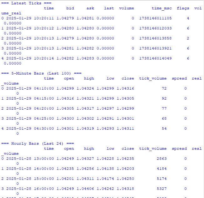
複雑な計算に入る前に、まずは取引ターミナルから正しくデータを取得できているかを確認しましょう。そのために、MetaTrader 5の動作確認とデータ構造の把握を目的とした、シンプルなテスト用スクリプトを用意しました。

import MetaTrader5 as mt5
import pandas as pd
from datetime import datetime, timedelta

pd.set_option('display.max_columns', 500)
pd.set_option('display.width', 1500)
pd.set_option('display.float_format', lambda x: '%.5f' % x)

def check_mt5_data(symbol="EURUSD"):
    if not mt5.initialize():
        print(f"MT5 initialization error: {mt5.last_error()}")
        return
    
    print("\n=== Symbol Information ===")
    symbol_info = mt5.symbol_info(symbol)
    if symbol_info is None:
        print(f"Failed to get {symbol} data")
        mt5.shutdown()
        return
    
    print(f"Current spread: {symbol_info.spread} points")
    print(f"Tick size: {symbol_info.trade_tick_size}")
    print(f"Contract size: {symbol_info.trade_contract_size}")
    
    # Last 100 ticks
    print("\n=== Latest Ticks ===")
    ticks = mt5.copy_ticks_from(symbol, datetime.now() - timedelta(minutes=5), 
                               100, mt5.COPY_TICKS_ALL)
    ticks_frame = pd.DataFrame(ticks)
    ticks_frame['time'] = pd.to_datetime(ticks_frame['time'], unit='s')
    print(ticks_frame.head())
    
    # 5-minute bars (last 100 bars)
    print("\n=== 5-Minute Bars (Last 100) ===")
    rates_5m = mt5.copy_rates_from_pos(symbol, mt5.TIMEFRAME_M5, 0, 100)
    rates_5m_frame = pd.DataFrame(rates_5m)
    rates_5m_frame['time'] = pd.to_datetime(rates_5m_frame['time'], unit='s')
    print(rates_5m_frame.head())
    
    # Hourly bars (last 24 hours)
    print("\n=== Hourly Bars (Last 24) ===")
    rates_1h = mt5.copy_rates_from_pos(symbol, mt5.TIMEFRAME_H1, 0, 24)
    rates_1h_frame = pd.DataFrame(rates_1h)
    rates_1h_frame['time'] = pd.to_datetime(rates_1h_frame['time'], unit='s')
    print(rates_1h_frame.head())
    
    # Daily bars (last 30 days)
    print("\n=== Daily Bars (Last 30) ===")
    rates_d1 = mt5.copy_rates_from_pos(symbol, mt5.TIMEFRAME_D1, 0, 30)
    rates_d1_frame = pd.DataFrame(rates_d1)
    rates_d1_frame['time'] = pd.to_datetime(rates_d1_frame['time'], unit='s')
    print(rates_d1_frame.head())
    
    # Statistics for different timeframes
    print("\n=== 5-Minute Bars Statistics ===")
    print(f"Average volume: {rates_5m_frame['tick_volume'].mean():.2f}")
    print(f"Average spread: {rates_5m_frame['spread'].mean():.2f}")
    print(f"Average range: {(rates_5m_frame['high'] - rates_5m_frame['low']).mean():.5f}")
    
    print("\n=== Hourly Bars Statistics ===")
    print(f"Average volume: {rates_1h_frame['tick_volume'].mean():.2f}")
    print(f"Average spread: {rates_1h_frame['spread'].mean():.2f}")
    print(f"Average range: {(rates_1h_frame['high'] - rates_1h_frame['low']).mean():.5f}")
    
    print("\n=== Daily Bars Statistics ===")
    print(f"Average volume: {rates_d1_frame['tick_volume'].mean():.2f}")
    print(f"Average spread: {rates_d1_frame['spread'].mean():.2f}")
    print(f"Average range: {(rates_d1_frame['high'] - rates_d1_frame['low']).mean():.5f}")
    
    # Current quotes
    print("\n=== Current Market Depth ===")
    depth = mt5.market_book_get(symbol)
    if depth is not None:
        bid = depth[0].price if depth[0].type == 1 else depth[1].price
        ask = depth[0].price if depth[0].type == 2 else depth[1].price
        print(f"Bid: {bid}")
        print(f"Ask: {ask}")
        print(f"Spread: {(ask - bid):.5f}")
    
    mt5.shutdown()

if __name__ == "__main__":
    check_mt5_data()

このコードは、接続の有効性と取得したデータの品質を確認するために必要な情報をすべて表示します。実行すると、以下の内容が確認できます。

• 取引銘柄に関する基本情報
• 最新のティックデータのテーブル
• 時間足バーのテーブル
• 出来高やスプレッドに関する統計情報
• 板情報から取得した現在のクォート

実行直後に、すべてが期待通りに動作していることがすぐに分かるはずです。どこかで問題が発生した場合でも、このスクリプトがどの段階でエラーが起きたのかを明確に示してくれます。

次のセクションでは、このデータを使って実際にボラティリティの計算をおこなっていきますが、その前に、データ取得の基盤が正しく機能していることを確認することが非常に重要です。

データ前処理

私が最初にボラティリティ予測に取り組み始めた頃は、一番重要なのはクールな機械学習モデルだと思っていました。しかし、実際に作業を進めていくうちにすぐ分かったのは、本当に重要なのはデータ前処理の品質だということです。ここでは、私がこの予測システムのために実際におこなっているデータ準備の考え方を紹介します。

私が使用している完全な前処理コードは次のとおりです。

import MetaTrader5 as mt5
import numpy as np
import pandas as pd
from sklearn.preprocessing import StandardScaler
from datetime import datetime, timedelta

pd.set_option('display.max_columns', 500)
pd.set_option('display.width', 1500)
pd.set_option('display.float_format', lambda x: '%.5f' % x)

class VolatilityProcessor:
    def __init__(self, lookback_periods=(5, 10, 20)):
        self.lookback_periods = lookback_periods
        self.scaler = StandardScaler()
        
    def calculate_volatility_features(self, df):
        df = df.copy()
        
        # Basic calculations
        df['returns'] = df['close'].pct_change().fillna(0)
        df['log_returns'] = (np.log(df['close']) - np.log(df['close'].shift(1))).fillna(0)
        
        # True Range
        df['true_range'] = np.maximum(
            df['high'] - df['low'],
            np.maximum(
                abs(df['high'] - df['close'].shift(1).fillna(df['high'])),
                abs(df['low'] - df['close'].shift(1).fillna(df['low']))
            )
        )
        
        # ATR and volatility
        for period in self.lookback_periods:
            df[f'atr_{period}'] = df['true_range'].rolling(window=period, min_periods=1).mean()
            df[f'volatility_{period}'] = df['returns'].rolling(window=period, min_periods=1).std()
        
        # Parkinson volatility
        df['parkinson_vol'] = np.sqrt(
            1/(4 * np.log(2)) * 
            np.power(np.log(df['high'].div(df['low'])), 2)
        )
        
        # Garman-Klass volatility
        df['garman_klass_vol'] = np.sqrt(
            0.5 * np.power(np.log(df['high'].div(df['low'])), 2) -
            (2*np.log(2)-1) * np.power(np.log(df['close'].div(df['open'])), 2)
        )
        
        # Relative volatility changes
        for period in self.lookback_periods:
            df[f'vol_change_{period}'] = (
                df[f'volatility_{period}'].div(df[f'volatility_{period}'].shift(1))
            )
            
        # Replace all infinities and NaN
        for col in df.columns:
            if df[col].dtype == float:
                df[col] = df[col].replace([np.inf, -np.inf], np.nan).fillna(0)
        
        return df
    
    def prepare_features(self, df):
        feature_cols = []
        
        # Time-based features - correct time conversion
        time = pd.to_datetime(df['time'], unit='s')
        
        # Hours (0-23) -> radians (0-2π)
        hours = time.dt.hour.values
        df['hour_sin'] = np.sin(2 * np.pi * hours / 24.0)
        df['hour_cos'] = np.cos(2 * np.pi * hours / 24.0)
        
        # Week days (0-6) -> radians (0-2π)
        days = time.dt.dayofweek.values
        df['day_sin'] = np.sin(2 * np.pi * days / 7.0)
        df['day_cos'] = np.cos(2 * np.pi * days / 7.0)
        
        # Select features
        for period in self.lookback_periods:
            feature_cols.extend([
                f'atr_{period}',
                f'volatility_{period}',
                f'vol_change_{period}'
            ])
        
        feature_cols.extend([
            'parkinson_vol', 
            'garman_klass_vol',
            'hour_sin',
            'hour_cos',
            'day_sin',
            'day_cos'
        ])
        
        # Create features DataFrame
        features = df[feature_cols].copy()
        
        # Final cleanup and scaling
        features = features.replace([np.inf, -np.inf], 0).fillna(0)
        scaled_features = self.scaler.fit_transform(features)
        
        return pd.DataFrame(
            scaled_features,
            columns=features.columns,
            index=features.index
        )
    
    def create_target(self, df, forward_window=12):
        future_vol = df['returns'].rolling(
            window=forward_window, min_periods=1, center=False
        ).std().shift(-forward_window).fillna(0)
        
        return future_vol

    def prepare_dataset(self, df, forward_window=12):
        print("\n=== Preparing Dataset ===")
        print("Initial shape:", df.shape)
        
        df = self.calculate_volatility_features(df)
        print("After calculating features:", df.shape)
        
        features = self.prepare_features(df)
        target = self.create_target(df, forward_window)
        
        print("Final shape:", features.shape)
        return features, target

def check_mt5_data(symbol="EURUSD"):
    if not mt5.initialize():
        print(f"MT5 initialization error: {mt5.last_error()}")
        return None
    
    rates = mt5.copy_rates_from_pos(symbol, mt5.TIMEFRAME_H1, 0, 10000)
    mt5.shutdown()
    
    if rates is None:
        return None
        
    return pd.DataFrame(rates)

def main():
    symbol = "EURUSD"
    rates_frame = check_mt5_data(symbol)
    
    if rates_frame is not None:
        print("\n=== Processing Hourly Data for Volatility Analysis ===")
        processor = VolatilityProcessor(lookback_periods=(5, 10, 20))
        features, target = processor.prepare_dataset(rates_frame)
        
        print("\nFeature statistics:")
        print(features.describe())
        print("\nFeature columns:", features.columns.tolist())
        print("\nTarget statistics:")
        print(target.describe())
    else:
        print("Failed to process data: MT5 data retrieval error")

if __name__ == "__main__":
    main()

しくみ

まず、MetaTrader 5から直近10,000本のH1（1時間）足を取得します。なぜこんなに多いかというと、試行錯誤の結果、これが最適な量だと分かったからです。学習には十分なデータ量でありながら、市場環境が大きく変わりすぎない範囲に収まります。

ここからが最も興味深い部分です。VolatilityProcessorクラスが、データ準備に関するすべての処理を担います。その内部では、次のような処理がおこなわれています。

1. まず、基本的なボラティリティ指標の計算です。ここでは3種類のボラティリティを扱います。
   • リターンの標準偏差という、最もクラシックなボラティリティ指標
   • True RangeやATRといった古典的でも今でも十分に有効な手法
   • 特にイントラデイの値動きを捉えるのに優れているParkinsonやGarman&Klassの手法
2. 時間情報の扱い方：時間帯や曜日をワンホットエンコーディングする代わりに、私はサイン波とコサイン波を使用します。これは単なる見せびらかしではありません。23:00と0:00が時間的に近いことを、モデルに正しく理解させるための重要な工夫です。
3. データの正規化とクリーニング：これはパイプライン全体の中で最も重要な工程です。
   • 外れ値や無限値を除去する
   • データの分布を歪めないことを慎重に確認したうえで、欠損値を0で補完する
   • すべての特徴量を同じ数値レンジにスケーリングする

その結果、最終的に15個の特徴量が得られます。これが本タスクにおける最適な数でした。より多くの特徴量（さまざまな特殊指標など）も試しましたが、実際には精度が悪化するだけでした。

目的変数は、将来12期間分のボラティリティです。なぜ12なのかというと、1時間足データでは約半日先の予測に相当し、取引判断には十分でありながら、予測として意味を失わない時間幅だからです。

注意すべき点

1. ローリング演算では、すべての箇所でmin_periods=1を使用しています。これは、時系列の先頭部分でデータが欠落してしまうのを防ぐためです。
2. 通常の「/」演算子ではなく「.div()」を使っているのは、単なる好みではありません。pandasはこの方法の方が、ゼロ除算などのエッジケースをより安全に処理してくれるからです。
3. 無限大値の置換は、各処理ステージの最後にまとめておこなっています。こうすることで、どの処理段階で問題が発生しているのかを見逃さずに済みます。

次のセクションでは、このように前処理されたデータを使って機械学習モデルを構築していきます。ただし、どれほど高度で洗練されたモデルを使ったとしても、前処理が不十分なデータを救うことはできない、という点を忘れないでください。

機械学習モデルの作成

さて、いよいよ最も興味深い部分、予測モデルの作成に入ります。最初に私が選んだのは、いかにも王道なアプローチでした。将来のボラティリティの正確な値を予測するための回帰モデルです。考え方はとても単純で、具体的な数値を予測し、それに何らかの係数を掛ければ、そのままストップロス水準に使える、というものでした。

最初の試み：回帰モデル

最初は、できるだけシンプルなコードから始めました。設定も最小限のXGBRegressorです。パラメータは、木の数が100、学習率が0.1、深さが5でした。今思えば、これで十分だと考えたのはかなり楽観的でしたが、誰しも最初はこうした遠回りをするものです。

結果は、控えめに言っても芳しくありませんでした。決定係数(R²)はおよそ0.05〜0.06に留まり、モデルが説明できているのはデータ変動のわずか5〜6%に過ぎませんでした。さらに、予測値の標準偏差は実際の値のほぼ3分の1程度しかなく、明らかに変動を捉えきれていませんでした。一方で、平均絶対誤差(MAE)は一見すると悪くない数値に見えました。

import MetaTrader5 as mt5
import numpy as np
import pandas as pd
from sklearn.preprocessing import StandardScaler
from sklearn.model_selection import TimeSeriesSplit
import xgboost as xgb
from xgboost import XGBRegressor
from sklearn.metrics import mean_squared_error, mean_absolute_error, r2_score
import matplotlib.pyplot as plt
from datetime import datetime, timedelta

# VolatilityProcessor class remains unchanged
class VolatilityProcessor:
    def __init__(self, lookback_periods=(5, 10, 20)):
        self.lookback_periods = lookback_periods
        self.scaler = StandardScaler()
        
    def calculate_volatility_features(self, df):
        df = df.copy()
        
        # Basic calculations
        df['returns'] = df['close'].pct_change().fillna(0)
        df['log_returns'] = (np.log(df['close']) - np.log(df['close'].shift(1))).fillna(0)
        df['abs_returns'] = abs(df['returns'])
        
        # Price changes
        df['price_range'] = (df['high'] - df['low']) / df['close']
        df['price_change'] = (df['close'] - df['open']) / df['open']
        
        # True Range
        df['true_range'] = np.maximum(
            df['high'] - df['low'],
            np.maximum(
                abs(df['high'] - df['close'].shift(1).fillna(df['high'])),
                abs(df['low'] - df['close'].shift(1).fillna(df['low']))
            )
        )
        
        # ATR and volatility for different periods
        for period in self.lookback_periods:
            # Standard features
            df[f'atr_{period}'] = df['true_range'].rolling(window=period, min_periods=1).mean()
            df[f'volatility_{period}'] = df['returns'].rolling(window=period, min_periods=1).std()
            
            # Additional rolling statistics
            df[f'mean_range_{period}'] = df['price_range'].rolling(window=period, min_periods=1).mean()
            df[f'mean_price_change_{period}'] = df['price_change'].rolling(window=period, min_periods=1).mean()
            df[f'max_price_change_{period}'] = df['price_change'].rolling(window=period, min_periods=1).max()
            df[f'min_price_change_{period}'] = df['price_change'].rolling(window=period, min_periods=1).min()
        
        # Advanced volatility measures
        # Parkinson volatility
        df['parkinson_vol'] = np.sqrt(
            1/(4 * np.log(2)) * 
            np.power(np.log(df['high'].div(df['low'])), 2)
        )
        
        # Garman-Klass volatility
        df['garman_klass_vol'] = np.sqrt(
            0.5 * np.power(np.log(df['high'].div(df['low'])), 2) -
            (2*np.log(2)-1) * np.power(np.log(df['close'].div(df['open'])), 2)
        )
        
        # Rogers-Satchell volatility
        df['rogers_satchell_vol'] = np.sqrt(
            np.log(df['high'].div(df['close'])) * np.log(df['high'].div(df['open'])) +
            np.log(df['low'].div(df['close'])) * np.log(df['low'].div(df['open']))
        )
        
        # Relative changes
        for period in self.lookback_periods:
            df[f'vol_change_{period}'] = (
                df[f'volatility_{period}'].div(df[f'volatility_{period}'].shift(1))
            )
            df[f'atr_change_{period}'] = (
                df[f'atr_{period}'].div(df[f'atr_{period}'].shift(1))
            )
            
        # Replace all infinities and NaN
        for col in df.columns:
            if df[col].dtype == float:
                df[col] = df[col].replace([np.inf, -np.inf], np.nan).fillna(0)
        
        return df
    
    def prepare_features(self, df):
        feature_cols = []
        
        # Time-based features
        time = pd.to_datetime(df['time'], unit='s')
        
        # Hours (0-23) -> radians (0-2π)
        hours = time.dt.hour.values
        df['hour_sin'] = np.sin(2 * np.pi * hours / 24.0)
        df['hour_cos'] = np.cos(2 * np.pi * hours / 24.0)
        
        # Days of week (0-6) -> radians (0-2π)
        days = time.dt.dayofweek.values
        df['day_sin'] = np.sin(2 * np.pi * days / 7.0)
        df['day_cos'] = np.cos(2 * np.pi * days / 7.0)
        
        # Select features
        for period in self.lookback_periods:
            feature_cols.extend([
                f'atr_{period}',
                f'volatility_{period}',
                f'vol_change_{period}'
            ])
        
        feature_cols.extend([
            'parkinson_vol', 
            'garman_klass_vol',
            'hour_sin',
            'hour_cos',
            'day_sin',
            'day_cos'
        ])
        
        # Create features DataFrame
        features = df[feature_cols].copy()
        
        # Final cleanup and scaling
        features = features.replace([np.inf, -np.inf], 0).fillna(0)
        scaled_features = self.scaler.fit_transform(features)
        
        return pd.DataFrame(
            scaled_features,
            columns=feature_cols,
            index=features.index
        )
    
    def create_target(self, df, forward_window=12):
        """Create target with log transformation"""
        future_vol = df['returns'].rolling(
            window=forward_window, min_periods=1, center=False
        ).std().shift(-forward_window)
        
        # Add small constant to avoid log(0)
        log_vol = np.log(future_vol + 1e-10)
        
        return log_vol.fillna(log_vol.mean())

    def prepare_dataset(self, df, forward_window=12):
        print("\n=== Preparing Dataset ===")
        print("Initial shape:", df.shape)
        
        df = self.calculate_volatility_features(df)
        print("After calculating features:", df.shape)
        
        features = self.prepare_features(df)
        target = self.create_target(df, forward_window)
        
        print("Final shape:", features.shape)
        return features, target

class VolatilityModel:
    def __init__(self, lookback_periods=(5, 10, 20), forward_window=12):
        self.processor = VolatilityProcessor(lookback_periods)
        self.forward_window = forward_window
        self.model = XGBRegressor(
            n_estimators=500,
            learning_rate=0.05,
            max_depth=10,
            min_child_weight=1,
            subsample=0.8,
            colsample_bytree=0.8,
            gamma=0.1,
            reg_alpha=0.1,
            reg_lambda=1,
            random_state=42,
            n_jobs=-1,
            objective='reg:squarederror'  # Better for log-transformed targets
        )
        self.feature_importance = None
        
    def prepare_data(self, rates_frame):
        """Prepare data using our processor"""
        features, target = self.processor.prepare_dataset(rates_frame)
        return features, target
    
    def create_train_test_split(self, features, target, test_size=0.2):
        """Split data preserving time order"""
        split_idx = int(len(features) * (1 - test_size))
        
        X_train = features.iloc[:split_idx]
        X_test = features.iloc[split_idx:]
        y_train = target.iloc[:split_idx]
        y_test = target.iloc[split_idx:]
        
        return X_train, X_test, y_train, y_test
    
    def train(self, X_train, y_train, X_test, y_test):
        """Train model with validation"""
        print("\n=== Training Model ===")
        print("Training set shape:", X_train.shape)
        print("Test set shape:", X_test.shape)
        
        # Train the model
        eval_set = [(X_train, y_train), (X_test, y_test)]
        self.model.fit(
            X_train, 
            y_train,
            eval_set=eval_set,
            verbose=True
        )
        
        # Save feature importance
        importance = self.model.feature_importances_
        self.feature_importance = pd.DataFrame({
            'feature': X_train.columns,
            'importance': importance
        }).sort_values('importance', ascending=False)
        
        # Make predictions and evaluate
        predictions = self.predict(X_test)
        metrics = self.calculate_metrics(y_test, predictions)
        
        return metrics
    
    def calculate_metrics(self, y_true, y_pred):
        """Calculate model performance metrics with detailed R2"""
        # Basic metrics
        rmse = np.sqrt(mean_squared_error(y_true, y_pred))
        mae = mean_absolute_error(y_true, y_pred)
        
        # Manual R2 calculation for verification
        y_true_mean = np.mean(y_true)
        total_sum_squares = np.sum((y_true - y_true_mean) ** 2)
        residual_sum_squares = np.sum((y_true - y_pred) ** 2)
        r2_manual = 1 - (residual_sum_squares / total_sum_squares)
        
        # Stats for debugging
        metrics = {
            'RMSE': rmse,
            'MAE': mae,
            'R2 (sklearn)': r2_score(y_true, y_pred),
            'R2 (manual)': r2_manual,
            'RSS': residual_sum_squares,
            'TSS': total_sum_squares,
            'Mean Prediction': np.mean(y_pred),
            'Mean Actual': np.mean(y_true),
            'Std Prediction': np.std(y_pred),
            'Std Actual': np.std(y_true),
            'Min Prediction': np.min(y_pred),
            'Max Prediction': np.max(y_pred),
            'Min Actual': np.min(y_true),
            'Max Actual': np.max(y_true)
        }
        
        print("\nDetailed Metrics Analysis:")
        print(f"Total Sum of Squares (TSS): {total_sum_squares:.8f}")
        print(f"Residual Sum of Squares (RSS): {residual_sum_squares:.8f}")
        print(f"R2 components: 1 - ({residual_sum_squares:.8f} / {total_sum_squares:.8f})")
        
        return metrics
    
    def predict(self, features):
        """Get volatility predictions with inverse log transform"""
        log_predictions = self.model.predict(features)
        return np.exp(log_predictions) - 1e-10
    
    def plot_feature_importance(self):
        """Visualize feature importance"""
        plt.figure(figsize=(12, 6))
        plt.bar(
            self.feature_importance['feature'],
            self.feature_importance['importance']
        )
        plt.xticks(rotation=45)
        plt.title('Feature Importance')
        plt.tight_layout()
        plt.show()
    
    def plot_predictions(self, y_true, y_pred, title="Model Predictions"):
        """Visualize predictions vs actual values"""
        plt.figure(figsize=(15, 7))
        plt.plot(y_true.values, label='Actual', alpha=0.7)
        plt.plot(y_pred, label='Predicted', alpha=0.7)
        plt.title(title)
        plt.legend()
        plt.tight_layout()
        plt.show()

def check_mt5_data(symbol="EURUSD"):
    if not mt5.initialize():
        print(f"MT5 initialization error: {mt5.last_error()}")
        return None
    
    rates = mt5.copy_rates_from_pos(symbol, mt5.TIMEFRAME_H1, 0, 10000)
    mt5.shutdown()
    
    if rates is None:
        return None
        
    return pd.DataFrame(rates)

def main():
    # Get data
    symbol = "EURUSD"
    rates_frame = check_mt5_data(symbol)
    
    if rates_frame is not None:
        # Create and train model
        model = VolatilityModel(lookback_periods=(5, 10, 20), forward_window=12)
        features, target = model.prepare_data(rates_frame)
        
        # Split data
        X_train, X_test, y_train, y_test = model.create_train_test_split(
            features, target, test_size=0.2
        )
        
        # Train and evaluate
        metrics = model.train(X_train, y_train, X_test, y_test)
        print("\n=== Model Performance ===")
        for metric, value in metrics.items():
            print(f"{metric}: {value:.6f}")
        
        # Make predictions
        predictions = model.predict(X_test)
        
        # Visualize results
        model.plot_feature_importance()
        model.plot_predictions(y_test, predictions, "Volatility Predictions")
    else:
        print("Failed to process data: MT5 data retrieval error")

if __name__ == "__main__":
    main()

これは完全な落とし穴だったのです。それは、このモデルが単に平均値付近を予測することを学習してしまったからです。相場が静かな期間では、すべてがうまく機能しているように見えました。しかし、ひとたび本当の値動きが始まると、モデルはその変化をあっさりと見逃してしまったのです。

回帰モデル改善のための試行錯誤

その後、回帰モデルを改善するために何週間も費やしました。さまざまなニューラルネットワークの構造を試し、特徴量を次々と追加し、損失関数を変え、ハイパーパラメータを調整し続けました。正直なところ、完全に疲れ果てるまでやり尽くしました。

しかし、結果はほとんど変わりませんでした。うまくいった場合でも、R²を0.15〜0.20程度まで引き上げるのが精一杯です。その代償として、モデルは不安定になり、過学習を起こし、そして何よりも肝心な「急激なボラティリティ上昇の瞬間」を依然として捉えることができませんでした。

アプローチの再考

そこで、あるときふと気づいたのです。そもそも、なぜ正確なボラティリティの値が必要なのだろうか、と。トレーダーにとって、ボラティリティが0.00234なのか0.00256なのかは、実はどうでもいいことです。本当に重要なのは、それが通常よりも明らかに高くなるかどうかだけなのです。

こうして、問題を分類問題として捉え直すというアイデアが生まれました。具体的な数値を予測する代わりに、2つの状態を定義します。通常または低ボラティリティ（ラベル0）と、75パーセンタイルを超える高ボラティリティ（ラベル1）です。

なぜこれがより効果的だったのでしょうか。

まず、シグナルが格段に明確になりました。曖昧な数値予測ではなく、「ボラティリティの急上昇が来るかどうか」という明確な答えが得られるようになったのです。この形式は解釈しやすく、取引システムへの組み込みも非常に簡単でした。

次に、極端な値への対応力が向上しました。回帰モデルでは外れ値が平均に引き寄せられてぼやけてしまいますが、分類ではそれらが「高ボラティリティ」という明確なクラスとしてパターン化されました。

そして最後に、実用性が大きく向上しました。トレーダーに必要なのは行動を起こすための明確な合図です。連続的な数値に合わせて保護注文を微調整するよりも、2つの状態に応じて調整する方が、はるかに現実的で扱いやすいことが分かったのです。

import MetaTrader5 as mt5
import numpy as np
import pandas as pd
from sklearn.preprocessing import StandardScaler
import xgboost as xgb
from xgboost import XGBClassifier
from sklearn.metrics import accuracy_score, precision_score, recall_score, f1_score, confusion_matrix
import matplotlib.pyplot as plt
import seaborn as sns

class VolatilityProcessor:
    def __init__(self, lookback_periods=(5, 10, 20), volatility_threshold=75):
        """
        Args:
            lookback_periods: periods for feature calculation
            volatility_threshold: percentile for defining high volatility
        """
        self.lookback_periods = lookback_periods
        self.volatility_threshold = volatility_threshold
        self.scaler = StandardScaler()
        
    def calculate_features(self, df):
        df = df.copy()
        
        # Basic calculations
        df['returns'] = df['close'].pct_change()
        df['abs_returns'] = abs(df['returns'])
        
        # True Range
        df['true_range'] = np.maximum(
            df['high'] - df['low'],
            np.maximum(
                abs(df['high'] - df['close'].shift(1)),
                abs(df['low'] - df['close'].shift(1))
            )
        )
        
        # Signs of volatility
        for period in self.lookback_periods:
            # ATR
            df[f'atr_{period}'] = df['true_range'].rolling(window=period).mean()
            
            # Volatility
            df[f'volatility_{period}'] = df['returns'].rolling(period).std()
            
            # Extremes
            df[f'high_low_range_{period}'] = (
                (df['high'].rolling(period).max() - df['low'].rolling(period).min()) 
                / df['close']
            )
            
            # Volatility acceleration
            df[f'volatility_change_{period}'] = (
                df[f'volatility_{period}'] / df[f'volatility_{period}'].shift(1)
            )
        
        # Add sentiment indicators
        df['body_ratio'] = abs(df['close'] - df['open']) / (df['high'] - df['low'])
        df['upper_shadow'] = (df['high'] - df[['open', 'close']].max(axis=1)) / (df['high'] - df['low'])
        df['lower_shadow'] = (df[['open', 'close']].min(axis=1) - df['low']) / (df['high'] - df['low'])
        
        # Data clearing
        for col in df.columns:
            if df[col].dtype == float:
                df[col] = df[col].replace([np.inf, -np.inf], np.nan)
                df[col] = df[col].fillna(method='ffill').fillna(0)
                
        return df
    
    def prepare_features(self, df):
        # Select features for the model
        feature_cols = []
        
        # Add time features
        time = pd.to_datetime(df['time'], unit='s')
        df['hour_sin'] = np.sin(2 * np.pi * time.dt.hour / 24)
        df['hour_cos'] = np.cos(2 * np.pi * time.dt.hour / 24)
        df['day_sin'] = np.sin(2 * np.pi * time.dt.dayofweek / 7)
        df['day_cos'] = np.cos(2 * np.pi * time.dt.dayofweek / 7)
        
        # Collect all features
        for period in self.lookback_periods:
            feature_cols.extend([
                f'atr_{period}',
                f'volatility_{period}',
                f'high_low_range_{period}',
                f'volatility_change_{period}'
            ])
            
        feature_cols.extend([
            'body_ratio',
            'upper_shadow',
            'lower_shadow',
            'hour_sin',
            'hour_cos',
            'day_sin',
            'day_cos'
        ])
        
        # Create DataFrame with features
        features = df[feature_cols].copy()
        features = features.replace([np.inf, -np.inf], 0).fillna(0)
        
        # Scale features
        scaled_features = self.scaler.fit_transform(features)
        
        return pd.DataFrame(
            scaled_features,
            columns=feature_cols,
            index=features.index
        )
    
    def create_target(self, df, forward_window=12):
        """Creates a binary label: 1 for high volatility, 0 for low volatility"""
        # Calculate future volatility
        future_vol = df['returns'].rolling(
            window=forward_window, min_periods=1, center=False
        ).std().shift(-forward_window)
        
        # Determine the threshold for high volatility
        vol_threshold = np.nanpercentile(future_vol, self.volatility_threshold)
        
        # Create binary labels
        target = (future_vol > vol_threshold).astype(int)
        target = target.fillna(0)
        
        return target
    
    def prepare_dataset(self, df, forward_window=12):
        print("\n=== Preparing Dataset ===")
        print("Initial shape:", df.shape)
        
        df = self.calculate_features(df)
        print("After calculating features:", df.shape)
        
        features = self.prepare_features(df)
        target = self.create_target(df, forward_window)
        
        print("Final shape:", features.shape)
        print(f"Positive class ratio: {target.mean():.2%}")
        
        return features, target

class VolatilityClassifier:
    def __init__(self, lookback_periods=(5, 10, 20), forward_window=12, volatility_threshold=75):
        self.processor = VolatilityProcessor(lookback_periods, volatility_threshold)
        self.forward_window = forward_window
        
        self.model = XGBClassifier(
            n_estimators=200,
            max_depth=6,
            learning_rate=0.1,
            subsample=0.8,
            colsample_bytree=0.8,
            min_child_weight=1,
            gamma=0.1,
            reg_alpha=0.1,
            reg_lambda=1,
            scale_pos_weight=1,
            random_state=42,
            n_jobs=-1,
            eval_metric=['auc', 'error']
        )
        
        self.feature_importance = None
    
    def prepare_data(self, rates_frame):
        features, target = self.processor.prepare_dataset(rates_frame)
        return features, target
    
    def create_train_test_split(self, features, target, test_size=0.2):
        split_idx = int(len(features) * (1 - test_size))
        
        X_train = features.iloc[:split_idx]
        X_test = features.iloc[split_idx:]
        y_train = target.iloc[:split_idx]
        y_test = target.iloc[split_idx:]
        
        return X_train, X_test, y_train, y_test
    
    def train(self, X_train, y_train, X_test, y_test):
        print("\n=== Training Model ===")
        print("Training set shape:", X_train.shape)
        print("Test set shape:", X_test.shape)
        
        # Train the model
        eval_set = [(X_train, y_train), (X_test, y_test)]
        self.model.fit(
            X_train, 
            y_train,
            eval_set=eval_set,
            verbose=True
        )
        
        # Maintain the importance of features
        importance = self.model.feature_importances_
        self.feature_importance = pd.DataFrame({
            'feature': X_train.columns,
            'importance': importance
        }).sort_values('importance', ascending=False)
        
        # Evaluate the model
        predictions = self.predict(X_test)
        metrics = self.calculate_metrics(y_test, predictions)
        
        return metrics
    
    def calculate_metrics(self, y_true, y_pred):
        metrics = {
            'Accuracy': accuracy_score(y_true, y_pred),
            'Precision': precision_score(y_true, y_pred),
            'Recall': recall_score(y_true, y_pred),
            'F1 Score': f1_score(y_true, y_pred)
        }
        
        # Error matrix
        cm = confusion_matrix(y_true, y_pred)
        print("\nConfusion Matrix:")
        print(cm)
        
        return metrics
    
    def predict(self, features):
        return self.model.predict(features)
    
    def predict_proba(self, features):
        return self.model.predict_proba(features)
    
    def plot_feature_importance(self):
        plt.figure(figsize=(12, 6))
        plt.bar(
            self.feature_importance['feature'],
            self.feature_importance['importance']
        )
        plt.xticks(rotation=45, ha='right')
        plt.title('Feature Importance')
        plt.tight_layout()
        plt.show()
    
    def plot_confusion_matrix(self, y_true, y_pred):
        cm = confusion_matrix(y_true, y_pred)
        plt.figure(figsize=(8, 6))
        sns.heatmap(cm, annot=True, fmt='d', cmap='Blues')
        plt.title('Confusion Matrix')
        plt.ylabel('True Label')
        plt.xlabel('Predicted Label')
        plt.tight_layout()
        plt.show()

def check_mt5_data(symbol="EURUSD"):
    if not mt5.initialize():
        print(f"MT5 initialization error: {mt5.last_error()}")
        return None
    
    rates = mt5.copy_rates_from_pos(symbol, mt5.TIMEFRAME_H1, 0, 10000)
    mt5.shutdown()
    
    if rates is None:
        return None
        
    return pd.DataFrame(rates)

def main():
    symbol = "EURUSD"
    rates_frame = check_mt5_data(symbol)
    
    if rates_frame is not None:
        # Create and train the model
        model = VolatilityClassifier(
            lookback_periods=(5, 10, 20), 
            forward_window=12, 
            volatility_threshold=75
        )
        features, target = model.prepare_data(rates_frame)
        
        # Separate data
        X_train, X_test, y_train, y_test = model.create_train_test_split(
            features, target, test_size=0.2
        )
        
        # Train and evaluate
        metrics = model.train(X_train, y_train, X_test, y_test)
        print("\n=== Model Performance ===")
        for metric, value in metrics.items():
            print(f"{metric}: {value:.4f}")
        
        # Make predictions
        predictions = model.predict(X_test)
        
        # Visualize results
        model.plot_feature_importance()
        model.plot_confusion_matrix(y_test, predictions)
    else:
        print("Failed to process data: MT5 data retrieval error")

if __name__ == "__main__":
    main()

新しいモデルの結果

分類問題に切り替えたことで、結果は劇的に改善されました。適合率は約70％に達し、つまり高ボラティリティのシグナル10回のうち、7回は実際に相場が動いたことを意味します。再現率は約65％で、危険な瞬間の約3分の2を捕捉できている計算です。しかし何より重要なのは、モデルが実際の取引に応用可能になったことです。

モデルの基本構造が定まったところで、次のセクションでは、このモデルを実際の取引システムにどのように組み込むか、そしてそのシグナルを基にどのような具体的な取引判断ができるかを解説します。これがボラティリティ予測の世界への旅で最も興味深い部分になるでしょう。

このアプローチについてどう思いますか。もし実務で似たような手法を使ったことがある方がいらっしゃれば、どのようなボラティリティ指標が役に立ったかもぜひ知りたいです。

将来の極端なボラティリティ指標

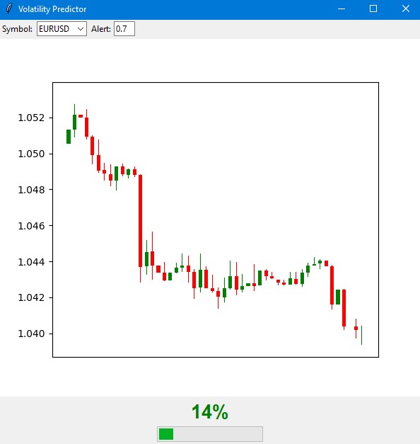
私が開発したインジケーターは、外国為替市場におけるボラティリティ急騰を予測するための総合ツールです。従来のボラティリティ指標が現在の状態を単に表示するのに対し、この指標は今後12時間の間に強い値動きが起こる可能性を予測します。

import tkinter as tk
from tkinter import ttk
import matplotlib
matplotlib.use('Agg')  # Important to install before importing pyplot
from matplotlib.figure import Figure
from matplotlib.backends.backend_tkagg import FigureCanvasTkAgg
import time
import MetaTrader5 as mt5

class VolatilityPredictor(tk.Tk):
   def __init__(self):
       super().__init__()
       self.title("Volatility Predictor")
       self.geometry("600x600")
       
       # Initialize the model
       self.model = VolatilityClassifier(
           lookback_periods=(5, 10, 20),
           forward_window=12,
           volatility_threshold=75
       )
       
       # Load and train the model at startup
       self.initialize_model()
       
       # Create the interface
       self.create_gui()
       
       # Launch the update
       self.update_data()
   
   def initialize_model(self):
       rates_frame = check_mt5_data("EURUSD")
       if rates_frame is not None:
           features, target = self.model.prepare_data(rates_frame)
           X_train, X_test, y_train, y_test = self.model.create_train_test_split(
               features, target, test_size=0.2
           )
           self.model.train(X_train, y_train, X_test, y_test)
   
   def create_gui(self):
       # Top panel with settings
       control_frame = ttk.Frame(self)
       control_frame.pack(fill='x', padx=2, pady=2)
       
       ttk.Label(control_frame, text="Symbol:").pack(side='left', padx=2)
       self.symbol_var = tk.StringVar(value="EURUSD")
       symbol_list = ["EURUSD", "GBPUSD", "USDJPY"]  # Simplified list
       ttk.Combobox(control_frame, textvariable=self.symbol_var, 
                   values=symbol_list, width=8).pack(side='left', padx=2)
       
       ttk.Label(control_frame, text="Alert:").pack(side='left', padx=2)
       self.threshold_var = tk.StringVar(value="0.7")
       ttk.Entry(control_frame, textvariable=self.threshold_var, 
                width=4).pack(side='left')
       
       # Chart
       self.fig = Figure(figsize=(6, 4), dpi=100)
       self.canvas = FigureCanvasTkAgg(self.fig, self)
       self.canvas.draw()
       self.canvas.get_tk_widget().pack(fill='both', expand=True, padx=2, pady=2)
       
       # Probability indicator
       gauge_frame = ttk.Frame(self)
       gauge_frame.pack(fill='x', padx=2, pady=2)
       
       self.probability_var = tk.StringVar(value="0%")
       self.probability_label = ttk.Label(
           gauge_frame, 
           textvariable=self.probability_var,
           font=('Arial', 20, 'bold')
       )
       self.probability_label.pack()
       
       self.progress = ttk.Progressbar(
           gauge_frame, 
           length=150,
           mode='determinate',
           maximum=100
       )
       self.progress.pack(pady=2)

   def update_data(self):
       try:
           rates = check_mt5_data(self.symbol_var.get())
           if rates is not None:
               features, _ = self.model.prepare_data(rates)
               probability = self.model.predict_proba(features)[-1][1]
               
               self.update_indicators(rates, probability)
               
               threshold = float(self.threshold_var.get())
               if probability > threshold:
                   self.alert(probability)
           
       except Exception as e:
           print(f"Error updating data: {e}")
       
       finally:
           self.after(1000, self.update_data)

   def update_indicators(self, rates, probability):
       self.fig.clear()
       ax = self.fig.add_subplot(111)
       
       df = rates.tail(50)  # Show fewer bars for compactness
       width = 0.6
       width2 = 0.1
       
       up = df[df.close >= df.open]
       down = df[df.close < df.open]
       
       ax.bar(up.index, up.close-up.open, width, bottom=up.open, color='g')
       ax.bar(up.index, up.high-up.close, width2, bottom=up.close, color='g')
       ax.bar(up.index, up.low-up.open, width2, bottom=up.open, color='g')
       
       ax.bar(down.index, down.close-down.open, width, bottom=down.open, color='r')
       ax.bar(down.index, down.high-down.open, width2, bottom=down.open, color='r')
       ax.bar(down.index, down.low-down.close, width2, bottom=down.close, color='r')
       
       ax.grid(False)  # Remove the grid for compactness
       ax.set_xticks([])  # Remove X axis labels
       self.canvas.draw()
       
       prob_pct = int(probability * 100)
       self.probability_var.set(f"{prob_pct}%")
       self.progress['value'] = prob_pct
       
       if prob_pct > 70:
           self.probability_label.configure(foreground='red')
       elif prob_pct > 50:
           self.probability_label.configure(foreground='orange')
       else:
           self.probability_label.configure(foreground='green')

   def alert(self, probability):
       window = tk.Toplevel(self)
       window.title("Alert!")
       window.geometry("200x80")  # Reduced alert window
       
       msg = f"High volatility: {probability:.1%}"
       ttk.Label(window, text=msg, font=('Arial', 10)).pack(pady=10)
       ttk.Button(window, text="OK", command=window.destroy).pack()

def main():
   app = VolatilityPredictor()
   app.mainloop()

if __name__ == "__main__":
   main()

インジケーターのメインウィンドウは、主に3つの部分に分かれています。上部には直近100本のローソク足チャートが表示され、現在の価格動向を視覚的に確認できます。緑色のローソクは上昇、赤色のローソクは下降を表し、従来通りの表示方法です。

中央部分には、インジケーターの主要要素である半円形の確率スケールが配置されています。ここでは、ボラティリティ急騰の現在の発生確率を0％から100％の範囲で示します。インジケーターの矢印はリスクレベルに応じて色が変化します。低リスク（50％以下）は緑、中リスク（50％～70％）はオレンジ、高リスク（70％以上）は赤で表示されます。

予測は、現在の市場状況と過去のボラティリティパターンの分析に基づいておこなわれます。モデルは直近20本のバーのデータを考慮して予測を構築し、今後12時間の間にボラティリティが増加する可能性を示します。信号発生後、最初の4～6時間で最も高い予測精度が得られます。

低確率（緑ゾーン）の場合、市場は落ち着いた動きを維持する可能性が高く、通常の取引システム設定で問題ありません。この期間は、標準のストップロス水準を利用することができます。

確率が中程度で矢印がオレンジに変わった場合は、注意を強化する必要があります。このタイミングでは、保護注文を標準サイズの約1/4増やすことが推奨されます。

確率が高く矢印が赤に変わった場合は、リスク管理を本格的に見直す必要があります。この期間は、ストップロスを少なくとも1.5倍に引き上げること、場合によっては状況が安定するまで新規ポジションの建玉を控えることが推奨されます。

インジケーターのコントロール要素は下部パネルに配置されています。ここでは、取引銘柄や時間足の選択、通知を受け取る閾値の設定が可能です。デフォルトでは閾値は70％に設定されており、シグナル数と信頼性のバランスを取る最適値です。

高ボラティリティシグナルにおける予測精度は70％に達します。つまり、急騰の可能性があると警告された10回のうち、7回は実際に発生します。また、インジケーターはすべての重要な値動きの約3分の2を捉えることができます。

重要なのは、このインジケーターは価格の方向性を予測するものではなく、あくまでボラティリティの上昇可能性を示すものである点です。主な目的は、トレーダーに強い値動きの可能性を事前に警告し、取引戦略や保護注文の水準を調整できるようにすることです。

将来的には、予測されたボラティリティに応じてストップロスを自動調整する機能の追加も予定されています。これにより、リスク管理プロセスがさらに自動化され、より安全に取引できるようになります。

このインジケーターは既存の取引システムを補完する形で活用でき、リスク管理の追加フィルターとして機能します。最大の利点は、潜在的な急激な値動きを事前に警告できる点であり、トレーダーに準備と戦略調整の時間を与えることです。

結論

現代の取引において、ボラティリティの予測は依然として成功する取引の重要な課題の一つです。本記事で紹介した、単純な回帰モデルから高ボラティリティ分類器への道筋は、複雑な手法よりも単純な解決策の方が効果的な場合があることを示しています。開発されたシステムは、予測精度およそ70％を達成し、全ての重要な値動きの約3分の2を捉えています。

ここから導き出される主な結論は、実務で重要なのは未来のボラティリティの正確な値ではなく、その急騰の可能性をいかにタイムリーに警告できるか、という点です。作成したインジケーターはこの課題をうまく解決しており、トレーダーが取引戦略や保護注文の水準を事前に調整できるようにします。古典的な分析手法と最新の機械学習技術を組み合わせることで、市場リスク管理の新たな可能性が広がります。

成功の鍵は、アルゴリズムの複雑さではなく、問題の正しい定式化と高品質なデータ準備にあることが分かりました。このアプローチは、さまざまな取引銘柄や時間足に応用可能であり、取引をより安全で予測可能なものにします。