
MQL5에서 ONNX 모델을 사용하는 방법

소개
기사의 작성자는 주가 예측을 위한 CNN-LSTM 기반 모델(Wenjie Lu, Jiazheng Li, Yifan Li, Aijun Sun, Jingyang Wang,Complexity Magazine, vol. 2020, Article ID 6622927, 10페이지, 2020)에서 다양한 주가 예측 모델을 비교했습니다.
주가 데이터는 시계열의 특성을 가지고 있습니다.
동시에 시계열 데이터 간의 관계를 메모리 기능을 통해 분석할 수 있는 장점이 있는 머신러닝 장단기 기억(LSTM)을 기반으로 한 CNN-LSTM 기반의 주가 예측 방법을 제안합니다.
그 동안 우리는 MLP, CNN, RNN, LSTM, CNN-RNN 및 이외 기타 예측 모델을 사용하여 주가를 하나씩 예측합니다. 또한 이들 모델의 예측 결과를 분석하고 비교합니다.
본 연구에 활용된 데이터는 1991년 7월 1일부터 2020년 8월 31일까지의 일일 주가(7,127거래일 포함) 입니다.
과거의 데이터 측면에서 우리는 시가, 최고가, 최저가, 종가, 거래량, 회전율, 상승 및 하락, 변화 등 8가지 특성을 선택했습니다.
먼저 이전 10일간의 항목의 데이터에서 효율적으로 특징을 추출하기 위해 CNN을 채택합니다. 그리고 추출된 특징 데이터로 주가를 예측하기 위해 LSTM을 채택합니다.
실험 결과에 따르면 CNN-LSTM이 가장 높은 예측 정확도로 신뢰할 수 있는 주가 예측을 제공할 수 있습니다.
이러한 예측 방법은 주가 예측을 위한 새로운 연구 아이디어를 제공할 뿐만 아니라 학자들에게 금융 시계열 데이터를 연구할 수 있는 실질적인 경험을 제공합니다.
살펴본 모든 모델 중에서는 CNN-LSTM 모델이 실험 중에 가장 좋은 결과를 생성했습니다. 이 기사에서는 금융 시계열을 예측하기 위해 이러한 모델을 생성하는 방법과 MQL5 Expert Advisor에서 생성된 ONNX 모델을 사용하는 방법에 대해 알아볼 것입니다.
1. 모델 구축
Python은 전문화된 라이브러리 세트를 제공하므로 ML 모델 작업을 위한 광범위한 기능을 제공합니다. 라이브러리는 데이터 준비 및 처리를 빠르게 해 줍니다.
ML 프로젝트의 효율성을 극대화하려면 GPU 리소스를 사용하는 것이 좋습니다. 많은 Windows 사용자가 현재 TensorFlow 버전을 설치하는 데 문제가 발생했습니다(비디오 가이드및 해당의 댓글 참조). master/install/manual_setup2.ipynb 텍스트 버전 ). 우리는 TensorFlow 2.10.0을 테스트했으며 이 버전을 사용하는 것이 좋습니다. GPU 계산은 CUDA 11.2 및 CUDNN 8.1.0.7 라이브러리를 사용하여 NVIDIA GeForce RTX 2080 Ti 그래픽 카드에서 수행되었습니다.
1.1. Python 및 라이브러리 설치
Python이 없으면 설치해야 합니다. 우리는 버전 3.9.16을 사용했습니다.
또한 라이브러리를 설치하십시오(Conda/Anaconda를 사용하는 경우 Anaconda 프롬프트에서 다음 명령을 실행하십시오):
python.exe -m pip install --upgrade pip
pip install --upgrade pandas
pip install --upgrade scikit-learn
pip install --upgrade matplotlib
pip install --upgrade tqdm
pip install --upgrade metatrader5
pip install --upgrade onnx==1.12
pip install --upgrade tf2onnx
pip install --upgrade tensorflow==2.10.0
1.2. TensorFlow 버전 및 GPU 확인
아래 코드는 설치된 TensorFlow 버전을 확인하고 GPU를 사용하여 모델을 계산할 수 있는지 여부를 확인합니다.
#check tensorflow version
print(tf.__version__)
#check GPU support
print(len(tf.config.list_physical_devices('GPU'))>0)
필요한 버전이 올바르게 설치된 경우 다음과 같은 결과가 표시됩니다.
True
우리는 Python 스크립트를 사용하여 모델을 구축하고 훈련했습니다. 이 프로세스의 각 단계는 아래에 간략하게 설명되어 있습니다.
1.3. 모델 구축 및 학습
스크립트는 모델에 사용될 Python 라이브러리를 가져오는 것으로 부터 시작됩니다.
#Python libraries
import matplotlib.pyplot as plt
import MetaTrader5 as mt5
import tensorflow as tf
import numpy as np
import pandas as pd
import tf2onnx
from sklearn.model_selection import train_test_split
from sys import argv
TensorFlow 버전 및 GPU 가용성을 확인하세요.
#check tensorflow version
print(tf.__version__)
2.10.0
#check GPU support
print(len(tf.config.list_physical_devices('GPU'))>0)
True
Python에서의 작업을 위해 MetaTrader 5를 초기화합니다.
#initialize MetaTrader5 for history data
if not mt5.initialize():
    print("initialize() failed, error code =",mt5.last_error())
    quit()
MetaTrader 5 터미널에 대한 정보:
#show terminal info
terminal_info=mt5.terminal_info()
print(terminal_info)
TerminalInfo(community_account=True, community_connection=True, connected=True, dlls_allowed=False, trade_allowed=False, tradeapi_disabled=False, email_enabled=False, ftp_enabled=False, notifications_enabled=False, mqid=False, build=3640, maxbars=100000, codepage=0, ping_last=58768, community_balance=1.0, retransmission=0.015296317559440137, company='MetaQuotes Software Corp.', name='MetaTrader 5', language='English', path='C:\\Program Files\\MetaTrader 5', data_path='C:\\Users\\user\\AppData\\Roaming\\MetaQuotes\\Terminal\\D0E8209F77C8CF37AD8BF550E51FF075', commondata_path='C:\\Users\\user\\AppData\\Roaming\\MetaQuotes\\Terminal\\Common')
#show file path
file_path=terminal_info.data_path+"\\MQL5\\Files\\"
print(file_path)
모델을 저장할 경로를 인쇄합니다(이 예에서는 스크립트가 Jupyter Notebook에서 실행됩니다).
#data path to save the model
data_path=argv[0]
last_index=data_path.rfind("\\")+1
data_path=data_path[0:last_index]
print("data path to save onnx model",data_path)
nx 모델을 저장할 데이터 경로 C:\Users\user\AppData\Roaming\Python\Python39\site-packages\
과거 데이터를 요청할 날짜를 준비하세요. 이 예에서는 현재 날짜부터 120에 대한 EURUSD H1 바를 요청합니다.
#set start and end dates for history data
from datetime import timedelta,datetime
end_date = datetime.now()
start_date = end_date - timedelta(days=120)

#print start and end dates
print("data start date=",start_date)
print("data end date=",end_date)
데이터 종료 날짜 = 2023-03-28 12:28:39.870685
EURUSD 과거 데이터 요청:
#get EURUSD rates (H1) from start_date to end_date
eurusd_rates = mt5.copy_rates_range("EURUSD", mt5.TIMEFRAME_H1, start_date, end_date)
다운로드한 데이터를 출력합니다.
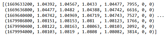
#check
print(eurusd_rates)
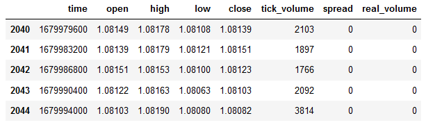
#create dataframe
df = pd.DataFrame(eurusd_rates)
dataframe의 시작과 끝을 표시합니다.
#show dataframe head
df.head()

#show dataframe tail
df.tail()
#show dataframe shape (the number of rows and columns in the data set)
df.shape
(2045, 8)
종가만 선택합니다.
#prepare close prices only
data = df.filter(['close']).values
데이터를 출력합니다:
#show close prices
plt.figure(figsize = (18,10))
plt.plot(data,'b',label = 'Original')
plt.xlabel("Hours")
plt.ylabel("Price")
plt.title("EURUSD_H1")
plt.legend()

MinMaxScaler를 사용하여 소스 가격 데이터를 [0,1] 범위로 조정합니다.
#scale data using MinMaxScaler
from sklearn.preprocessing import MinMaxScaler
scaler=MinMaxScaler(feature_range=(0,1))
scaled_data = scaler.fit_transform(data)
데이터의 처음 80%는 훈련에 사용됩니다.
#training size is 80% of the data
training_size = int(len(scaled_data)*0.80)
print("training size:",training_size)
훈련 사이즈: 1636
#create train data and check size
train_data_initial = scaled_data[0:training_size,:]
print(len(train_data_initial))
1636
#create test data and check size
test_data_initial= scaled_data[training_size:,:1]
print(len(test_data_initial))
409
다음 함수는 훈련 시퀀스를 생성합니다.
#split a univariate sequence into samples
def split_sequence(sequence, n_steps):
    X, y = list(), list()
    for i in range(len(sequence)):
       #find the end of this pattern
       end_ix = i + n_steps
       #check if we are beyond the sequence
       if end_ix > len(sequence)-1:
          break
       #gather input and output parts of the pattern
       seq_x, seq_y = sequence[i:end_ix], sequence[end_ix]
       X.append(seq_x)
       y.append(seq_y)
    return np.array(X), np.array(y)
세트를 구축하세요:
#split into samples
time_step = 120
x_train, y_train = split_sequence(train_data_initial, time_step)
x_test, y_test = split_sequence(test_data_initial, time_step)
#reshape input to be [samples, time steps, features] which is required for LSTM
x_train =x_train.reshape(x_train.shape[0],x_train.shape[1],1)
x_test = x_test.reshape(x_test.shape[0],x_test.shape[1],1)
훈련 및 테스트를 위한 Tensor 형태:
#show shape of train data
x_train.shape
(1516, 120, 1)
#show shape of test data
x_test.shape
(289, 120, 1)
#import keras libraries for the model
import math
from keras.models import Sequential
from keras.layers import Dense,Activation,Conv1D,MaxPooling1D,Dropout
from keras.layers import LSTM
from keras.utils.vis_utils import plot_model
from keras.metrics import RootMeanSquaredError as rmse
from keras import optimizers
모델을 설정합니다:
#define the model
model = Sequential()
model.add(Conv1D(filters=256, kernel_size=2,activation='relu',padding = 'same',input_shape=(120,1)))
model.add(MaxPooling1D(pool_size=2))
model.add(LSTM(100, return_sequences = True))
model.add(Dropout(0.3))
model.add(LSTM(100, return_sequences = False))
model.add(Dropout(0.3))
model.add(Dense(units=1, activation = 'sigmoid'))
model.compile(optimizer='adam', loss= 'mse' , metrics = [rmse()])
모델 속성을 표시합니다.
#show model
model.summary()

모델 훈련:
#measure time
import time
time_calc_start = time.time()

#fit model with 300 epochs
history=model.fit(x_train,y_train,epochs=300,validation_data=(x_test,y_test),batch_size=32,verbose=1)

#calculate time
fit_time_seconds = time.time() - time_calc_start
print("fit time =",fit_time_seconds," seconds.")
에포크 1/300
48/48 [===============================] - 8초 49ms/단계 - 손실: 0.0129 - root_mean_squared_error: 0.1136 - val_loss: 0.0065 - val_root_mean_squared_error: 0.0804
...
에포크 299/300
48/48 [==============================] - 2초 35ms/단계 - 손실: 4.5197e-04 - root_mean_squared_error: 0.0213 - val_loss: 4.2535e-04 - val_root_mean_squared_error: 0.0206
에포크 300/300
48/48 [===============================] - 2초 32ms/단계 - 손실: 4.2967e-04 - root_mean_squared_error: 0.0207 - val_loss: 4.4040e-04 - val_root_mean_squared_error: 0.0210
맞춤 시간 = 467.4918096065521초.
훈련하는 데에 약 8분 정도 소요되었습니다.
#show training history keys
history.history.keys()
훈련 및 테스트 데이터 세트의 최적화 역학:
#show iteration-loss graph for training and validation
plt.figure(figsize = (18,10))
plt.plot(history.history['loss'],label='Training Loss',color='b')
plt.plot(history.history['val_loss'],label='Validation-loss',color='g')
plt.xlabel("Iteration")
plt.ylabel("Loss")
plt.title("LOSS")
plt.legend()

#show iteration-rmse graph for training and validation
plt.figure(figsize = (18,10))
plt.plot(history.history['root_mean_squared_error'],label='Training RMSE',color='b')
plt.plot(history.history['val_root_mean_squared_error'],label='Validation-RMSE',color='g')
plt.xlabel("Iteration")
plt.ylabel("RMSE")
plt.title("RMSE")
plt.legend()

#evaluate training data
model.evaluate(x_train,y_train, batch_size = 32)
[0.00029911252204328775, 0.01729486882686615]
#evaluate testing data
model.evaluate(x_test,y_test, batch_size = 32)
10/10 [==============================] - 0초 31ms/단계 - 손실: 4.4040e-04 - root_mean_squared_error: 0.0210
[0.00044039846397936344, 0.020985672250390053]
훈련 데이터 세트에 대한 예측 형성:
#prediction using training data
train_predict = model.predict(x_train)
plot_y_train = y_train.reshape(-1,1)
훈련 간격에 대한 실제 및 예측 그래프를 출력합니다:
#show actual vs predicted (training) graph
plt.figure(figsize=(18,10))
plt.plot(scaler.inverse_transform(plot_y_train),color = 'b', label = 'Original')
plt.plot(scaler.inverse_transform(train_predict),color='red', label = 'Predicted')
plt.title("Prediction Graph Using Training Data")
plt.xlabel("Hours")
plt.ylabel("Price")
plt.legend()
plt.show()

테스트 데이터 세트에 대한 예측 형성:
#prediction using testing data
test_predict = model.predict(x_test)
plot_y_test = y_test.reshape(-1,1)
11/11 [===============================] - 0초 11ms/단계
측정 항목을 계산하려면 간격 [0,1]의 데이터를 변환해야 합니다. 이번에도 MinMaxScaler를 사용합니다.
#calculate metrics
from sklearn import metrics
from sklearn.metrics import r2_score
#transform data to real values
value1=scaler.inverse_transform(plot_y_test)
value2=scaler.inverse_transform(test_predict)
#calc score
score = np.sqrt(metrics.mean_squared_error(value1,value2))
print("RMSE         : {}".format(score))
print("MSE          :", metrics.mean_squared_error(value1,value2))
print("R2 score     :",metrics.r2_score(value1,value2))
RMSE: 0.0015151631684117558
MSE : 2.295719426911551e-06
R2 점수: 0.9683533377809039
#show actual vs predicted (testing) graph
plt.figure(figsize=(18,10))
plt.plot(scaler.inverse_transform(plot_y_test),color = 'b',  label = 'Original')
plt.plot(scaler.inverse_transform(test_predict),color='g', label = 'Predicted')
plt.title("Prediction Graph Using Testing Data")
plt.xlabel("Hours")
plt.ylabel("Price")
plt.legend()
plt.show()

모델을 onnx 파일로 내보냅니다.
# save model to ONNX
output_path = data_path+"model.eurusd.H1.120.onnx"
onnx_model = tf2onnx.convert.from_keras(model, output_path=output_path)
print(f"model saved to {output_path}")

output_path = file_path+"model.eurusd.H1.120.onnx"
onnx_model = tf2onnx.convert.from_keras(model, output_path=output_path)
print(f"saved model to {output_path}")

# finish
mt5.shutdown()
Python 스크립트의 전체 코드는 Jupyter Notebook의 글에 첨부되어 있습니다.
A CNN-LSTM-Based Model to Forecast Stock Price이란 글에서 CNN-LSTM 아키텍쳐를 사용한 모델에 대해 최상의 결과 R^2=0.9646을 얻었습니다. 우리의 경우 CNN-LSTM 네트워크는 R^2=0.9684라는 최상의 결과를 생성했습니다. 결과에 따르면 이러한 유형의 모델은 예측 문제를 해결하는 데 효율적일 수 있습니다.
우리는 금융 시계열을 예측하기 위해 CNN-LSTM 모델을 구축하고 훈련하는 Python 스크립트의 예를 살펴 보았습니다.
2. MetaTrader 5에서 모델 사용
2.1. 시작하기 전에 알아두면 좋은 것
모델을 생성하는 방법에는 두 가지가 있습니다. OnnxCreate를 사용하여 onnx 파일에서 모델을 생성하거나OnnxCreateFromBuffer를사용하여 데이터 배열에서 모델을 생성할 수 있습니다.
ONNX 모델이 EA의 리소스로 사용되는 경우에는 모델을 변경할 때마다 EA를 다시 컴파일해야 합니다.
모든 모델이 입력 및/또는 출력 텐서의 크기를 완전히 정의한 것은 아닙니다. 이는 일반적으로 패키지 크기를 담당하는 첫 번째 차원입니다. 모델을 실행하기 전에OnnxSetInputShape및OnnxSetOutputShape함수를 사용하여 크기를 명시적으로 지정해야 합니다. 모델의 입력 데이터는 모델을 훈련할 때와 동일한 방식으로 준비되어야 합니다.
입력 및 출력 데이터의 경우모델에서 사용되는것과 동일한 유형의 배열, 행렬 및/또는 벡터를 사용하는 것이 좋습니다. 이 경우 모델을 실행할 때 데이터를 변환할 필요가 없습니다. 원하는 형태로 데이터를 표현할 수 없는 경우자동으로 데이터가 변환됩니다.
OnnxRun을사용하여 모델을 추론(실행)합니다. 모델은 여러 번 실행될 수 있습니다. 모델을 사용한 후OnnxRelease함수를 사용하여 릴리즈 합니다.
2.2. onnx 파일 읽기 및 입력 및 출력에 대한 정보 가져오기
모델을 사용하려면 우리는 모델 위치, 입력 데이터 유형 및 모양, 출력 데이터 유형 및 모양을 알아야 합니다. 이전에 생성된 스크립트에 따르면 model.eurusd.H1.120.onnx는 onnx 파일을 생성한 Python 스크립트와 동일한 폴더에 있습니다. 입력은 float32, 120 정규화된 종가 입니다(배치 크기를 1로 사용하는 경우). 출력은 float32이며 이는 모델에서 예측한 하나의 정규화 된 가격입니다.
또한 우리는 MQL5 스크립트를 사용하여 모델 입력 및 출력 데이터를 얻기 위해 MQL5\Files 폴더에 onnx 파일을 생성했습니다.
//+------------------------------------------------------------------+
//|                                                OnnxModelInfo.mq5 |
//|                                  Copyright 2023, MetaQuotes Ltd. |
//|                                             https://www.mql5.com |
//+------------------------------------------------------------------+
#property copyright "Copyright 2023, MetaQuotes Ltd."
#property link      "https://www.mql5.com"
#property version   "1.00"

#define UNDEFINED_REPLACE 1

//+------------------------------------------------------------------+
//| Script program start function                                    |
//+------------------------------------------------------------------+
void OnStart()
  {
   string file_names[];
   if(FileSelectDialog("Open ONNX model",NULL,"ONNX files (*.onnx)|*.onnx|All files (*.*)|*.*",FSD_FILE_MUST_EXIST,file_names,NULL)<1)
      return;

   PrintFormat("Create model from %s with debug logs",file_names[0]);

   long session_handle=OnnxCreate(file_names[0],ONNX_DEBUG_LOGS);
   if(session_handle==INVALID_HANDLE)
     {
      Print("OnnxCreate error ",GetLastError());
      return;
     }

   OnnxTypeInfo type_info;

   long input_count=OnnxGetInputCount(session_handle);
   Print("model has ",input_count," input(s)");
   for(long i=0; i<input_count; i++)
     {
      string input_name=OnnxGetInputName(session_handle,i);
      Print(i," input name is ",input_name);
      if(OnnxGetInputTypeInfo(session_handle,i,type_info))
         PrintTypeInfo(i,"input",type_info);
     }

   long output_count=OnnxGetOutputCount(session_handle);
   Print("model has ",output_count," output(s)");
   for(long i=0; i<output_count; i++)
     {
      string output_name=OnnxGetOutputName(session_handle,i);
      Print(i," output name is ",output_name);
      if(OnnxGetOutputTypeInfo(session_handle,i,type_info))
         PrintTypeInfo(i,"output",type_info);
     }

   OnnxRelease(session_handle);
  }
//+------------------------------------------------------------------+
//| PrintTypeInfo                                                    |
//+------------------------------------------------------------------+
void PrintTypeInfo(const long num,const string layer,const OnnxTypeInfo& type_info)
  {
   Print("   type ",EnumToString(type_info.type));
   Print("   data type ",EnumToString(type_info.element_type));

   if(type_info.dimensions.Size()>0)
     {
      bool   dim_defined=(type_info.dimensions[0]>0);
      string dimensions=IntegerToString(type_info.dimensions[0]);
      for(long n=1; n<type_info.dimensions.Size(); n++)
        {
         if(type_info.dimensions[n]<=0)
            dim_defined=false;
         dimensions+=", ";
         dimensions+=IntegerToString(type_info.dimensions[n]);
        }
      Print("   shape [",dimensions,"]");
      //--- not all dimensions defined
      if(!dim_defined)
         PrintFormat("   %I64d %s shape must be defined explicitly before model inference",num,layer);
      //--- reduce shape
      uint reduced=0;
      long dims[];
      for(long n=0; n<type_info.dimensions.Size(); n++)
        {
         long dimension=type_info.dimensions[n];
         //--- replace undefined dimension
         if(dimension<=0)
            dimension=UNDEFINED_REPLACE;
         //--- 1 can be reduced
         if(dimension>1)
           {
            ArrayResize(dims,reduced+1);
            dims[reduced++]=dimension;
           }
        }
      //--- all dimensions assumed 1
      if(reduced==0)
        {
         ArrayResize(dims,1);
         dims[reduced++]=1;
        }
      //--- shape was reduced
      if(reduced<type_info.dimensions.Size())
        {
         dimensions=IntegerToString(dims[0]);
         for(long n=1; n<dims.Size(); n++)
           {
            dimensions+=", ";
            dimensions+=IntegerToString(dims[n]);
           }
         string sentence="";
         if(!dim_defined)
            sentence=" if undefined dimension set to "+(string)UNDEFINED_REPLACE;
         PrintFormat("   shape of %s data can be reduced to [%s]%s",layer,dimensions,sentence);
        }
     }
   else
      PrintFormat("no dimensions defined for %I64d %s",num,layer);
  }
//+------------------------------------------------------------------+
파일 선택 창에서 MQL5\Files에 저장된 onnx 파일을 선택하고,OnnxCreate를사용하여 파일에서 모델을 생성하고 다음과 같은 정보를 얻었습니다.
Create model from model.eurusd.H1.120.onnx with debug logs
ONNX: Creating and using per session threadpools since use_per_session_threads_ is true
ONNX: Dynamic block base set to 0
ONNX: Initializing session.
ONNX: Adding default CPU execution provider.
ONNX: Total shared scalar initializer count: 0
ONNX: Total fused reshape node count: 0
ONNX: Removing NodeArg 'Gather_out0'. It is no longer used by any node.
ONNX: Removing NodeArg 'Gather_token_1_out0'. It is no longer used by any node.
ONNX: Total shared scalar initializer count: 0
ONNX: Total fused reshape node count: 0
ONNX: Removing initializer 'sequential/conv1d/Conv1D/ExpandDims_1:0'. It is no longer used by any node.
ONNX: Use DeviceBasedPartition as default
ONNX: Saving initialized tensors.
ONNX: Done saving initialized tensors
ONNX: Session successfully initialized.
model has 1 input(s)
0 input name is conv1d_input
   type ONNX_TYPE_TENSOR
   data type ONNX_DATA_TYPE_FLOAT
   shape [-1, 120, 1]
   0 input shape must be defined explicitly before model inference
   shape of input data can be reduced to [120] if undefined dimension set to 1
model has 1 output(s)
0 output name is dense
   type ONNX_TYPE_TENSOR
   data type ONNX_DATA_TYPE_FLOAT
   shape [-1, 1]
   0 output shape must be defined explicitly before model inference
   shape of output data can be reduced to [1] if undefined dimension set to 1
디버깅 모드가 활성화되었으므로
long session_handle=OnnxCreate(file_names[0],ONNX_DEBUG_LOGS);
ONNX 접두사가 있는 로그가 있습니다.
모델에는 실제로 하나의 입력과 하나의 출력이 있다는 것을 알 수 있습니다. 여기서는 입력 텐서의 첫 번째 차원과 출력 텐서의 첫 번째 차원이 정의되지 않습니다. 이러한 차원이 배치 크기를 담당한다고 가정합니다. 따라서 모델을 추론하기 전에 작업할 크기(OnnxSetInputShape및OnnxSetOutputShape)를 명시적으로 지정해야 합니다. 일반적으로 하나의 데이터 세트만 모델에 입력됩니다. 자세한 예는 다음 단락 "트레이딩 EA에서 ONNX 모델을 사용하는 예"에서 볼 수 있습니다.
데이터를 준비할 때 차원이 [1, 120, 1]인 배열을 사용할 필요는 없습니다. 우리는 1차원 배열이나 120개 요소로 구성된 벡터를 입력할 수 있습니다.
2.3. 트레이딩 EA에서 ONNX 모델을 사용하는 예
선언 및 정의
#include <Trade\Trade.mqh>

input double InpLots = 1.0;    // Lots amount to open position

#resource "Python/model.120.H1.onnx" as uchar ExtModel[]

#define SAMPLE_SIZE 120

long     ExtHandle=INVALID_HANDLE;
int      ExtPredictedClass=-1;
datetime ExtNextBar=0;
datetime ExtNextDay=0;
float    ExtMin=0.0;
float    ExtMax=0.0;
CTrade   ExtTrade;

//--- price movement prediction
#define PRICE_UP   0
#define PRICE_SAME 1
#define PRICE_DOWN 2
OnInit 기능
//+------------------------------------------------------------------+
//| Expert initialization function                                   |
//+------------------------------------------------------------------+
int OnInit()
  {
   if(_Symbol!="EURUSD" || _Period!=PERIOD_H1)
     {
      Print("model must work with EURUSD,H1");
      return(INIT_FAILED);
     }

//--- create a model from static buffer
   ExtHandle=OnnxCreateFromBuffer(ExtModel,ONNX_DEFAULT);
   if(ExtHandle==INVALID_HANDLE)
     {
      Print("OnnxCreateFromBuffer error ",GetLastError());
      return(INIT_FAILED);
     }

//--- since not all sizes defined in the input tensor we must set them explicitly
//--- first index - batch size, second index - series size, third index - number of series (only Close)
   const long input_shape[] = {1,SAMPLE_SIZE,1};
   if(!OnnxSetInputShape(ExtHandle,ONNX_DEFAULT,input_shape))
     {
      Print("OnnxSetInputShape error ",GetLastError());
      return(INIT_FAILED);
     }

//--- since not all sizes defined in the output tensor we must set them explicitly
//--- first index - batch size, must match the batch size of the input tensor
//--- second index - number of predicted prices (we only predict Close)
   const long output_shape[] = {1,1};
   if(!OnnxSetOutputShape(ExtHandle,0,output_shape))
     {
      Print("OnnxSetOutputShape error ",GetLastError());
      return(INIT_FAILED);
     }
//---
   return(INIT_SUCCEEDED);
  }
우리는 현재 심볼/차트주기 데이터를 사용하기 때문에 EURUSD, H1에 대해서만 작업합니다.
우리 모델은 EA에 리소스로 포함되어 있습니다. EA는 자체로 구동 가능하며 외부 onnx 파일을 읽을 필요가 없습니다. 모델은 리소스 배열에서 생성됩니다.
입력 및 출력 데이터 shape는 명시적으로 정의되어야 합니다.
OnTick 함수:
//+------------------------------------------------------------------+
//| Expert tick function                                             |
//+------------------------------------------------------------------+
void OnTick()
  {
//--- check new day
   if(TimeCurrent()>=ExtNextDay)
     {
      GetMinMax();
      //--- set next day time
      ExtNextDay=TimeCurrent();
      ExtNextDay-=ExtNextDay%PeriodSeconds(PERIOD_D1);
      ExtNextDay+=PeriodSeconds(PERIOD_D1);
     }

//--- check new bar
   if(TimeCurrent()<ExtNextBar)
      return;
//--- set next bar time
   ExtNextBar=TimeCurrent();
   ExtNextBar-=ExtNextBar%PeriodSeconds();
   ExtNextBar+=PeriodSeconds();
//--- check min and max
   double close=iClose(_Symbol,_Period,0);
   if(ExtMin>close)
      ExtMin=close;
   if(ExtMax<close)
      ExtMax=close;

//--- predict next price
   PredictPrice();
//--- check trading according to prediction
   if(ExtPredictedClass>=0)
      if(PositionSelect(_Symbol))
         CheckForClose();
      else
         CheckForOpen();
  }
우리는 새로운 하루의 시작을 정의합니다. 시작일은 120일 시퀀스의 Low 및 High의 값을 업데이트하여 120시간 시퀀스의 가격을 정규화 하는 데 사용됩니다. 모델은 우리가 입력 데이터를 준비할 때 따라야 하는 이러한 조건에서 훈련되었습니다.
//+------------------------------------------------------------------+
//| Get minimal and maximal Close for last 120 days                  |
//+------------------------------------------------------------------+
void GetMinMax(void)
  {
   vectorf close;
   close.CopyRates(_Symbol,PERIOD_D1,COPY_RATES_CLOSE,0,SAMPLE_SIZE);
   ExtMin=close.Min();
   ExtMax=close.Max();
  }
필요한 경우 하루 종일 Low 및 High를 수정할 수 있습니다.
예측 함수:
//+------------------------------------------------------------------+
//| Predict next price                                               |
//+------------------------------------------------------------------+
void PredictPrice(void)
  {
   static vectorf output_data(1);            // vector to get result
   static vectorf x_norm(SAMPLE_SIZE);       // vector for prices normalize

//--- check for normalization possibility
   if(ExtMin>=ExtMax)
     {
      ExtPredictedClass=-1;
      return;
     }
//--- request last bars
   if(!x_norm.CopyRates(_Symbol,_Period,COPY_RATES_CLOSE,1,SAMPLE_SIZE))
     {
      ExtPredictedClass=-1;
      return;
     }
   float last_close=x_norm[SAMPLE_SIZE-1];
//--- normalize prices
   x_norm-=ExtMin;
   x_norm/=(ExtMax-ExtMin);
//--- run the inference
   if(!OnnxRun(ExtHandle,ONNX_NO_CONVERSION,x_norm,output_data))
     {
      ExtPredictedClass=-1;
      return;
     }
//--- denormalize the price from the output value
   float predicted=output_data[0]*(ExtMax-ExtMin)+ExtMin;
//--- classify predicted price movement
   float delta=last_close-predicted;
   if(fabs(delta)<=0.00001)
      ExtPredictedClass=PRICE_SAME;
   else
     {
      if(delta<0)
         ExtPredictedClass=PRICE_UP;
      else
         ExtPredictedClass=PRICE_DOWN;
     }
  }
먼저 정규화할 수 있는지 확인합니다. 정규화는 MinMaxScaler Python 함수에서와 같이 구현됩니다.
#scale data
from sklearn.preprocessing import MinMaxScaler
scaler=MinMaxScaler(feature_range=(0,1))
scaled_data = scaler.fit_transform(data)
따라서 정규화 코드는 매우 간단하고 직관적입니다.
입력 데이터 및 결과 수신을 위한 벡터는 정적으로 구성됩니다. 이는 전체 프로그램 수명 동안 존재하는 재배치 불가능한 버퍼를 보장합니다. 따라서 ONNX 모델의 입력 및 출력 텐서는 모델을 실행할 때마다 다시 생성되지 않습니다.
핵심 함수는 OnnxRun입니다. ONNX_NO_CONVERSION 플래그는 입력 및 출력 데이터를 변환해서는 안 된다는 것을 나타냅니다. 왜냐하면 MQL5 부동 소수점 유형이 ONNX_DATA_TYPE_FLOAT와 정확히 일치하기 때문입니다. ONNX_DEBUG 플래그가 설정되지 않았습니다.
이 후 얻은 데이터를 예측 가격으로 비정규화하고 클래스를 결정합니다:가격이 올라갈지, 내려갈지, 변하지 않을지
거래 전략은 간단합니다. 매 시간이 시작될때 해당 시간이 끝날 때의 가격 예측을 체크합니다. 만약 예상 가격이 오르면 매수합니다. 모델이 하향 움직임을 예측하면 매도합니다.
//+------------------------------------------------------------------+
//| Check for open position conditions                               |
//+------------------------------------------------------------------+
void CheckForOpen(void)
  {
   ENUM_ORDER_TYPE signal=WRONG_VALUE;
//--- check signals
   if(ExtPredictedClass==PRICE_DOWN)
      signal=ORDER_TYPE_SELL;    // sell condition
   else
     {
      if(ExtPredictedClass==PRICE_UP)
         signal=ORDER_TYPE_BUY;  // buy condition
     }

//--- open position if possible according to signal
   if(signal!=WRONG_VALUE && TerminalInfoInteger(TERMINAL_TRADE_ALLOWED))
     {
      double price;
      double bid=SymbolInfoDouble(_Symbol,SYMBOL_BID);
      double ask=SymbolInfoDouble(_Symbol,SYMBOL_ASK);
      if(signal==ORDER_TYPE_SELL)
         price=bid;
      else
         price=ask;
      ExtTrade.PositionOpen(_Symbol,signal,InpLots,price,0.0,0.0);
     }
  }
//+------------------------------------------------------------------+
//| Check for close position conditions                              |
//+------------------------------------------------------------------+
void CheckForClose(void)
  {
   bool bsignal=false;
//--- position already selected before
   long type=PositionGetInteger(POSITION_TYPE);
//--- check signals
   if(type==POSITION_TYPE_BUY && ExtPredictedClass==PRICE_DOWN)
      bsignal=true;
   if(type==POSITION_TYPE_SELL && ExtPredictedClass==PRICE_UP)
      bsignal=true;

//--- close position if possible
   if(bsignal && TerminalInfoInteger(TERMINAL_TRADE_ALLOWED))
     {
      ExtTrade.PositionClose(_Symbol,3);
      //--- open opposite
      CheckForOpen();
     }
  }
이제 Strategy Tester에서 EA의 성과를 확인해 보겠습니다. 연초부터 EA를 테스트하려면 이전 데이터를 사용하여 모델을 학습해야 합니다. 따라서 테스트 기간과 겹치지 않도록 하기 위해 사용하지 않는 부분을 제거하고 학습 종료 날짜를 변경하는 방식으로 Python 스크립트를 약간 수정했습니다.
ONNX.eurusd.H1.120.Training.py 스크립트는 Python 하위 폴더에 있으며 MetaEditor에서 직접 실행됩니다. ONNX 결과 모델은 동일한 Python 하위 폴더에 저장되며 EA 컴파일 중에 리소스로 사용됩니다.
# Copyright 2023, MetaQuotes Ltd.
# https://www.mql5.com

# python libraries
import MetaTrader5 as mt5
import tensorflow as tf
import numpy as np
import pandas as pd
import tf2onnx

# input parameters
inp_model_name = "model.eurusd.H1.120.onnx"
inp_history_size = 120

if not mt5.initialize():
    print("initialize() failed, error code =",mt5.last_error())
    quit()

# we will save generated onnx-file near our script to use as resource
from sys import argv
data_path=argv[0]
last_index=data_path.rfind("\\")+1
data_path=data_path[0:last_index]
print("data path to save onnx model",data_path)

# set start and end dates for history data
from datetime import timedelta, datetime
#end_date = datetime.now()
end_date = datetime(2023, 1, 1, 0)
start_date = end_date - timedelta(days=inp_history_size)

# print start and end dates
print("data start date =",start_date)
print("data end date =",end_date)

# get rates
eurusd_rates = mt5.copy_rates_range("EURUSD", mt5.TIMEFRAME_H1, start_date, end_date)

# create dataframe
df = pd.DataFrame(eurusd_rates)

# get close prices only
data = df.filter(['close']).values

# scale data
from sklearn.preprocessing import MinMaxScaler
scaler=MinMaxScaler(feature_range=(0,1))
scaled_data = scaler.fit_transform(data)

# training size is 80% of the data
training_size = int(len(scaled_data)*0.80)
print("Training_size:",training_size)
train_data_initial = scaled_data[0:training_size,:]
test_data_initial = scaled_data[training_size:,:1]

# split a univariate sequence into samples
def split_sequence(sequence, n_steps):
    X, y = list(), list()
    for i in range(len(sequence)):
       # find the end of this pattern
       end_ix = i + n_steps
       # check if we are beyond the sequence
       if end_ix > len(sequence)-1:
          break
       # gather input and output parts of the pattern
       seq_x, seq_y = sequence[i:end_ix], sequence[end_ix]
       X.append(seq_x)
       y.append(seq_y)
    return np.array(X), np.array(y)

# split into samples
time_step = inp_history_size
x_train, y_train = split_sequence(train_data_initial, time_step)
x_test, y_test = split_sequence(test_data_initial, time_step)

# reshape input to be [samples, time steps, features] which is required for LSTM
x_train =x_train.reshape(x_train.shape[0],x_train.shape[1],1)
x_test = x_test.reshape(x_test.shape[0],x_test.shape[1],1)

# define model
from keras.models import Sequential
from keras.layers import Dense, Activation, Conv1D, MaxPooling1D, Dropout, Flatten, LSTM
from keras.metrics import RootMeanSquaredError as rmse
model = Sequential()
model.add(Conv1D(filters=256, kernel_size=2, activation='relu',padding = 'same',input_shape=(inp_history_size,1)))
model.add(MaxPooling1D(pool_size=2))
model.add(LSTM(100, return_sequences = True))
model.add(Dropout(0.3))
model.add(LSTM(100, return_sequences = False))
model.add(Dropout(0.3))
model.add(Dense(units=1, activation = 'sigmoid'))
model.compile(optimizer='adam', loss= 'mse' , metrics = [rmse()])

# model training for 300 epochs
history = model.fit(x_train, y_train, epochs = 300 , validation_data = (x_test,y_test), batch_size=32, verbose=2)

# evaluate training data
train_loss, train_rmse = model.evaluate(x_train,y_train, batch_size = 32)
print(f"train_loss={train_loss:.3f}")
print(f"train_rmse={train_rmse:.3f}")

# evaluate testing data
test_loss, test_rmse = model.evaluate(x_test,y_test, batch_size = 32)
print(f"test_loss={test_loss:.3f}")
print(f"test_rmse={test_rmse:.3f}")

# save model to ONNX
output_path = data_path+inp_model_name
onnx_model = tf2onnx.convert.from_keras(model, output_path=output_path)
print(f"saved model to {output_path}")

# finish
mt5.shutdown()
ONNX 모델 기반 EA 테스트
이제 Strategy Tester의 과거 데이터를 바탕으로 EA를 테스트해 보겠습니다. 모델을 훈련하는 데 사용한 것과 동일한 매개변수인 EURUSD 기호와 H1의 차트 주기를 지정합니다.
테스트 간격에는 훈련 기간이 포함되지 않으며 연초(2023년 1월 1일)부터 시작됩니다.

전략에 따르면 신호는 매 시간이 시작될 때 한 번 확인되므로(EA는새로운 바가 나타나는 것을 모니터링합니다) 따라서 틱 모델링 모드는 중요하지 않습니다. OnTick은 바 마다 한 번씩 테스터에서 처리됩니다.
//+------------------------------------------------------------------+
//| Expert tick function                                             |
//+------------------------------------------------------------------+
void OnTick()
  {
//--- check new day
   if(TimeCurrent()>=ExtNextDay)
     {
      GetMinMax();
      //--- set next day time
      ExtNextDay=TimeCurrent();
      ExtNextDay-=ExtNextDay%PeriodSeconds(PERIOD_D1);
      ExtNextDay+=PeriodSeconds(PERIOD_D1);
     }

//--- check new bar
   if(TimeCurrent()<ExtNextBar)
      return;
//--- set next bar time
   ExtNextBar=TimeCurrent();
   ExtNextBar-=ExtNextBar%PeriodSeconds();
   ExtNextBar+=PeriodSeconds();
//--- check min and max
   float close=(float)iClose(_Symbol,_Period,0);
   if(ExtMin>close)
      ExtMin=close;
   if(ExtMax<close)
      ExtMax=close;

//--- predict next price
   PredictPrice();
//--- check trading according to prediction
   if(ExtPredictedClass>=0)
      if(PositionSelect(_Symbol))
         CheckForClose();
      else
         CheckForOpen();
  }
이 처리를 통해 3개월 간의 테스트에 단 몇 초밖에 걸리지 않습니다. 아래는 결과입니다.

이제 시그널에 의한 포지션 진입 및 SL(Stop Loss) 또는 이익실현(TP)에 의한 청산이 가능하도록 거래 전략을 수정해 보겠습니다.
input double InpLots       = 1.0;    // Lots amount to open position
input bool   InpUseStops   = true;   // Use stops in trading
input int    InpTakeProfit = 500;    // TakeProfit level
input int    InpStopLoss   = 500;    // StopLoss level

//+------------------------------------------------------------------+
//| Check for open position conditions                               |
//+------------------------------------------------------------------+
void CheckForOpen(void)
  {
   ENUM_ORDER_TYPE signal=WRONG_VALUE;
//--- check signals
   if(ExtPredictedClass==PRICE_DOWN)
      signal=ORDER_TYPE_SELL;    // sell condition
   else
     {
      if(ExtPredictedClass==PRICE_UP)
         signal=ORDER_TYPE_BUY;  // buy condition
     }

//--- open position if possible according to signal
   if(signal!=WRONG_VALUE && TerminalInfoInteger(TERMINAL_TRADE_ALLOWED))
     {
      double price,sl=0,tp=0;
      double bid=SymbolInfoDouble(_Symbol,SYMBOL_BID);
      double ask=SymbolInfoDouble(_Symbol,SYMBOL_ASK);
      if(signal==ORDER_TYPE_SELL)
        {
         price=bid;
         if(InpUseStops)
           {
            sl=NormalizeDouble(bid+InpStopLoss*_Point,_Digits);
            tp=NormalizeDouble(ask-InpTakeProfit*_Point,_Digits);
           }
        }
      else
        {
         price=ask;
         if(InpUseStops)
           {
            sl=NormalizeDouble(ask-InpStopLoss*_Point,_Digits);
            tp=NormalizeDouble(bid+InpTakeProfit*_Point,_Digits);
           }
        }
      ExtTrade.PositionOpen(_Symbol,signal,InpLots,price,sl,tp);
     }
  }
//+------------------------------------------------------------------+
//| Check for close position conditions                              |
//+------------------------------------------------------------------+
void CheckForClose(void)
  {
//--- position should be closed by stops
   if(InpUseStops)
      return;

   bool bsignal=false;
//--- position already selected before
   long type=PositionGetInteger(POSITION_TYPE);
//--- check signals
   if(type==POSITION_TYPE_BUY && ExtPredictedClass==PRICE_DOWN)
      bsignal=true;
   if(type==POSITION_TYPE_SELL && ExtPredictedClass==PRICE_UP)
      bsignal=true;

//--- close position if possible
   if(bsignal && TerminalInfoInteger(TERMINAL_TRADE_ALLOWED))
     {
      ExtTrade.PositionClose(_Symbol,3);
      //--- open opposite
      CheckForOpen();
     }
  }
InpUseStop = true, 이는 SL 및 TP 수준이 포지션 진입 시에 설정됨을 의미합니다.

같은 기간 동안 SL/TP 수준으로 테스트한 결과:

EA의 전체 소스 코드와 학습된 모델(2023년 초까지)은 첨부 파일에 있습니다.
결론
기사에서는 MQL5 프로그램에서 ONNX 모델을 사용하는 데 어려움이 없다는 것을 보여줍니다. 실제로 모델을 적용하는 것이 가장 쉬운 부분이지만 적절한 ONNX 모델을 얻는 것이 훨씬 더 어려운 것입니다.
기사에 사용된 모델은 MQL5 언어를 사용하여 ONNX 모델로 작업하는 방법을 보여주기 위한 데모의 목적으로만 제공됩니다. 이 기사에 제시된 Expert Advisor는 실제 거래를 위한 것이 아닙니다.
MetaQuotes 소프트웨어 사를 통해 러시아어가 번역됨.
원본 기고글: https://www.mql5.com/ru/articles/12373
경고: 이 자료들에 대한 모든 권한은 MetaQuotes(MetaQuotes Ltd.)에 있습니다. 이 자료들의 전부 또는 일부에 대한 복제 및 재출력은 금지됩니다.

 Expert Advisor 개발 기초부터(23부): 새로운 주문 시스템(VI)
틀림: 레이블에는 클래스 값이 포함되고 텐서에는 확률이 포함됩니다. 따라서 출력 차원은 본질적으로 2,2이지만 구조가 반환되므로 1을 입력해야 합니다.
감사합니다
감사합니다
그것이 당신이 존중하지 않는 전처리의 목적입니다 :) 먼저 왕겨에서 알갱이를 분리 한 다음 분리 된 알갱이를 예측하도록 훈련시키는 것입니다.
전처리가 좋으면 출력도 쓰레기가 아닙니다.
이 스크립트를 최신 버전의 파이썬(3.10-3.12)에서 실행되도록 수정할 수 있나요?
3.9에서 실행하는 데 많은 문제가 있습니다.
tx