Brute force approach to patterns search (Part VI): Cyclic optimization

Contents

• Introduction
• Routine
• New optimization algorithm
• Most important optimization criterion
• Auto search for trading configurations
• Conclusion
• Links

Introduction

Considering the material from my the previous article, I can say that this is only a superficial description of all the functions that I introduced into my algorithm. They concern not only the complete automation of the EA creation, but also such important functions as complete automation of the optimization and selection of results with subsequent use for automatic trading, or the creation of more progressive EAs I am going to show a little later.

Thanks to the symbiosis of trading terminals, universal EAs and the algorithm itself, you can completely get rid of manual development, or, in the worst case, reduce the labor intensity of possible improvements by an order of magnitude provided that you have the necessary computing capabilities. In this article, I will start describing the most important aspects of these innovations.

Routine

The most important factor in creation and subsequent modifications of such solutions over time for me was understanding the possibility of ensuring maximum automation of routine actions. Routine actions, in this case, include all non-essential human work:

• Generation of ideas.
• Creating a theory.
• Writing a code according to the theory.
• Code correction.
• Constant EA re-optimization.
• Constant EA selection.
• EA maintenance.
• Working with the terminals.
• Experiments and practice.
• Other.

As you can see, the range of this routine is quite wide. I treat this precisely as a routine, because I was able to prove that all these things can be automated. I have provided a general list. It does not matter who you are – an algorithmic trader, a programmer, or both. It does not matter whether you know how to program or not. Even if you do not, then in any case you will encounter at least half of this list. I am not talking about cases when you bought an EA in the market, launched it on the chart and calmed down by pressing one button. This, of course, happens, albeit extremely rarely.

Understanding all this, first I had to automate the most evident things. I conceptually described all this optimization in a previous article. However, when you do something like this, you begin to understand how to improve the whole thing, based on the already implemented functionality. The main ideas in this regard for me were the following:

• Improving the optimization mechanism.
• Creation of a mechanism for merging EAs (merging bots).
• Correct architecture of the interaction paths of all components.

Of course, this is a pretty brief enumeration. I will describe everything in more detail. By improving optimization I mean a set of several factors at once. All this is thought through within the chosen paradigm for building the entire system:

• Speeding up optimization by eliminating ticks.
• Accelerating optimization by eliminating profit curve control between trading decision points.
• Improving the quality of optimization by introducing custom optimization criteria.
• Maximizing the forward period efficiency.

On this website Forum, you can still find ongoing debates about whether optimization is needed at all and what its benefits are. Previously, I had a rather clear attitude towards this action, largely due to the influence of individual forum and website users. Now this opinion does not bother me at all. As for optimization, it all depends on whether you know how to use it correctly and what your objectives are. If used correctly, this action gives the desired result. In general, it turns out that this action is extremely useful.

Many people do not like optimization. There are two objective reasons for that:

• Lack of understanding of the basics (why, what and how to do, how to select results and everything related to this, including lack of experience).
• Imperfection of optimization algorithms.

In fact, both factors reinforce each other. To be fair, the MetaTrader 5 optimizer is structurally impeccably executed, but it still needs many improvements in terms of optimization criteria and possible filters. So far, all this functionality is akin to children's sandbox. Few people think about how to achieve positive forward periods and, most importantly, how to control this process. I have been thinking about this for a long time. In fact, a fair share of the current article is to be devoted to this topic.

New optimization algorithm

In addition to the basic known evaluation criteria of any backtest, we can come up with some combined characteristics that can help multiply the value of any algorithm for more efficient selection of results and subsequent application of settings. The advantage of these characteristics is that they can speed up the process of finding working settings. To do this, I created some sort of a strategy tester report similar to that in MetaTrader:

figure 1

With this tool, I can choose the option I like with a simple click. By clicking, a setting is generated, which I can immediately take and move to the appropriate folder in the terminal, so that universal EAs can read and start trading on it. If I want, I can also click the button to generate an EA and it will be built in case I need a separate EA with the settings hardwired inside. There is also a profit curve, which is redrawn when you select the next option from the table.

Let's figure out what is counted in the table. The primary elements for calculating these characteristics are the following data:

1. Points: profit of the entire backtest in "_Point" of the corresponding instrument.
2. Orders: the number of completely open and closed orders (they follow each other in strict order, according to the rule "there can only be one open order").
3. Drawdown: balance drawdown.

Based on these values, the following trade characteristics are calculated:

• Math Waiting: mathematical expectation in points.
• P Factor: analogue of the profit factor normalized to the range [-1 ... 0 ... 1] (my criterion).
• Martingale: martingale applicability (my criterion).
• MPM Complex: a composite indicator of the previous three (my criterion).

Let's now see how these criteria are calculated:

equations 1

As you can see, all the criteria that I created are very simple and, most importantly, easy to understand. Due to the fact that the increase in each of the criteria indicates that the backtest result is better in terms of the probability theory, it becomes possible to multiply these criteria, as I did in the MPM Complex criterion. A common metric will more effectively sort results by their importance. In case of massive optimizations, it will allow you to retain more high-quality options and remove more low-quality ones, respectively.

Also, note that in these calculations everything happens in points. This has a positive effect on the optimization process. For calculations, strictly positive primary quantities are used, which are always calculated at the beginning. All the rest is calculated based on them. I think, it is worth listing these primary quantities that are not in the table:

• Points Plus: sum of profits of each profitable or zero order in points
• Points Minus: sum of the loss modules of each unprofitable order in points
• Drawdown: drawdown by balance (I calculate it in my own way)

The most interesting thing here is how drawdown is calculated. In our case, this is the maximum relative balance drawdown. Considering the fact that my testing algorithm refuses to monitor the funds curve, other types of drawdowns cannot be calculated. However, I think it would be useful to show how I calculate this drawdown:

figure 2

It is defined very simply:

1. Calculate the starting point of the backtest (the start of the first drawdown countdown).
2. If trading begins with profit, then we move this point upward following the growth of the balance, until the first negative value appears (it marks the beginning of the drawdown calculation).
3. Wait until the balance reaches the level of the reference point. After that, set it as a new reference point.
4. We return to the last section of the drawdown search and look for the lowest point on it (the amount of drawdown in this section is calculated from this point).
5. Repeat the entire process for the entire backtest or trading curve.

The last cycle will always remain unfinished. However, its drawdown is also taken into account, despite the fact that there is a potential for it to increase if the test continues. But this is not a particularly important thing here.

Most important optimization criterion

Now let's talk about the most important filter. In fact, this criterion is the most important when selecting optimization results. This criterion is not included in the functionality of the MetaTrader 5 optimizer which is a pity. So let me provide theoretical material so that everyone can reproduce this algorithm in their own code. In fact, this criterion is multifunctional for any type of trading and works for absolutely any profit curve, including sports betting, cryptocurrency and anything else you can think of. The criterion is as follows:

equations 2

Let's see what is inside this equation:

• N — number of completely open and closed trading positions throughout the entire backtest or trading section.
• B(i) — value of the balance line after the corresponding closed position "i".
• L(i) — straight line drawn from zero to the very last point of the balance (final balance).

We need to perform two backtests to calculate this parameter. The first backtest will calculate the final balance. After that, it will be possible to calculate the corresponding indicator saving the value of each balance point so that there is no need to make unnecessary calculations. Nevertheless, this calculation can be called a repeated backtest. This equation can be used in custom testers, which can be built into your EAs.

It is important to note that this indicator as a whole can be modified for greater understanding. For example, like this:

equations 3

This equation is more difficult in terms of perception and understanding. But from the practical point of view, such a criterion is convenient because the higher it is, the more our balance curve resembles a straight line. I touched on similar issues in previous articles, but did not explain the meaning behind them. Let's first look at the following figure:

figure 3

This figure shows a balance line and two curves: one of which relates to our equation (red), and the second for the following modified criterion (equations 11). I will show it further, but now let's focus on the equation.

If we imagine our backtest as a simple array of points with balances, then we can represent it as a statistical sample and apply probability theory equations to it. We will consider the straight line to be the model we are striving for, and the profit curve itself to be the real data flow that is striving for our model.

It is important to understand that the linearity factor indicates the reliability of the entire available set of trading criteria. In turn, higher reliability of the data may indicate a possible longer and better forward period (profitable trading in the future). Strictly speaking, initially I should have started considering such things with a consideration of random variables, but it seemed to me that such a presentation should make it easier to understand.

Let's create an alternative analogue of our linearity factor, taking into account possible random spikes. To do this, we will need to introduce a random variable convenient for us and its average for subsequent dispersion calculation:

equations 4

For better understanding, it should be clarified that we have "N" completely open and closed positions, which follow strictly one after another. This means that we have "N+1" points that connect these segments of the balance line. The zero point of all lines is common, so its data will distort the results in the direction of improvement, just like the last point. Therefore, we throw them out of the calculations, and we are left with "N-1" points we will perform calculations on.

The selection of expression for converting the arrays of values of two lines into one turned out to be very interesting. Please note the following fraction:

equations 5

The important thing here is that we divide everything by the final balance in all cases. Thus, we reduce everything to a relative value, which ensures the equivalence of the calculated characteristics for all tested strategies, without exception. It is no coincidence that the same fraction is present in the very first and simple criterion of the linearity factor, since it is built on the same consideration. But let's complete the construction of our alternative criterion. To do this, we can use such a well-known concept as dispersion:

equations 6

Dispersion is nothing more than the arithmetic mean of the squared deviation from the mean of the entire sample. I immediately substituted our random variables there, the expressions for which were defined above. An ideal curve has a mean deviation of zero and, as a consequence, the dispersion of a given sample will also be zero. Based on these data, it is easy to guess that this dispersion, due to its structure - the random variable used or the sample (as you wish) - can be used as an alternative linearity factor. Moreover, both criteria can be used in tandem to more effectively constrain the sample parameters, although, to be honest, I only use the first criterion.

Let’s look at a similar, more convenient criterion, which is also based on a new linearity factor that we have defined:

equations 7

As we can see, it is identical to a similar criterion, which is built on the basis of the first one (equations 2). However, these two criteria are far from the limit of what can be thought of. An obvious fact that speaks in favor of this consideration is that this criterion is too idealized and is more suitable for ideal models, and it will be extremely difficult to adjust an EA to achieve a more or less significant correspondence. I think, it is worth listing the negative factors that will be obvious some time after applying the equations:

1. Critical reduction in the number of trades (reduces the reliability of the results)
2. Rejection of the maximum number of efficient scenarios (depending on the strategy, the curve does not always tend to the straight line)

These shortcomings are very critical, since the goal is not to discard good strategies, but, on the contrary, to find new and improved criteria that are free of these shortcomings. These disadvantages can be completely or partially neutralized by introducing several preferred lines at once, each of which can be considered an acceptable or preferred model. To understand the new improved criterion, free of these shortcomings, you only need to understand the corresponding replacement:

equations 8

Then we can calculate the fit factor for each curve from the list:

equations 9

Similarly, we can also calculate an alternative criterion that takes into account random spikes for each of the curves:

equations 10

Then we will need to calculate the following:

equations 11

Here I introduce a criterion called the curve family factor. In fact, with this action, we simultaneously find the most similar curve for our trading curve and immediately find the factor of correspondence to it. The curve with the minimum matching factor is the closest to the real situation. We take its value as the value of the modified criterion, and, of course, the calculation can be done in two ways, depending on which of the two variations we like better.

This is all very cool, but here, as many have noticed, there are nuances related to the selection of such a family of curves. In order to correctly describe such a family, one can follow various considerations, but here are my thoughts:

• All curves should not have inflection points (each subsequent intermediate point should be strictly higher than the previous one).
• The curve should be concave (the steepness of the curve can either be constant or it can only increase).
• The concavity of the curve should be adjustable (for example, the amount of deflection should be adjusted using some relative value or percentage).
• Curve model simplicity (it is better to base the model on initially simple and understandable graphical models).

This is only the initial variation of this family of curves. It is possible to make more extensive variations taking into account all the desired configurations, which can completely save us from losing quality settings. I will take on this task later, but for now I will only touch on the original strategy of the family of concave curves. I was able to create such a family quite easily using my knowledge of math. Let me immediately show you what this family of curves ultimately looks like:

figure 4

When constructing such a family, I used the abstraction of an elastic rod that lies on vertical supports. The degree of deflection of such a rod depends on the point of application of the force and its magnitude. It is clear that this only somewhat resembles what we are dealing with here, but it is quite enough to develop some kind of visually similar model. In this situation, of course, we should first of all determine the coordinate of the extremum, which should coincide with one of the points on the back test chart, and there the X axis is represented by the trade indices starting from zero. I calculate it like this:

equations 12

There are two cases here: for even and odd "N". If "N" turns out to be even, then it is impossible to simply divide it by two, since the index should be an integer. By the way, I depicted exactly this case in the last picture. There, the point of application of force is a little closer to the beginning. You can, of course, do the opposite, a little closer to the end, but this will be significant only with a small number of trades, as I depicted in the figure. As the number of trades increases, all this will not play any significant role for optimization algorithms.

Having set the "P" deflection value in percentage and the "B" final balance of the backtest, having previously determined the coordinate of the extremum, we can begin to sequentially calculate further components to construct expressions for each of the accepted family of curves. Next we need the steepness of the straight line connecting the beginning and end of the backtest:

equations 13

Another feature of these curves is the fact that the angle tangent to each of the curves at points with the "N0" abscissa is identical to "K". When constructing equations, I required this condition from the task. This can also be seen graphically in the last figure (figure 4), and there are some equations and identities there too. Let's move on. Now we need to calculate the following value:

equations 14

 

Keep in mind that "P" is set differently for each curve from the family. Strictly speaking, these are equations for constructing one curve from a family. These calculations should be repeated for each curve from the family. Then we need to calculate another important ratio:

equations 15

There is no need to delve into the meaning of these structures. They are only created to simplify the process of constructing curves. It remains to calculate the last auxiliary ratio:

equations 16

Now, based on the data obtained, we can receive a mathematical expression for calculating the points of the constructed curve. However, it is first necessary to clarify that the curve is not described by a single equation. To the left of the "N0" point, we have one equation, while another one works to the right. To make it easier to understand, we can do the following:

equations 17

Now we can see the final equations:

equations 18

We can also show this as follows:

equations 19

Strictly speaking, this function should be used as a discrete and auxiliary function. But nevertheless, it allows us to calculate values in fractional "i". This, of course, is unlikely to have any useful benefits for us in the context of our problem.

Since I am giving such math, I am obliged to provide examples of the algorithm implementation. I think, everyone will be interested in getting ready-made code that will be easier to adapt to their systems. Let's start by defining the main variables and methods that will simplify the calculation of the necessary quantities:

//+------------------------------------------------------------------+
//| Number of lines in the balance model                             |
//+------------------------------------------------------------------+
#define Lines 11 

//+------------------------------------------------------------------+
//| Initializing variables                                           |
//+------------------------------------------------------------------+
double MaxPercent = 10.0;
double BalanceMidK[,Lines];
double Deviations[Lines];
int Segments;
double K;

//+------------------------------------------------------------------+
//| Method for initializing required variables and arrays            |
//| Parameters: number of segments and initial balance               |
//+------------------------------------------------------------------+
void InitLines(int SegmentsInput, double BalanceInput) 
{
  Segments = SegmentsInput;
  K = BalanceInput / Segments;
  ArrayResize(BalanceMidK,Segments+1);
  ZeroStartBalances();
  ZeroDeviations();
  BuildBalances();
}

//+------------------------------------------------------------------+
//| Resetting variables for incrementing balances                    |
//+------------------------------------------------------------------+
void ZeroStartBalances()
{
  for (int i = 0; i < Lines; i++ ) 
  {
      for (int j = 0; j <= Segments; j++)
      {
          BalanceMidK[j,i] = 0.0;
      }
  }
}

//+------------------------------------------------------------------+
//| Reset deviations                                                 |
//+------------------------------------------------------------------+
void ZeroDeviations()
{
  for (int i = 0; i < Lines; i++)
  {
      Deviations[i] = -1.0;
  }
}

The code is designed to be reusable. After the next calculation, you can calculate the indicator for a different balance curve by first calling the InitLines method. You need to give it the final balance of the backtest and the number of trades, after which you can start constructing our curves based on this data:

//+------------------------------------------------------------------+
//| Constructing all balances                                        |
//+------------------------------------------------------------------+
void BuildBalances()
{
   int N0 = MathFloor(Segments / 2.0) - Segments / 2.0 == 0 ? Segments / 2 : (int)MathFloor(Segments / 2.0);//calculate first required N0
   for (int i = 0; i < Lines; i++)
   {
       if (i==0)//very first and straight line 
       {
           for (int j = 0; j <= Segments; j++)
           {
               BalanceMidK[j,i] = K*j;
           }
       }
       else//build curved lines
       {
           double ThisP = i * (MaxPercent / 10.0);//calculate current line curvature percentage
           double KDelta = ( (ThisP /100.0) * K * Segments) / (MathPow(N0,2)/2.0 );//calculation first auxiliary ratio
           double Psi0 = -KDelta * N0;//calculation second auxiliary ratio
           double KDelta1 = ((ThisP / 100.0) * K * Segments) / (MathPow(Segments-N0, 2) / 2.0);//calculate last auxiliary ratio
           //this completes the calculation of auxiliary ratios for a specific line, it is time to construct it

           for (int j = 0; j <= N0; j++)//construct the first half of the curve 
           {
               BalanceMidK[j,i] = (K + Psi0 + (KDelta * j) / 2.0) * j;
           }
           for (int j = N0; j <= Segments; j++)//construct the second half of the curve 
           {
               BalanceMidK[j,i] = BalanceMidK[i, N0] + (K + (KDelta1 * (j-N0)) / 2.0) * (j-N0);
           }
       }
   }
}

Please note that "Lines" determines how many curves there will be in our family. The concavity gradually increases from zero (straight) and so on to MaxPercent, exactly as I showed in the corresponding figure. Then you can calculate the deviation for each of the curves and select the minimum one:

//+------------------------------------------------------------------+
//| Calculation of the minimum deviation from all lines              |
//| Parameters: initial balance passed via link                      |
//| Return: minimum deviation                                        |
//+------------------------------------------------------------------+
double CalculateMinDeviation(double &OriginalBalance[])
{
   //define maximum relative deviation for each curve 
   for (int i = 0; i < Lines; i++)
   {
       for (int j = 0; j <= Segments; j++)
       {
          double CurrentDeviation = OriginalBalance[Segments] ? MathAbs(OriginalBalance[j] - BalanceMidK[j, i]) / OriginalBalance[Segments] : -1.0;
          if (CurrentDeviation > Deviations[i])
          {
              Deviations[i] = CurrentDeviation;
          }           
       }
   }
    
   //determine curve with minimum deviation and deviation itself 
   double MinDeviation=0.0;
   for (int i = 0; i < Lines; i++)
   {
       if ( Deviations[i] != -1.0 && MinDeviation == 0.0)
       {
           MinDeviation = Deviations[i];
       }
       else if (Deviations[i] != -1.0 && Deviations[i] < MinDeviation)
       {
           MinDeviation = Deviations[i];
       }
   }
   return MinDeviation;
}

This is how we should use it:

1. Definition of the OriginalBalance original balance array.
2. Determine its length SegmentsInput and the final balance BalanceInput, as well as call the InitLines method.
3. Then we build the curves by calling the BuildBalances method.
4. Since the curves are plotted, we can consider our improved CalculateMinDeviation criterion for the family of curves.

This completes the calculation of the criterion. I think the calculation of the Curve Family Factor will not cause any difficulties. There is no need to present it here.

Auto search for trading configurations 

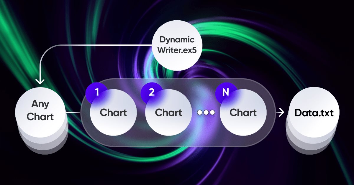
The most important element in the whole idea is the interaction system between the terminal and my program. In fact, it is a cyclic optimizer with advanced optimization criteria. The most important ones were covered in the previous section. In order for the entire system to function, we first need a source of quotes, which is one of the MetaTrader 5 terminals. As I already showed in the previous article, quotes are written to a file in a format that is convenient for me. This is done using an EA, which functions rather strangely at first glance:

.

I found it quite an interesting and beneficial experience to use my unique scheme for the EA functioning. Here is only a demonstration of the problems that I needed to solve, but all this can also be used for trading EAs:

 

The peculiarity of this scheme is that we choose any graph to choose from. It will not be used as a trading tool, in order to avoid duplication of data, but it will act only as a tick handler or timer. The rest of the charts represent those instruments-periods we need to generate quotes for.

Writing quotes is done in the form of a random selection of quotes using a random number generator. We can optimize this process if required. Writing occurs after a certain period of time using this basic function:

//+------------------------------------------------------------------+
//| Function to write data if present                                |
//| Write quotes to file                                             |
//+------------------------------------------------------------------+
void WriteDataIfPresent()
{
    // Declare array to store quotes 
    MqlRates rates[];
    ArraySetAsSeries(rates, false);

    // Select a random chart from those we added to the workspace 
    ChartData Chart = SelectAnyChart();
    
    // If the file name string is not empty 
    if (Chart.FileNameString != "")
    {
        // Copy quotes and calculate the real number of bars
        int copied = CopyRates(Chart.SymbolX, Chart.PeriodX, 1,
                        int((YearsE*(365.0*(5.0/7.0)*24*60*60)) / double(PeriodSeconds(Chart.PeriodX))),
                        rates);
        
        // Calculate ideal number of bars
        int ideal = int((YearsE*(365.0*(5.0/7.0)*24*60*60)) / double(PeriodSeconds(Chart.PeriodX)));
        
        // Calculate percentage of received data 
        double Percent = 100.0 * copied / ideal;
        
        // If the received data is not very different from the desired data, 
        // then we accept them and write them to a file
        if (Percent >= 95.0)
        {
            // Open file (create it if it does not exist, 
            // otherwise, erase all the data it contained)
            OpenAndWriteStart(rates, Chart, CommonE); 
            WriteAllBars(rates); // Write all data to file
            WriteEnd(rates); // Add to end
            CloseFile(); // Close and save data file
        }
        else 
        {
            // If there are much fewer quotes than required for calculation 
            Print("Not enough data"); 
        }
    }
}

The WriteDataIfPresent function writes information about quotes from the selected chart to a file if the copied data is at least 95% of the ideal number of bars calculated based on the specified parameters. If the copied data is less than 95%, the function displays the message "Not enough data". If a file with the given name does not exist, the function creates it.

For this code to function, the following should be additionally described:

//+------------------------------------------------------------------+
//| ChartData structure                                              |
//| Objective: Storing the necessary chart data                      |
//+------------------------------------------------------------------+
struct ChartData {
    string FileNameString;
    string SymbolX;
    ENUM_TIMEFRAMES PeriodX;
};

//+------------------------------------------------------------------+
//| Randomindex function                                             |
//| Objective: Get a random number with uniform distribution         |
//+------------------------------------------------------------------+
int Randomindex(int start, int end) {
    return start + int((double(MathRand())/32767.0)*double(end-start+1));
}

//+------------------------------------------------------------------+
//| SelectAnyChart function                                          |
//| Objective: View all charts except current one and select one of  |
//|       them to write quotes                                       |
//+------------------------------------------------------------------+
ChartData SelectAnyChart() {
    ChartData chosenChart;
    chosenChart.FileNameString = "";
    int chartCount = 0;
    long currentChartId, previousChartId = ChartFirst();

    // Calculate number of charts
    while (currentChartId = ChartNext(previousChartId)) {
        if(currentChartId < 0) {
            break;  
        }
        previousChartId = currentChartId;
        
        if (currentChartId != ChartID()) {
            chartCount++;
        }
    }

    int randomChartIndex = Randomindex(0, chartCount - 1);
    chartCount = 0;
    currentChartId = ChartFirst(); 
    previousChartId = currentChartId;
    
    // Select random chart
    while (currentChartId = ChartNext(previousChartId)) {
        if(currentChartId < 0) {
            break;
        }
        
        previousChartId = currentChartId;
        
        // Fill in selected chart data
        if (chartCount == randomChartIndex) {
            chosenChart.SymbolX = ChartSymbol(currentChartId);
            chosenChart.PeriodX = ChartPeriod(currentChartId);
            chosenChart.FileNameString = "DataHistory" + " " + chosenChart.SymbolX + " " + IntegerToString(CorrectPeriod(chosenChart.PeriodX));
        }
        
        if (chartCount > randomChartIndex) {
            break;
        }

        if (currentChartId != ChartID()) {
            chartCount++;
        }
    }
       
    return chosenChart;
}

This code is used to record and analyze historical financial market data (quotes) for different currencies from various charts that can be opened in the terminal at the moment.

• The ChartData structure is used to store data about each chart, including file name, symbol (currency pair) and timeframe. 
• The "Randomindex(start, end)" function generates a random number between "start" and "end". This is used to randomly select one of the available charts.
• SelectAnyChart() iterates through all open and available charts, excluding the current one, and then randomly selects one of them for processing.

The generated quotes are automatically picked up by the program, after which profitable configurations are automatically searched. Automating the entire process is quite complex, but I tried to condense it into one picture:

figure 5

There are three states of this algorithm:

1. Deactivated.
2. Waiting for quotes.
3. Active.

If the EA for recording quotes has not yet generated a single file or we have deleted all quotes from the specified folder, then the algorithm simply waits for them to appear and pauses for a while. As for our improved criterion, which I implemented for you in MQL5 style, it is also implemented for both brute force and optimization:

figure 6

The advanced mode operates the curve family factor, while the standard algorithm uses only the linearity factor. The remaining improvements are too extensive to fit into this article. In the next article I will show my new algorithm for gluing together advisors based on the universal multi-currency template. The template is launched on one chart, but processes all merged trading systems without requiring each EA to be launched on its own chart. Some of its functionality was used in this article.

Conclusion

In this article, we examined new opportunities and ideas in the field of automating the process of developing and optimizing trading systems in more detail. The main achievements are the development of a new optimization algorithm, the creation of a terminal synchronization mechanism and an automatic optimizer, as well as an important optimization criterion - the curve factor and the family of curves. This allows us to reduce development time and improve the quality of the results obtained.

An important addition is also the family of concave curves, which represent a more realistic balance model in the context of reverse forward periods. Calculating the fit factor for each curve allows us to more accurately select the optimal settings for automated trading.

Links

• Brute force approach to patterns search (Part V): Fresh angle
  
• Brute force approach to pattern search (Part IV): Minimal functionality
• Brute force approach to patterns search (Part III): New horizons
  
• Brute force approach to patterns search (Part II): Immersion
  
• Brute force approach to pattern search