Self Optimizing Expert Advisors in MQL5 (Part 12): Building Linear Classifiers Using Matrix Factorization

Matrix factorization is an important tool for algorithmic traders interested in building numerically driven applications. These tools can help us build various types of machine learning algorithms, and more still. So far in our discussion, we have only considered regression tasks. Let us turn our attention to the problem of classification. For today’s discussion, we’ll take up the challenge of building a market classifier. This classifier will be able to distinguish between upward and downward movements in the market. We want it to help us correctly place our trades. The classifier’s task is to learn from historical observations of market behavior and infer the correct action we should take on a particular trading day.

Our trading strategy works as outlined below. The goal is to anticipate market moves based on the expected behavior of the moving average indicator. In addition, we want price to behave in accordance with the moving average. That is to say, if our classification model expects the moving average to fall, we also want to observe price levels falling below the indicator. If we anticipate that both the moving average and price will fall, we will open sell positions. The moving average indicates the direction of price, but we also want price levels to accelerate beyond the indicator before opening our positions.

The same logic applies to long positions. We want to anticipate that the moving average will rise, and price levels should accelerate well above it for us to enter a strong buy trade.

From this description, you’ll notice that our model will be predicting two categorical outputs at the same time. However, this should not be confused with a multi-class classification model. Each of the two variables our model predicts is a binary outcome. In other words, the model tracks two separate binary outcomes. The architecture we’ll describe here is not suited for classifying more than two classes at once.

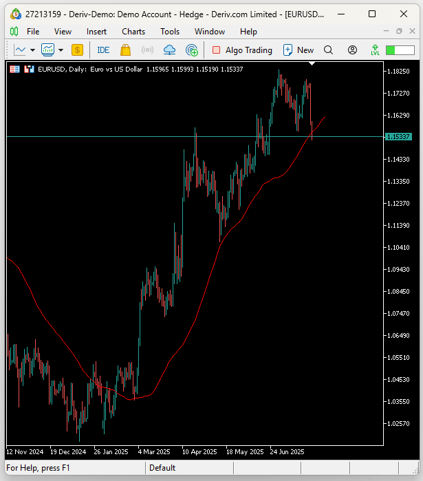
Figure 1: Visualizing our trading strategy in action

Matrix Factorization For Building Linear Classifiers

As in most of our trading applications, we will begin by defining system definitions. In this particular case, we are going to have six inputs that we are keeping track of in our input data matrix X.

//+------------------------------------------------------------------+
//|                                            Linear Regression.mq5 |
//|                                               Gamuchirai Ndawana |
//|                    https://www.mql5.com/en/users/gamuchiraindawa |
//+------------------------------------------------------------------+
#property copyright "Gamuchirai Ndawana"
#property link      "https://www.mql5.com/en/users/gamuchiraindawa"
#property version   "1.00"
//+------------------------------------------------------------------+
//| System constants                                                 |
//+------------------------------------------------------------------+
#define TOTAL_INPUTS 6

Moving on—after defining our system definitions, we now define user inputs that the end user can adjust. In particular, we want our end user to be able to pick the appropriate timeframe and the size of our stop loss.

//+------------------------------------------------------------------+
//| System Inputs                                                    |
//+------------------------------------------------------------------+
int bars = 200;//Number of historical bars to fetch
int horizon = 1;//How far into the future should we forecast
int MA_PERIOD = 50; //Moving average period
ENUM_TIMEFRAMES TIME_FRAME = PERIOD_D1;//User Time Frame
input ENUM_TIMEFRAMES RISK_TIME_FRAME = PERIOD_D1;
input double sl_size = 2;

In addition, we must also include important system libraries that we need, such as the trade library and two custom libraries that I have written for keeping track of time and getting important trading information.

//+------------------------------------------------------------------+
//| Dependencies                                                     |
//+------------------------------------------------------------------+
#include <Trade\Trade.mqh>
#include <VolatilityDoctor\Time\Time.mqh>
#include <VolatilityDoctor\Trade\TradeInfo.mqh>

Moving on, our system is also dependent on us to create important global variables for our exercise. In this particular case, we need global variables to be handlers for our technical indicators. We need global variables to keep track of the input data and the output data as we are receiving it from the market. Also, we need buffers for our technical indicators to retrieve their current values.

//+------------------------------------------------------------------+
//| Global Variables                                                 |
//+------------------------------------------------------------------+
int        ma_close_handler;
double     ma_close[];
Time       *Timer;
TradeInfo  *TradeInformation;
vector     bias,temp,Z1,Z2;
matrix     X,y,prediction,b;
int        time;
CTrade Trade;
int state;
int atr_handler;
double atr[];

When our system is loaded for the first time, we will have a dedicated method called initialize that will be called to initialize all system variables. 

//+------------------------------------------------------------------+
//| Expert initialization function                                   |
//+------------------------------------------------------------------+
int OnInit()
  {
//---
   initialize();
//---
   return(INIT_SUCCEEDED);
  }

When our system is no longer used, we will release the memory that was being consumed by the technical indicators.

//+------------------------------------------------------------------+
//| Expert deinitialization function                                 |
//+------------------------------------------------------------------+
void OnDeinit(const int reason)
  {
//---
   IndicatorRelease(atr_handler);
   IndicatorRelease(ma_close_handler);
  }

Whenever new updated price candles have formed, we will call two dedicated methods. The first method is the setup method, and the last is the findSetup unit. We will discuss these later in detail as we progress.

//+------------------------------------------------------------------+
//| Expert tick function                                             |
//+------------------------------------------------------------------+
void OnTick()
  {
//---
   if(Timer.NewCandle())
     {
      setup();
      find_setup();
     }
  }

When our system is first initialized, we will load new instances of handlers to their appropriate identifiers. So, for example, we will dynamically create a new object for our time library that keeps track of candle formation. We also create a new object for our trade information class. Remember that this class is responsible for keeping track of important details, such as the smallest lot size volume allowed on the current market for trading, and the current ask and bid prices. Additionally, the initialize function is responsible for loading all the default values into our matrices and their associated identifiers.

//+------------------------------------------------------------------+
//| Initialize our system variables                                  |
//+------------------------------------------------------------------+
void initialize(void)
  {
   Timer                   = new Time(Symbol(),TIME_FRAME);
   TradeInformation        = new TradeInfo(Symbol(),TIME_FRAME);
   ma_close_handler        = iMA(Symbol(),TIME_FRAME,MA_PERIOD,0,MODE_SMA,PRICE_CLOSE);
   atr_handler             = iATR(Symbol(),RISK_TIME_FRAME,14);
   bias = vector::Ones(TOTAL_INPUTS);
   Z1 = vector::Ones(TOTAL_INPUTS);
   Z2 = vector::Ones(TOTAL_INPUTS);
   X = matrix::Ones(TOTAL_INPUTS,bars);
   y = matrix::Ones(1,bars);
   time = 0;
   state = 0;
  }

The "find_setup()" function is rather more involved than the other functions that we have considered so far. First, the findSetup function will keep track of the current close price, and then we will copy the current reading from our indicators. Therefore, we will copy the ATR and the moving average readings into their associated buffers. From there, if we have no positions open, we reset the system state. Now we must consider the prediction that we receive from our linear classifier.

Recall that our classifier is modeling two outputs at the same time. The first prediction is the direction that the moving average indicator is expected to follow in the future, while the second prediction will be the gap between the price and the moving average. Therefore, we want these two predictions to be in line with each other. If the moving average indicator is expected to fall, we also want to see price levels falling further beneath it. And if the moving average is expected to rise, we want price levels to rise above it.

These two settings form the basis of our trading strategy. Both predictions should be greater than 0.5 for us to buy. Additionally, both predictions should be less than 0.5 for us to sell. Otherwise, if we already have open positions, then we are simply going to keep track of our position and our linear classifier's expectations. If we are selling, but our model expects the moving average indicator to rise, then we will close our position. And the converse holds true if we are buying.

Otherwise, if all appears to be fine, we will just update our stop loss to a more profitable setting and continue from there.

//+------------------------------------------------------------------+
//| Find a trading setup for our linear classifier model             |
//+------------------------------------------------------------------+
void find_setup(void)
  {
   double c =  iClose(Symbol(),TIME_FRAME,0);
   CopyBuffer(atr_handler,0,0,1,atr);
   CopyBuffer(ma_close_handler,0,0,1,ma_close);

   if(PositionsTotal() == 0)
     {
      state = 0;
      if((prediction[0,0] > 0.5) && (prediction[1,0] > 0.5))
        {
         Trade.Buy(TradeInformation.MinVolume(),Symbol(),TradeInformation.GetAsk(),(TradeInformation.GetBid() - (sl_size * atr[0])),0);
         state = 1;
        }
      if((prediction[0,0] < 0.5) && (prediction[1,0] < 0.5))
        {
         Trade.Sell(TradeInformation.MinVolume(),Symbol(),TradeInformation.GetBid(),(TradeInformation.GetAsk() + (sl_size * atr[0])),0);
         state = -1;
        }
     }

   if(PositionsTotal() > 0)
     {
      if(((state == -1) && (prediction[0,0] > 0.5)) || ((state == 1)&&(prediction[0,0] < 0.5)))
         Trade.PositionClose(Symbol());
      if(PositionSelect(Symbol()))
        {
         double current_sl = PositionGetDouble(POSITION_SL);

         if((state == 1) && ((ma_close[0] - (2 * atr[0]))>current_sl))
           {
            Trade.PositionModify(Symbol(),(ma_close[0] - (2 * atr[0])),0);
           }

         else
            if((state == -1) && ((ma_close[0] + (2 * atr[0]))<current_sl))
              {
               Trade.PositionModify(Symbol(),(ma_close[0] + (2 * atr[0])),0);
              }
        }
     }
  }

We have dedicated methods that we use for fitting our linear classifier. The fit method, as shown below, will fit our data—mapping previous price inputs to the two targets that we are interested in following. Recall that we use the Singular Value Decomposition (SVD) method contained in the OpenBLAS library to quickly factorize our model into a form that allows us to find the optimal coefficients and store them in B.

//+------------------------------------------------------------------+
//| Fir our classification model                                     |
//+------------------------------------------------------------------+
void fit(void)
  {
//--- Fit the model
   matrix OB_U,OB_VT,OB_SIGMA;
   vector OB_S;
   X.SingularValueDecompositionDC(SVDZ_S,OB_S,OB_U,OB_VT);
   OB_SIGMA.Diag(OB_S);
   b = y.MatMul(OB_VT.Transpose().MatMul(OB_SIGMA.Inv()).MatMul(OB_U.Transpose()));
  }

As always, fetching data and storing it is an important part of any machine learning model. We will subtract the mean value and divide by the standard deviation for each of our data entries.

For example, we want to keep track of the open price, the high price, the low price, and the technical indicator values. All these values must be subtracted by the mean and divided by the standard deviation before they are stored into the data matrix X.

Thereafter, after copying and reshaping our Y matrix, we must then store our outputs either as zeros (to indicate the price levels fell) or ones (to indicate the price levels appreciated). This is how we build a classification model.

//+------------------------------------------------------------------+
//| Prepare the data needed for our classifier                       |
//+------------------------------------------------------------------+
void fetch_data(void)
  {
//--- Reshape the matrix
   X = matrix::Ones(TOTAL_INPUTS,bars);

//--- Store the Z-scores
   temp.CopyRates(Symbol(),TIME_FRAME,COPY_RATES_OPEN,horizon,bars);
   Z1[0] = temp.Mean();
   Z2[0] = temp.Std();
   temp = ((temp - Z1[0]) / Z2[0]);
   X.Row(temp,1);

//--- Store the Z-scores
   temp.CopyRates(Symbol(),TIME_FRAME,COPY_RATES_HIGH,horizon,bars);
   Z1[1] = temp.Mean();
   Z2[1] = temp.Std();
   temp = ((temp - Z1[1]) / Z2[1]);
   X.Row(temp,2);

//--- Store the Z-scores
   temp.CopyRates(Symbol(),TIME_FRAME,COPY_RATES_LOW,horizon,bars);
   Z1[2] = temp.Mean();
   Z2[2] = temp.Std();
   temp = ((temp - Z1[2]) / Z2[2]);
   X.Row(temp,3);

//--- Store the Z-scores
   temp.CopyRates(Symbol(),TIME_FRAME,COPY_RATES_CLOSE,horizon,bars);
   Z1[3] = temp.Mean();
   Z2[3] = temp.Std();
   temp = ((temp - Z1[3]) / Z2[3]);
   X.Row(temp,4);

//--- Store the Z-scores
   temp.CopyIndicatorBuffer(ma_close_handler,0,horizon,bars);
   Z1[4] = temp.Mean();
   Z2[4] = temp.Std();
   temp = ((temp - Z1[4]) / Z2[4]);
   X.Row(temp,5);

//--- Reshape the output target
   y.Reshape(2,bars);
   vector temp_2,temp_3,temp_4;

//--- Prepare to label the target accordingly
   temp.CopyRates(Symbol(),TIME_FRAME,COPY_RATES_CLOSE,horizon,bars);
   temp_4.CopyRates(Symbol(),TIME_FRAME,COPY_RATES_CLOSE,0,bars);

   temp_2.CopyRates(Symbol(),TIME_FRAME,COPY_RATES_CLOSE,0,bars);
   temp_3.CopyIndicatorBuffer(ma_close_handler,0,0,bars);

   for(int i=0;i<bars;i++)
     {
      //--- Record if price levels appreciated or depreciated
      if(temp[i] > temp_4[i])
         y[0,i] = 0;
      else
         if(temp[i] < temp_4[i])
            y[0,i] = 1;

      //--- Record if price levels remained above the moving average indicator, or fell beneath it.
      if(temp_2[i] < temp_3[i])
         y[1,i] = 0;
      if(temp_2[i] > temp_3[i])
         y[1,i] = 1;
     }

   Print("Training Input Data: ");
   Print(X);

   Print("Training Target");
   Print(y);
  }

Thereafter, we are now prepared to start getting predictions from our classification model. To simply get a prediction from our classification model, we need the last row in our input data X. Alternatively, we can think of it as the current market reading—the current market conditions. We take those current market conditions and multiply them by the coefficients we learned from historical data, and that will give us a prediction.

//+------------------------------------------------------------------+
//| Obtain a prediction from our classification model                |
//+------------------------------------------------------------------+
void predict(void)
  {
//--- Prepare to get a prediction
//--- Reshape the data
   X = matrix::Ones(TOTAL_INPUTS,1);

//--- Get a prediction
   temp.CopyRates(Symbol(),TIME_FRAME,COPY_RATES_OPEN,0,1);
   temp = ((temp - Z1[0]) / Z2[0]);
   X.Row(temp,1);

   temp.CopyRates(Symbol(),TIME_FRAME,COPY_RATES_HIGH,0,1);
   temp = ((temp - Z1[1]) / Z2[1]);
   X.Row(temp,2);

   temp.CopyRates(Symbol(),TIME_FRAME,COPY_RATES_LOW,0,1);
   temp = ((temp - Z1[2]) / Z2[2]);
   X.Row(temp,3);

   temp.CopyRates(Symbol(),TIME_FRAME,COPY_RATES_CLOSE,0,1);
   temp = ((temp - Z1[3]) / Z2[3]);
   X.Row(temp,4);

   temp.CopyIndicatorBuffer(ma_close_handler,0,0,1);
   temp = ((temp - Z1[4]) / Z2[4]);
   X.Row(temp,5);

   Print("Prediction Inputs: ");
   Print(X);

//--- Get a prediction
   prediction = b.MatMul(X);
   Print("Prediction");
   Print(prediction);
  }

However, calling each of these methods one by one can be cumbersome. Therefore, we have designed a dedicated setup method that will call each of these three methods in the order that we need them. First, we will fetch the data. Then we will fit our model onto the data. And lastly, we will get a prediction.

This simple setup method allows us to perform all three steps—always in the right order.

//+------------------------------------------------------------------+
//| Obtain a prediction from our model                               |
//+------------------------------------------------------------------+
void setup(void)
  {
   fetch_data();
   fit();
   predict();
  }
//+------------------------------------------------------------------+

Lastly, we must unify the system definitions that we made at the beginning of our application.

#undef TOTAL_INPUTS

Our backtest will begin in January 2020 and run for five years on the daily timeframe, up until 2025. We will be testing our application on the EURUSD symbol.

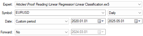
Figure 2: Selecting our backtest and optimization days

Additionally, for the best settings possible, we always use random delay settings to ensure that the conditions we test our application in will match the real market environments that we are expecting to see in the future.

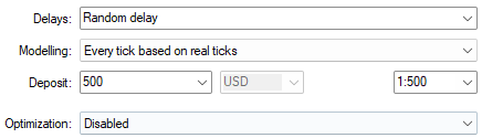
Figure 3: Selecting our backtest conditions is also important

I took a screenshot of the performance of our application during the backtest. As we can see, the application is showing us the prediction inputs that it was given. Recall that the first input is always one to represent the intercept. But really, our attention is being paid mostly to the actual predictions being given by our model.

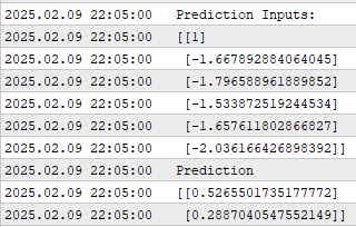
Figure 4: The output obtained from running our linear classifier algorithm

As we can see, our model is giving us two predictions, as we stated before. The first prediction is associated with the change in the moving average’s position in the future, while the second prediction is associated with the change between price relative to the moving average. And recall that we want both of these changes to be in a uniform direction.

We can also observe the equity curve produced by our trading strategy. As we can see, the equity curve has an upward trend over time, although it is not entirely stable.

Additionally, the reader should be aware that there are two lines being illustrated in this curve. The blue line is our balance over time, and the green line is the equity in the account over time. So, as we can see, there are many instances where we observe the equity—the green line—spiking above the blue line.

From my experience as the writer, this represents missed profits or signals in our trading strategy that we are still failing to pick up. This signal is getting past our trading strategy, and we are not capitalizing on those profits. This suggests that there is still room for improvement in our strategy.

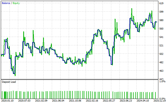
Figure 5: Our equity curve is signaling to us that there is still some signal we are failing to learn.

Lastly, we can consider the detailed statistics of our performance over time. And as we can see, on average, our average profitable trade is greater than our average losing trade. The largest profit we made following our strategy is also greater than the largest loss that we made, which is encouraging to see.

However, when we look at the percentage of profitable trades, we see that we have 43% profitable trades, which is less than half. This reinforces what I brought to the reader’s attention when we looked at the equity curve and saw those spikes of missed equity that our system failed to realize.

This just really enforces our belief that the system can be improved further—that there is information we are still not picking up. Even though this is a strong start, there is more signal that we can uncover and learn.

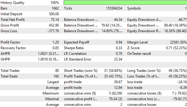
Figure 6: The detailed statistics of our performance support our earlier deductions that the system has room for improvement

Conclusion 

In conclusion, this article has demonstrated to the reader the multiple applications of matrix factorization that we, as algorithmic traders, can take advantage of in our MQL5 applications. When we first brought up matrix factorization, we looked at it as a tool that can be used for regression. Now, we are looking at it as a tool that can be used for classification.

But I make the reader only one promise—that there is still yet a lot more for us to cover. These are just the basics. These are, in my opinion as the writer, the easy applications that quickly show us the value of matrix factorization. If you have been following this series of articles, then you leave now knowing how to build a regression model using matrix factorization, or a classifier model, or a combination of both—models that are not just limited to one prediction at a time but that can predict multiple targets at once.

And yet, I promise you, the reader, that there are still many more benefits of matrix factorization that we have yet to cover. But before we can start to explore those benefits, we must first master the basics. Additionally, you have seen how easy it is—thanks to the dedicated functions available to us in the MQL5 API. You have seen how easy it is to include these powerful matrix methods into your trading applications.