Rebuy algorithm: Multicurrency trading simulation

Contents

• Introduction
• Explaining the need for trading simulation
• Mathematical model of price simulation using discretization logic
• Model testing
• Test EA
• Conclusion

Introduction

In the previous article I showed you a lot of useful features that you probably did not know, but the most interesting thing is ahead - research or trading simulation. Sometimes a strategy tester is not enough. Although this is a very convenient tool for getting to know the market, but this is only the first step. If you carefully read the previous article, then you most likely know the reason already.

Explaining the need for trading simulation

The reason for trading simulation lies directly in the fact that the amount of historical data of any trading instruments is limited. This issue can be seen only if you understand the material I provided in the previous article or in some other alternative way.  

The essence of the problem is that a simple history of quotes is not always sufficient, because this history is formed at the intersection of many random and non-random world events, and there are countless scenarios for the event to unfold. Currently, I am trying to describe things as simple as possible, but if we move on to the language of probability theory and at the same time use the achievements of the previous article, we understand that the history of quotes of all instruments known to us could develop differently.

This fact is obvious, if you watched the movie "Back to the Future". It has a lot of blunders and funny inconsistencies from the scientific point of view, but, nevertheless, this film conveys the main idea of the message provided here. The essence of the message is that one version of events unfolding is not enough for us, and we should consider their maximum number. History gives us only one version, and its size may sometimes be insufficient for an objective assessment. For example, not so long ago, many brokers have obtained some of the most popular crypto symbols. This is very good in terms of the possibility of testing and trading these symbols. But the downside is that there is not enough historical data to develop sustainable trading systems for EAs that work on bars.

The simulation will allow creating artificial instruments and generate their quotes every time in a completely different way. This will provide us with the widest possible framework for studying the mathematical rebuy model and other important mathematical principles I talked about in the previous article. Another important advantage is that we will be able to simulate an unlimited number of independent instruments for parallel trading. Ultimately, we no longer have a limitation on the duration of testing and the number of independently traded instruments. Of course, these will not be real quotes, but they will not differ in any way from real ones in terms of pricing laws.

Mathematical model of price simulation using discretization logic

In the context of our task, the use of the "arbitrary discretization" approach is more than enough, because strong discretization will only increase the efficiency of our algorithm, if only because such systems automatically resist spreads more effectively. However, I have built an algorithm that allows simulation of ticks as well. After all, a tick is the smallest timeframe. The time between tick arrivals is very different, but if you calculate the average time between ticks, then you can imitate ticks as a first approximation.

By a bar in this case, we mean a fixed period of time, which is convenient for us to perceive from a visual point of view. But this is convenient only because you were told that it is convenient, and you cannot get away from it, because all trading terminals are tailored specifically for this paradigm. However, this is far from the best way to discretize pricing. I think, many of you are familiar with "renko". This approach to price discretization is intended only for one thing - to get away from time. The value of this approach can be completely different for different approaches and traders. However, I use this example only to show one of the alternative ways to discretize price series. This example, in my understanding, should tell you that in the context of our task we will use a completely different and unfamiliar discretization logic, but it will allow us to model pricing very simply and efficiently without excessive computational costs.

For the correct construction of an efficient and economical paradigm in terms of computing power, have a look at the following image:

The image shows a couple of possible scenarios for price rollbacks. These two rollbacks for me denote arbitrary two points that can be chosen in absolutely any way, and the choice method is of no importance. The important thing is that we can arbitrarily choose any point that can be considered as a likely reversal point.

The word "probable" should immediately tell every mathematician that at a given point there is some probability of some desired event. In our case, we can say that a given event can be arbitrary. The rollback event is characterized by the upper and lower boundaries of the price increment. The probability of this event can be calculated the following way:

Here is the probability of reaching the upper bound and the equation this formula is derived from. The equation characterizes the mathematical expectation of the price increment if there is no predictive moment. The lack of predictive moment translates into zero expectation, but in our simulation I want to be able to adjust the predictive moment parameters so that we can conveniently boost or weaken the flat characteristics of our simulated pricing. Ultimately, you will see how this affects the rebuy algorithm, and you will get a working mathematical model for diversified trading using the rebuy algorithm. But first I want to give you the full math behind all this.

Currently, we can see that all these equations are beautiful and seemingly useful, but so far there is no convenient algorithm for adjusting the flatness (rollback) of the instrument. To develop such an algorithm, we need to enter the following values:

The first value is actually the average "alpha" value. We can also call it the mathematical expectation of the price rollback value after an arbitrary downward movement. The second value is the mathematical expectation of the rollback percentage expressed as a relative value to its previous movement. The essence of these quantities is the same with the only exception:

Here I am just showing you how these quantities are related and how they are calculated. In our model, we will regulate the average rollback setting its average percentage and we will reverse the logic using it to determine the average price rollback. You must admit that the average rollback percentage is very convenient as a regulatory value for the market flatness parameter. If this percentage is set to zero, then we actually require random pricing (this is just an example). The only thing I want to note is that all price drawdowns are considered relative to the "theta" point. I hope you will forgive me the liberties in my notation, because this material is completely mine, and there is not a drop of someone else's work here. These equations are needed to understand what I will do next.

Another important characteristic of any pricing is volatility (price change rate). This parameter is associated with time, and we must come up with some extremely convenient way to set this value. This should allow us to easily and effectively control the rate of pricing, as well as correctly calculate the timing of trading cycles. Currently, all this might seem too complicated, but it will be much clearer when I get down to practice and start showing you how it works. Let's deal with volatility first.

In the classical interpretation, volatility is a little different, rather, the degree of possible relative price movement from a minimum to a maximum and vice versa, from a maximum to a minimum. This is a very inconvenient way to set the price movement rate. There is a much more convenient way, which involves measuring the average price movement over a fixed period of time. We have such segments. They are called bars. In fact, we have the law of distribution of a random variable of the price change modulus per bar. The larger this value, the greater the price volatility (change rate). We enter the following settings:

As to whether the random distribution of the "S" value should be simulated, I can say that it is not necessary. The only thing you need to know is that the actual pricing will be different from the method we will use in the mathematical model. I propose to fix the "S" value at the level of its average value. Since the time of each step is already fixed, we get both the size of the step and its duration in time. This will allow us to subsequently evaluate the annual profitability of the trading system, as well as measure the average time of the trading cycle. Now let's have a look at the following picture to move forward:

Since we will have to simulate pricing for each step, it is obvious that the step can be either down or up. If we set an equiprobable step in both directions, then we get random pricing. This means that in order to regulate the flatness, we should change these step probabilities. This will be the provision of some kind of "gravity" to the starting point of the price, from which the price began to move up or down. In our case, we will need to realize the following:  

In this case, to simplify the model, I assumed that the chosen average price reversal requires exactly the same time that was spent on the previous price rise or fall. The purpose of these calculations is to determine the instantaneous expectation for a single step, in order to calculate the probability that the step will occur upwards. With this probability, the simulation of the new step is adjusted. This value is recalculated after each step for each individual trading instrument.

Here is a very important point: if we describe each instrument separately, then we will have to create an array with data on the average price change for each of them. But within the framework of my task, all instruments are equal, and therefore it is possible to introduce a general and more convenient characteristic for describing a step in the form of an average percentage of price change:

The advantage of this characteristic is that it is invariant relative to to any current price. Moreover, if we consider ideal instruments, then it does not matter at what price the simulation starts, because this will not affect the profit or loss during testing. After we understand this, then we can safely start parallel trading for our rebuy algorithm from a price, say, equal to 1. After determining this value, it is already possible to calculate the step value itself:

Now, knowing the step, we can state that we have collected all the necessary data to calculate the probability that there will be a step upwards. To do this, we use our original formula for the mathematical expectation of a step with some substitutions:

After this substitution, we can solve this equation for the probability of an upward step and, finally, get the missing probability:

The only thing worth noting is that these equations are valid for the case when the simulation price falls below the starting point. But what to do when the price went upwards? Everything is very simple. We just need to consider the mirror chart. This can be done because we are considering perfect instruments. If we imagine that the price chart can be described by a certain expression "P = P(t)", then the reversal of the instrument will look like this:

This reversal will keep the equations working for the situation when the price has gone above the starting point. The only thing we need to understand is that all quantities in our expressions that are calculated using prices (for example, deltas) must use the already converted price raised to the minus first power.

Let's now build a trading model. I made it one-way as it was originally intended for spot trading of cryptocurrencies. However, this trading model is also suitable for forex currency pairs. The thing is that if the model works, for example, only in the case of a rebuy, then it will work equally well for a resell. The only thing is that during the test we will skip the upper half-waves and work only on the lower ones. To manage the trading model, I entered the following characteristics:

The starting buy starts from the price "1-Step Percent/100", and the rebuy step will be equal to "Step Percent/100". In fact, there should still be a multiplication by the starting price, but since we take this price equal to one, the calculation of the step is greatly simplified. In addition, the possibility of recurrent step increase has been introduced. For example, we can either increase each next rebuy step relative to the previous one by N times, or decrease it in the same way. All this depends on the value of the corresponding coefficient. The rebuy step is measured in the lower currency of the instrument (not the base one). This rule also works for cryptocurrencies.

To simplify the model, it is assumed that the applied trading instruments in this case are approximately as follows: EURUSD, GBPUSD, NZDUSD and so on, that is, the lower currency of the traded instrument for all traded instruments must be the same. This simplifies an already very complex model, but it is quite sufficient both to test the mathematical principles from the last article and to optimize rebuy algorithms. The spread in our case is taken into account in the form of a commission, which is the same thing. In general, the parameters are sufficient for the mathematical model prototype. Let's take a look at the rebuy process:

We will use the first option (with the green return motion). This is actually buying the base currency and then selling it at the blue dot. With this approach, any completed trading cycle will be profitable. The same applies to the selling cycle with a red return movement, but we will skip them, as I said, in order for the model to be as multifunctional as possible and suitable for both trading on the forex market and spot trading on cryptocurrency exchanges.

The model is made in such a way that the trading leverage does not play a role. I think that I have given you enough theoretical information so that you can better understand the practical part, and it may help someone to build their own model using my achievements.

Model testing

Let's start our testing with different variations of quotes generation. To visually show you the difference in generating quotes, let's first set the model to the following position:

With this setting, we will achieve random pricing. Let's look at a couple of generated quotes from this point of view:

This is a chart from a mathematical model, which shows two quotes randomly taken from the deck and another additional curve, which has the largest deviation from the starting price. In the mathematical model, it is possible to set the required number of instruments to be simulated in parallel, and it is natural that there are a lot of them, and there will always be one that is the least symmetrical and most volatile. But I hope you understand that this is only the result of probabilistic processes. Now let's put the parameter in a different position:

As you might have already understood, this step creates a return gravity of the price to the starting point. The result is as follows:

Notice the difference between the previous and the current image. Here we have already forced the flat adjustment into the desired direction. We can see that the curves are strongly pressed against the starting price - the same thing happened with the most volatile quote colored in black. Both examples simulate exactly one thousand steps for each tool. Later I will increase these numbers and tinker with them to understand how it all works and what parameters are exactly affected.

Now it is necessary to determine what parameters are to be used to test artificial trading ans how it should be tested. Let's quickly recall the questions that I answered in the previous article. In a simpler and more understandable way, they sounded as follows:

1. Condition of profitability of trading systems with rebuy.
2. Does the profit line tend to a perfect straight line when trading endlessly for ideal trading instruments?
3. Does the profit line tend to a perfect straight line as the number of instruments increases to infinity with a fixed time period of trading?

Let's find out the condition of profitability. To do this, let's first conduct parallel trading using random pricing and look at the result. It will look approximately as follows:

In different generations, either profitable or unprofitable curves were obtained. It is not yet clear, but the confirmation of the futility of rebuys in case of random pricing may be an extreme increase in the number of instruments traded in parallel. Let's see what happens if we increase their number to, say, a hundred, and at the same time increase the number of simulation steps for each tool to 10,000:

As you can see, neither the increase in the number of instruments traded in parallel, nor the increase in the duration of testing had any visible effect. Most probably, this confirms the mathematically proven fact from the previous article that any trading system, including the rebuy algorithm, drains the account in case of completely random pricing and without a predictive moment,. At this stage, I consider the point 1 theoretically and practically proven. Let's now move on to the second point and set the following setting:

According to my tests, the return gravity turned out to be quite sufficient for the possibility of a visual assessment of the effect for any reader. Of course, we can set a lower percentage, but the effect will not be so pronounced. I reset the number of simulation steps to the original value of a thousand steps. Now let's look at the result:

I think it will not be difficult to understand that this graph, among other things, is an addition to the proof of the previous paragraph, but, at the same time, it is also a starting point for the proof of the next subparagraph. The next thing in my plan is increasing the duration of all test segments without changing any other parameters. For clarity, I increased the number of simulation steps for each tool fifty times - from 1000 to 50,000. This is a fairly large increase, but this is the only way to visually feel this effect without multiple tests and averaging the results. Let's have a look at the result:

As we can see, the curve has become much smoother and approaches a straight line, which means that the second principle of increasing the linearity factor (graph beauty) with increasing test duration works exactly as predicted. Of course, this is true only with the assumption that it is known that the chosen strategy is profitable. At this stage, I consider the second subparagraph to be theoretically and practically proven.

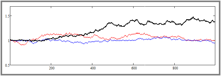
Now let's return the number of simulation steps to the initial level of a thousand steps, and, conversely, increase the number of instruments traded in parallel by ten times, up to the value of 1000. According to the legend, we should get a visible increase in the graph beauty. Let's see if that is true:

As we can see, this hypothesis has been confirmed, and the effect is extremely pronounced. At this stage, I believe that all three hypotheses are theoretically and practically proven. The results are as follows:

1. The condition for the profitability of any trading system is the presence of a predictive moment.
2. With an increase in the duration of trading or backtesting, any curve of a profitable trading system becomes more beautiful and straight (without auto lot) + [provided that the point 1 is fulfilled].
3. With an increase in the number of traded currency pairs for one multi-currency trading system or an increase in the number of simultaneously traded systems, the profitability curve of the trading system becomes more beautiful and straight + [provided that the point 1 for each of these systems is fulfilled].

Test EA

We have figured out how to use trading systems correctly, including the rebuy algorithm, in order to make money as efficiently and safely as possible with both automatic and manual trading. The calculation of money management and other various situations for the correct combination of trading systems deserve a separate article I am going to write a little later.

I have added this section so that you can clearly see the fact that the rebuy algorithm is a working strategy. To do this, I created a test EA that repeats our mathematical model, with the only difference that it also processes the upper half-waves (sell trading cycles). I found some settings that prove the possibility of creating a similar trading system for MetaTrader 5. Here is one of them:

Testing was carried out in the period from 2009 to 2023 using parallel testing of all "28" currency pairs similar to our mathematical model. I used the multibot template I described in one of the previous articles to construct the test algorithm. Of course, the profit curve is far from ideal, and the initial deposit for such trading should be huge, but, nevertheless, my task in this article is not to give you a ready-made robot, but to demonstrate proximity to the mathematical model. The most important thing that you should understand is that with certain modifications, this algorithm will be much safer, more efficient and more viable. I suggest that you discover the essence of the improvements yourself. I think that it will be fair, given that I show things that are usually hidden.

The Expert Advisor, along with the set, as well as the mathematical model itself, are attached to the article as a file, and you can, if you wish, study their structure in more detail and, perhaps, develop the idea much further. In fact, there is much more use in my mathematical model than I have described here. It calculates many important trading characteristics thanks to its own set of output parameters after the backtest. Of course, its functionality is very limited, but it is sufficient for the proof and approximate estimates.

Conclusion

In this article, I have completed the practical part of proving that the principle of diversification works and should be used. Most importantly, in combination with previous article, I have proven both theoretically and practically many important things allowing you at the very least to increase the efficiency of your trading. In addition, the survivability of the rebuy algorithm for more than a decade has been proven with the help of the created EA.

Considering that, we have got confirmation of the wave theory of pricing, or the market flatness. I advise you to pay attention to this article as an additional confirmation. In it, the author pays maximum attention to exactly the same algorithm as I described in my article. From there, you can get additional knowledge on how to use these effects to improve my test EA or develop your own.