
Deep Neural Networks (Part I). Preparing Data
DNN are widely used and intensely developed in many areas. The most common examples of everyday use of neural networks are speech and image recognition and automatic translation from one language into another. DNN are also used in trading. Given the fast development of algorithmic trading, in-depth studying of DNN seems to be useful.
Lately, developers have come up with many new ideas, methods and approaches to the use of DNN and proved them experimentally. This series of articles will consider the state and the main directions of the development of DNN. A lot of space will be dedicated to testing various ideas and methods using practical experiments alongside qualitative characteristics of DNN. In our work we will be using only multilayer fully connected networks.
The articles will have four focus areas:
- Preparation, evaluation and amplification of the entry data by various transformations.
- New capabilities of the darch package (v.0.12). Flexibility and extended functionality.
- The use of prediction result amplification (optimization of hyperparameters of DNN and ensembles of neural networks).
- Graphical capabilities for controlling the work of an Expert Advisor both during learning and work.
This article will consider preparing data received in the trading terminal for use in the neural network.
Contents
- Introduction. The R language
- 1. Creating initial (raw) data
- 2. Exploratory data analysis
- 3. Preparing Data
- Application
- Links
Introduction
Development, training and testing of a deep neural network are done in stages that have a strict sequence. Similar to any model of machine learning, the process of creating a DNN can be split into two unequal parts:
- preparing input and output data for experiments;
- creating, training, testing and optimizing parameters of the DNN.
The first stage takes a bigger part of the project time - about 70%. The work of a DNN largely depends on the success of the this stage. After all, garbage in - garbage out. This is why we will describe the sequence of actions at this stage in detail.
To repeat the experiments, you will need to install MRO 3.4.0 and Rstudio. Instructions for installing this software can be easily found on the internet. Files attached to this article contain this information too so we are not going to consider it in detail.
The R language
Let us recall some important things about R. This is a programming language and environment for statistical computing and graphics. It was developed in 1996 by New Zealand scientists Ross Ihaka and Robert Gentleman at the University of Auckland. R is a GNU project, that is open source software. The approach to using open source software goes down to the following principles (freedoms):
- the freedom to launch programs for any purpose (freedom 0);
- the freedom to study how the program works and adapt it to the programmer's needs (freedom 1);
- the freedom to distribute copies so you can help your neighbor (freedom 2);
- the freedom to improve the program and distribute the modified version to benefit the whole community with the change.
Today R is being improved and developed mainly by "R Development Core Team" and R Consortium founded last year. The list of the members of the consortium (IBM, Microsoft, Rstudio, Google, Mango, Oracle and others) indicates good support, significant interest and good prospects of the language.
Advantages of R:
- Today, R is the standard in statistical computing.
- It is supported and developed by the world's scientific community.
- A wide set of packages concerning all advanced direction in data mining. It must be mentioned that the time between a publication of a new idea by scientists and the implementation of this idea in R is no more than two weeks.
- And, last but not least, it is absolutely free.
1. Creating initial (raw) data
"All of the previous, current and future price movements are in the price itself"
There are many methods (packages) designed for preliminary preparation, evaluation and choosing of the predictors. The review of these methods can be found in [1]. Their variety is explained by the diversity of real world data. The data type in use will define the methods of exploring and processing.
We are exploring financial data. These are hierarchical, regular timeseries which are infinite and can be easily extracted. The base row is the OHLCV quotes for the instrument on the specific timeframe.
All other timeseries come from this base row:
- nonparametric. For example, x^2, sqrt(abs(x)), x^3, -x^2 etc.
- functional nonparametric. For example, sin(2*n*x), ln(abs(x)), log(Pr(t)/Pr(t-1)) etc.
- parametric. Here belongs a number of various indicators, which are mainly used as predictors. They can be both oscillators and different sorts of filter.
Either indicators generating signals (factors) or a sequence of conditional statements producing a signal can be used as the goal variable.
1.1. Quotes
The OHLC quotes, Volume and time we get from the terminal as the (o, h, l, cl, v, d) vectors. We need to write a function that will join vectors received from the terminal in dataFrame. For that, we will change the format of the start time of the bar to the POSIXct format.
#---pr.OHLCV-------------------
pr.OHLCV <- function(d, o,  h,  l,  cl, v){
# (d, o,  h,  l,  cl, v)- vector
  require('magrittr')
  require('dplyr')
  require('anytime')
  price <- cbind(Data = rev(d),
                 Open = rev(o), High = rev(h),
                 Low = rev(l), Close = rev(cl),
                 Vol = rev(v)) %>% as.tibble()
  price$Data %<>% anytime(., tz = "CET")
  return(price)
}
As the quote vectors have been loaded in the environment env, let us calculate the dataFrame pr and clear the environment env from unused variables:
evalq({pr <- pr.OHLCV(Data, Open, High, Low, Close, Volume)
       rm(list = c("Data", "Open", "High", "Low", "Close", "Volume"))
       },
env)
We want to see how this dataFrame looks at the beginning:
> head(env$pr)
# A tibble: 6 x 6
                 Data    Open    High     Low   Close
               <dttm>   <dbl>   <dbl>   <dbl>   <dbl>
1 2017-01-10 11:00:00 122.758 122.893 122.746 122.859
2 2017-01-10 11:15:00 122.860 122.924 122.818 122.848
3 2017-01-10 11:30:00 122.850 122.856 122.705 122.720
4 2017-01-10 11:45:00 122.721 122.737 122.654 122.693
5 2017-01-10 12:00:00 122.692 122.850 122.692 122.818
6 2017-01-10 12:15:00 122.820 122.937 122.785 122.920
# ... with 1 more variables: Vol <dbl>
and at the end:
> tail(env$pr)
# A tibble: 6 x 6
                 Data    Open    High     Low   Close
               <dttm>   <dbl>   <dbl>   <dbl>   <dbl>
1 2017-05-05 20:30:00 123.795 123.895 123.780 123.888
2 2017-05-05 20:45:00 123.889 123.893 123.813 123.831
3 2017-05-05 21:00:00 123.833 123.934 123.825 123.916
4 2017-05-05 21:15:00 123.914 123.938 123.851 123.858
5 2017-05-05 21:30:00 123.859 123.864 123.781 123.781
6 2017-05-05 21:45:00 123.779 123.864 123.781 123.781
# ... with 1 more variables: Vol <dbl>
So, there are 8000 bars with the start date 10.01.2017 and the end date 05.05.2017. Let us add derivatives of the price to the dataframe pr — Medium Price, Typical Price and Weighted Close
evalq(pr %<>% mutate(.,
                  Med = (High + Low)/2,
                  Typ = (High + Low + Close)/3,
                  Wg  = (High + Low + 2 * Close)/4,
                  #CO  = Close - Open,
                  #HO  = High - Open,
                  #LO  = Low - Open,
                  dH  = c(NA, diff(High)),
                  dL  = c(NA, diff(Low))
                  ),
      env)
1.2. Predictors
We are going to work with a set of simplified predictors. Digital filters FATL, SATL, RFTL, RSTL will play that role. They are described in detail in the article by V. Kravchuk "New Adaptive Method of Following the Tendency and Market Cycles", which can be found in the files attached to this article (see the chapter "New Tools of Technical Analysis and their Interpretation"). Here I will just list them.
- FATL (Fast Adaptive Trend Line);
- SATL (Slow Adaptive Trend Line);
- RFTL (Reference Fast Trend Line);
- RSTL (Reference Slow Trend Line).
The rate of change of FATL and SATL can be monitored using the FTLM (Fast Trend Line Momentum) and STLM (Slow Trend Line Momentum) indicators.
There are two oscillators among the technical tools that we will need - indices RBCI and PCCI. The RBCI (Range Bound Channel Index) index is a bandwidth limited channel index which is calculated by means of a channel filter. The filter removes low frequency trend and low frequency noise. The PCCI (Perfect Commodity Channel Index) index is a perfect commodity channel index.
The function calculating digital filters FATL, SATL, RFTL, RSTL looks as follows:
#-----DigFiltr-------------------------
DigFiltr <- function(X, type = 1){
# X - vector
  require(rowr)
  fatl <- c( +0.4360409450, +0.3658689069, +0.2460452079, +0.1104506886, -0.0054034585,
             -0.0760367731, -0.0933058722, -0.0670110374, -0.0190795053, +0.0259609206,
             +0.0502044896, +0.0477818607, +0.0249252327, -0.0047706151, -0.0272432537,
             -0.0338917071, -0.0244141482, -0.0055774838, +0.0128149838, +0.0226522218,
             +0.0208778257, +0.0100299086, -0.0036771622, -0.0136744850, -0.0160483392,
             -0.0108597376, -0.0016060704, +0.0069480557, +0.0110573605, +0.0095711419,
             +0.0040444064, -0.0023824623, -0.0067093714, -0.0072003400, -0.0047717710,
             0.0005541115, 0.0007860160, 0.0130129076, 0.0040364019 )
  rftl <- c(-0.0025097319, +0.0513007762 , +0.1142800493 , +0.1699342860 , +0.2025269304 ,
            +0.2025269304, +0.1699342860 , +0.1142800493 , +0.0513007762 , -0.0025097319 ,
            -0.0353166244, -0.0433375629 , -0.0311244617 , -0.0088618137 , +0.0120580088 ,
            +0.0233183633, +0.0221931304 , +0.0115769653 , -0.0022157966 , -0.0126536111 ,
            -0.0157416029, -0.0113395830 , -0.0025905610 , +0.0059521459 , +0.0105212252 ,
            +0.0096970755, +0.0046585685 , -0.0017079230 , -0.0063513565 , -0.0074539350 ,
            -0.0050439973, -0.0007459678 , +0.0032271474 , +0.0051357867 , +0.0044454862 ,
            +0.0018784961, -0.0011065767 , -0.0031162862 , -0.0033443253 , -0.0022163335 ,
            +0.0002573669, +0.0003650790 , +0.0060440751 , +0.0018747783)
  satl <- c(+0.0982862174, +0.0975682269 , +0.0961401078 , +0.0940230544, +0.0912437090 ,
            +0.0878391006, +0.0838544303 , +0.0793406350 ,+0.0743569346 ,+0.0689666682 ,
            +0.0632381578 ,+0.0572428925 , +0.0510534242,+0.0447468229, +0.0383959950,
            +0.0320735368, +0.0258537721 ,+0.0198005183 , +0.0139807863,+0.0084512448,
            +0.0032639979, -0.0015350359, -0.0059060082 ,-0.0098190256 , -0.0132507215,
            -0.0161875265, -0.0186164872, -0.0205446727, -0.0219739146 ,-0.0229204861 ,
            -0.0234080863,-0.0234566315, -0.0231017777, -0.0223796900, -0.0213300463 ,-0.0199924534 ,
            -0.0184126992,-0.0166377699, -0.0147139428, -0.0126796776, -0.0105938331 ,-0.0084736770 ,
            -0.0063841850,-0.0043466731, -0.0023956944, -0.0005535180, +0.0011421469 ,+0.0026845693 ,
            +0.0040471369,+0.0052380201, +0.0062194591, +0.0070340085, +0.0076266453 ,+0.0080376628 ,
            +0.0083037666,+0.0083694798, +0.0082901022, +0.0080741359, +0.0077543820 ,+0.0073260526 ,
            +0.0068163569,+0.0062325477, +0.0056078229, +0.0049516078, +0.0161380976 )
  rstl <- c(-0.0074151919,-0.0060698985,-0.0044979052,-0.0027054278,-0.0007031702,+0.0014951741,
            +0.0038713513,+0.0064043271,+0.0090702334,+0.0118431116,+0.0146922652,+0.0175884606,
            +0.0204976517,+0.0233865835,+0.0262218588,+0.0289681736,+0.0315922931,+0.0340614696,
            +0.0363444061,+0.0384120882,+0.0402373884,+0.0417969735,+0.0430701377,+0.0440399188,
            +0.0446941124,+0.0450230100,+0.0450230100,+0.0446941124,+0.0440399188,+0.0430701377,
            +0.0417969735,+0.0402373884,+0.0384120882,+0.0363444061,+0.0340614696,+0.0315922931,
            +0.0289681736,+0.0262218588,+0.0233865835,+0.0204976517,+0.0175884606,+0.0146922652,
            +0.0118431116,+0.0090702334,+0.0064043271,+0.0038713513,+0.0014951741,-0.0007031702,
            -0.0027054278,-0.0044979052,-0.0060698985,-0.0074151919,-0.0085278517,-0.0094111161,
            -0.0100658241,-0.0104994302,-0.0107227904,-0.0107450280,-0.0105824763,-0.0102517019,
            -0.0097708805,-0.0091581551,-0.0084345004,-0.0076214397,-0.0067401718,-0.0058083144,
            -0.0048528295,-0.0038816271,-0.0029244713,-0.0019911267,-0.0010974211,-0.0002535559,
            +0.0005231953,+0.0012297491,+0.0018539149,+0.0023994354,+0.0028490136,+0.0032221429,
            +0.0034936183,+0.0036818974,+0.0038037944,+0.0038338964,+0.0037975350,+0.0036986051,
            +0.0035521320,+0.0033559226,+0.0031224409,+0.0028550092,+0.0025688349,+0.0022682355,
            +0.0073925495)
  if (type == 1) {k = fatl}
  if (type == 2) {k = rftl}
  if (type == 3) {k = satl}
  if (type == 4) {k = rstl}
  n <- length(k)
  m <- length(X)
  k <- rev(k)
  f <- rowr::rollApply(data = X,
                       fun = function(x) {sum(x * k)},
                       window = n, minimum = n, align = "right")
  while (length(f) < m) { f <- c(NA,f)}
  return(f)
}
After they have been calculated, add them to the dataframe pr
evalq(pr %<>% mutate(.,
                   fatl = DigFiltr(Close, 1),
                   rftl = DigFiltr(Close, 2),
                   satl = DigFiltr(Close, 3),
                   rstl = DigFiltr(Close, 4)
                   ),
      env)
Add oscillators FTLM, STLM, RBCI, PCCI, their first differences and the first differences of the digital filters to the dataframe pr:
evalq(pr %<>% mutate(.,
                     ftlm = fatl - rftl,
                     rbci = fatl - satl,
                     stlm = satl - rstl,
                     pcci = Close - fatl,
                     v.fatl = c(NA, diff(fatl)),
                     v.rftl = c(NA, diff(rftl)),
                     v.satl = c(NA, diff(satl)),
                     v.rstl = c(NA, diff(rstl)*10)
                     ),
      env)
evalq(pr %<>% mutate(.,
                     v.ftlm = c(NA, diff(ftlm)),
                     v.stlm = c(NA, diff(stlm)),
                     v.rbci = c(NA, diff(rbci)),
                     v.pcci = c(NA, diff(pcci))
                    ),
      env)
1.3. Goal variable
ZigZag() will be used as the indicator generating the goal variable.
The function for its calculation will receive the timeseries and two parameters: a minimal length of a bend (int or double) and the price type for calculation (Close, Med, Typ, Wd, with (High, Low) ).
#------ZZ-----------------------------------
par <- c(25, 5)
ZZ <- function(x, par) {
# x - vector
  require(TTR)
  require(magrittr)
  ch = par[1]
  mode = par[2]
  if (ch > 1) ch <- ch/(10 ^ (Dig - 1))
  switch(mode, xx <- x$Close,
         xx <- x$Med, xx <- x$Typ,
         xx <- x$Wd, xx <- x %>% select(High,Low))
  zz <- ZigZag(xx, change = ch, percent = F,
               retrace = F, lastExtreme = T)
  n <- 1:length(zz)
  for (i in n) { if (is.na(zz[i])) zz[i] = zz[i - 1]}
  return(zz)
}
Calculate ZigZag, the first difference, the sign of the first difference and add them to the dataframe pr:
evalq(pr %<>% cbind(., zigz = ZZ(., par = par)), env)
evalq(pr %<>% cbind(., dz = diff(pr$zigz) %>% c(NA, .)), env)
evalq(pr %<>% cbind(., sig = sign(pr$dz)), env)
1.4.Initial data set
Let us sum up what data we should have as a result of calculations.
We received from the terminal the OHLCV vectors and a temporary mark of the beginning of the bar on the M15 timeframe for EURJPY. These data formed the pr dataframe. Variables FATL, SATL, RFTL, RSTL, FTLM, STLM, RBCI, PCCI and their first differences were added to this dataframe. ZigZag with a minimal leverage of 25 points (4 decimal places), its first difference and the sign of the first difference (-1,1), which will be used as a signal, were added to the dataframe too.
All these data were loaded not into the global environment but into a new child environment env, where all the calculations will be carried out. This division will allow using data sets from different symbols or timeframes without name conflicts during calculation.
The structure of the total dataframe pr is shown below. Variables, required for the following calculations can be easily extracted from this.
str(env$pr)
'data.frame':   8000 obs. of  30 variables:
 $ Data  : POSIXct, format: "2017-01-10 11:00:00" ...
 $ Open  : num  123 123 123 123 123 ...
 $ High  : num  123 123 123 123 123 ...
 $ Low   : num  123 123 123 123 123 ...
 $ Close : num  123 123 123 123 123 ...
 $ Vol   : num  3830 3360 3220 3241 3071 ...
 $ Med   : num  123 123 123 123 123 ...
 $ Typ   : num  123 123 123 123 123 ...
 $ Wg    : num  123 123 123 123 123 ...
 $ dH    : num  NA 0.031 -0.068 -0.119 0.113 ...
 $ dL    : num  NA 0.072 -0.113 -0.051 0.038 ...
 $ fatl  : num  NA NA NA NA NA NA NA NA NA NA ...
 $ rftl  : num  NA NA NA NA NA NA NA NA NA NA ...
 $ satl  : num  NA NA NA NA NA NA NA NA NA NA ...
 $ rstl  : num  NA NA NA NA NA NA NA NA NA NA ...
 $ ftlm  : num  NA NA NA NA NA NA NA NA NA NA ...
 $ rbci  : num  NA NA NA NA NA NA NA NA NA NA ...
 $ stlm  : num  NA NA NA NA NA NA NA NA NA NA ...
 $ pcci  : num  NA NA NA NA NA NA NA NA NA NA ...
 $ v.fatl: num  NA NA NA NA NA NA NA NA NA NA ...
 $ v.rftl: num  NA NA NA NA NA NA NA NA NA NA ...
 $ v.satl: num  NA NA NA NA NA NA NA NA NA NA ...
 $ v.rstl: num  NA NA NA NA NA NA NA NA NA NA ...
 $ v.ftlm: num  NA NA NA NA NA NA NA NA NA NA ...
 $ v.stlm: num  NA NA NA NA NA NA NA NA NA NA ...
 $ v.rbci: num  NA NA NA NA NA NA NA NA NA NA ...
 $ v.pcci: num  NA NA NA NA NA NA NA NA NA NA ...
 $ zigz  : num  123 123 123 123 123 ...
 $ dz    : num  NA -0.0162 -0.0162 -0.0162 -0.0162 ...
 $ sig   : num  NA -1 -1 -1 -1 -1 -1 -1 -1 -1 ...
Select all predictors calculated previously from the dataSet dataframe. Convert the goal variable sig into a factor and move one bar forward (into the future).
evalq(dataSet <- pr %>% tbl_df() %>%
        dplyr::select(Data, ftlm, stlm, rbci, pcci,
                      v.fatl, v.satl, v.rftl, v.rstl,
                      v.ftlm, v.stlm, v.rbci, v.pcci, sig) %>%
        dplyr::filter(., sig != 0) %>%
        mutate(., Class = factor(sig, ordered = F) %>%
                 dplyr::lead()) %>%
        dplyr::select(-sig),
      env)
Visualizing data analysis
Draw the OHLC chart using the ggplot2 package. Take the data for the last two days and draw a chart of quotes in bars.
evalq(pr %>% tail(., 200) %>%
        ggplot(aes(x = Data, y = Close)) +
        geom_candlestick(aes(open = Open, high = High, low = Low, close = Close)) +
        labs(title = "EURJPY Candlestick Chart", y = "Close Price", x = "") +
        theme_tq(), env)
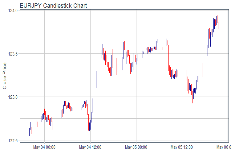
Fig.1. Chart of quotes
Draw the FATL, SATL, RFTL, RSTL and ZZ:chart
evalq(pr %>% tail(., 200) %>%
        ggplot(aes(x = Data, y = Close)) +
        geom_candlestick(aes(open = Open, high = High, low = Low, close = Close)) +
        geom_line(aes(Data, fatl), color = "steelblue", size = 1) +
        geom_line(aes(Data, rftl), color = "red", size = 1) +
        geom_line(aes(Data, satl), color = "gold", size = 1) +
        geom_line(aes(Data, rstl), color = "green", size = 1) +
        geom_line(aes(Data, zigz), color = "black", size = 1) +
        labs(title = "EURJPY Candlestick Chart",
             subtitle = "Combining Chart Geoms",
             y = "Close Price", x = "") +
        theme_tq(), env)
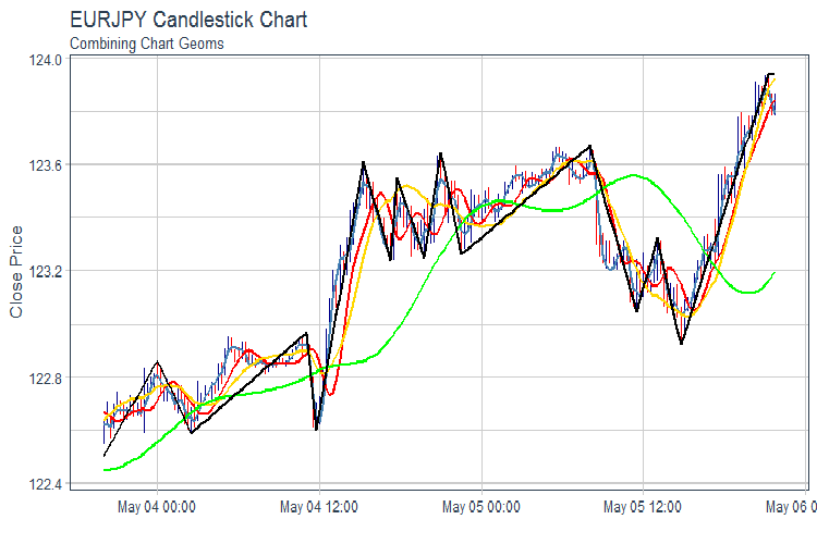
Fig.2. FATL, SATL, RFTL, RSTL and ZZ
Split oscillators into three groups for more convenient representation.
require(dygraphs)
evalq(dataSet %>% tail(., 200) %>% tk_tbl %>%
        select(Data, ftlm, stlm, rbci, pcci) %>%
        tk_xts() %>%
        dygraph(., main = "Oscilator base") %>%
        dyOptions(.,
                  fillGraph = TRUE,
                  fillAlpha = 0.2,
                  drawGapEdgePoints = TRUE,
                  colors = c("green", "violet", "red", "blue"),
                  digitsAfterDecimal = Dig) %>%
        dyLegend(show = "always",
                 hideOnMouseOut = TRUE),
      env)
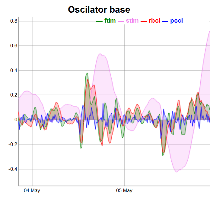
Fig.3. Base oscillators
evalq(dataSet %>% tail(., 200) %>% tk_tbl %>%
        select(Data, v.fatl, v.satl, v.rftl, v.rstl) %>%
        tk_xts() %>%
        dygraph(., main = "Oscilator 2") %>%
        dyOptions(.,
                  fillGraph = TRUE,
                  fillAlpha = 0.2,
                  drawGapEdgePoints = TRUE,
                  colors = c("green", "violet", "red", "darkblue"),
                  digitsAfterDecimal = Dig) %>%
        dyLegend(show = "always",
                 hideOnMouseOut = TRUE),
      env)
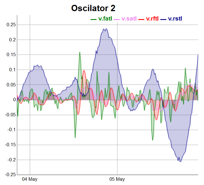
Fig.4. Oscillators of the second group
Oscillators of the third group will be drawn on the last 100 bars:
evalq(dataSet %>% tail(., 100) %>% tk_tbl %>%
        select(Data, v.ftlm, v.stlm, v.rbci, v.pcci) %>%
        tk_xts() %>%
        dygraph(., main = "Oscilator 3") %>%
        dyOptions(.,
                  fillGraph = TRUE,
                  fillAlpha = 0.2,
                  drawGapEdgePoints = TRUE,
                  colors = c("green", "violet", "red", "darkblue"),
                  digitsAfterDecimal = Dig) %>%
        dyLegend(show = "always",
                 hideOnMouseOut = TRUE),
      env)
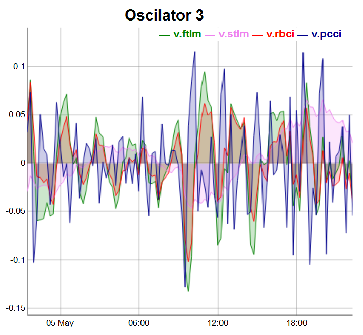
Fig.5. Oscillators of the third group
2.Exploratory data analysis, EDA
“There are no trivial statistical questions, there are dubious statistical procedures.” — Sir David Cox
“An approximate answer to the right problem is worth a good deal more than an exact answer to an approximate problem.” — John Tukey
We are using EDA to develop the understanding of the data in use. The simplest way to do this is to use questions as the research tool. When we ask a question, we are focused on a certain part of the data. This will help to decide what charts, models and transformations to use.
EDA is essentially a creative process. Similar to most creative processes, the key to asking a good question is creating even more questions. It is difficult to ask fundamental questions at the beginning of analysis as we do not know what conclusions the data set contains. On the other hand, every new question we ask, highlights a new aspect of data and increases our chances to make a discovery. We can quickly move to the most interesting part of the data set and clarify the situation by asking sequential questions.
There are no rules for what questions we should ask to study the data. Having said that, there are two types of questions that will be useful:
-
What type of change are my variables undergoing?
- What type of covariation is occurring between variables?
Let us define the principle concept.
Variations are a tendency for values of a variable to change at different measurements. There are plenty of examples of variations in everyday life. If you measure any continuous variable seven times, you will get seven different values. This is true even for constants, for example the speed of light. Each measurement will contain small errors which will be different every time. Variables of the same type can change too. For instance, the eye color of different people or electron energy level at different time. Each variable has its own character of variations which can reveal interesting information. The best way to understand this information is to visualize the distribution of the variable values. This is a case when one diagram is better than a thousand words.
2.1.Total statistics
The total statistics of a timeseries is convenient to track using the table.Stats()::PerformenceAnalitics function.
> table.Stats(env$dataSet %>% tk_xts())
Using column `Data` for date_var.
                     ftlm      stlm      rbci      pcci
Observations    7955.0000 7908.0000 7934.0000 7960.0000
NAs               42.0000   89.0000   63.0000   37.0000
Minimum           -0.7597   -1.0213   -0.9523   -0.5517
Quartile 1        -0.0556   -0.1602   -0.0636   -0.0245
Median            -0.0001    0.0062   -0.0016   -0.0001
Arithmetic Mean    0.0007    0.0025    0.0007    0.0001
Geometric Mean    -0.0062       NaN   -0.0084   -0.0011
Quartile 3         0.0562    0.1539    0.0675    0.0241
Maximum            2.7505    3.0407    2.3872    1.8859
SE Mean            0.0014    0.0033    0.0015    0.0006
LCL Mean (0.95)   -0.0020   -0.0040   -0.0022   -0.0010
UCL Mean (0.95)    0.0034    0.0090    0.0035    0.0012
Variance           0.0152    0.0858    0.0172    0.0026
Stdev              0.1231    0.2929    0.1311    0.0506
Skewness           4.2129    1.7842    2.3037    6.4718
Kurtosis          84.6116   16.7471   45.0133  247.4208
                   v.fatl    v.satl    v.rftl    v.rstl
Observations    7959.0000 7933.0000 7954.0000 7907.0000
NAs               38.0000   64.0000   43.0000   90.0000
Minimum           -0.3967   -0.0871   -0.1882   -0.4719
Quartile 1        -0.0225   -0.0111   -0.0142   -0.0759
Median            -0.0006    0.0003    0.0000    0.0024
Arithmetic Mean    0.0002    0.0002    0.0002    0.0011
Geometric Mean    -0.0009    0.0000   -0.0003   -0.0078
Quartile 3         0.0220    0.0110    0.0138    0.0751
Maximum            1.4832    0.3579    0.6513    1.3093
SE Mean            0.0005    0.0002    0.0003    0.0015
LCL Mean (0.95)   -0.0009   -0.0003   -0.0005   -0.0020
UCL Mean (0.95)    0.0012    0.0007    0.0009    0.0041
Variance           0.0023    0.0005    0.0009    0.0188
Stdev              0.0483    0.0219    0.0308    0.1372
Skewness           5.2643    2.6705    3.9472    1.5682
Kurtosis         145.8441   36.9378   74.4182   13.5724
                   v.ftlm    v.stlm    v.rbci    v.pcci
Observations    7954.0000 7907.0000 7933.0000 7959.0000
NAs               43.0000   90.0000   64.0000   38.0000
Minimum           -0.9500   -0.2055   -0.6361   -1.4732
Quartile 1        -0.0280   -0.0136   -0.0209   -0.0277
Median            -0.0002   -0.0001   -0.0004   -0.0002
Arithmetic Mean    0.0000    0.0001    0.0000    0.0000
Geometric Mean    -0.0018   -0.0003   -0.0009       NaN
Quartile 3         0.0273    0.0143    0.0207    0.0278
Maximum            1.4536    0.3852    1.1254    1.9978
SE Mean            0.0006    0.0003    0.0005    0.0006
LCL Mean (0.95)   -0.0012   -0.0005   -0.0009   -0.0013
UCL Mean (0.95)    0.0013    0.0007    0.0009    0.0013
Variance           0.0032    0.0007    0.0018    0.0034
Stdev              0.0561    0.0264    0.0427    0.0579
Skewness           1.2051    0.8513    2.0643    3.0207
Kurtosis          86.2425   23.0651   86.3768  233.1964
Here is what this table tells us:
- All predictors have a relatively small number of undefined variables NA.
- All predictors have a pronounced right skewness.
- All predictors have a high kurtosis.
2.2.Visualizing total statistics
“The greatest value of a picture is when it forces us to notice what we never expected to see”. — John Tukey
Let us see the variation and covariation between the variables in the dataSet. As the number of variables (14) would not allow us to represent them on one chart, they will have to be split into three groups.
require(GGally)
evalq(ggpairs(dataSet, columns = 2:6,
              mapping = aes(color = Class),
              title = "DigFilter1"),
      env)
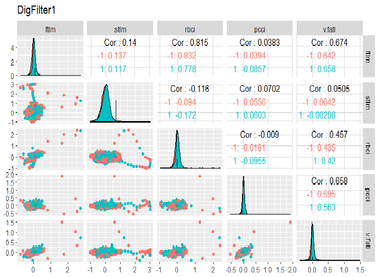
Fig. 6. First group of predictors
evalq(ggpairs(dataSet, columns = 7:10,
              mapping = aes(color = Class),
              title = "DigFilter2"),
      env)
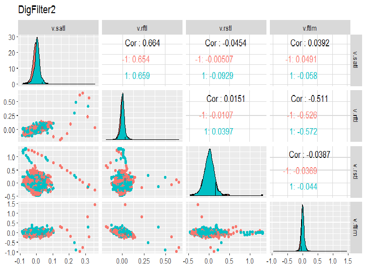
Fig. 7. Second group of predictors
evalq(ggpairs(dataSet, columns = 11:14,
              mapping = aes(color = Class),
              title = "DigFilter3"),
      env)
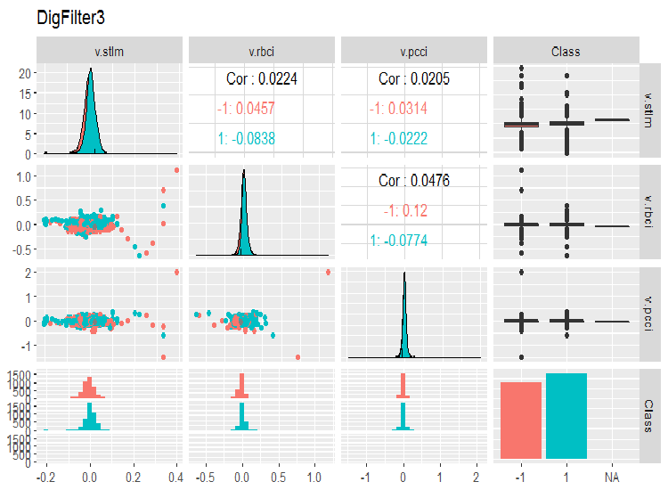
Fig. 8. Third group of predictors
This is what we should see on the charts:
- all predictors have the shape of distributions close to normal, though there is a well pronounced right skewness;
- all predictors have a very narrow interquartile range (IQR);
- all predictors have prominent outliers;
- the number of examples at two levels of the goal variable "Class” have a small difference.
3.Preparing data
Normally, preparing data has seven stages:
- “imputation” — removing or imputing missed/undefined data;
- “variance” — removing variables with zero or near-zero dispersion;
- “split” — dividing the data set into the train/valid/test subsets;
- “scaling” — scaling the range of variables;
- “outliers” — removing or imputing outliers;
- “sampling” — correcting the class imbalance;
- “denoise” — removing or redefining noise;
- “selection” — selecting irrelevant predictors.
3.1. Data cleaning
The first stage of preparing raw data is removing or imputing undefined values and gaps in the data. Although many models allow using undefined data (NA) and gaps in data sets, they are best deleted before starting the main actions. This operation is carried out for the full data set regardless of the model.
The total statistics of our raw data indicated that the data set contains NA. These are artificial A, which appeared when calculating digital filters. There are not many of them so they can be deleted. We have already obtained the dataSet ready for further processing. Let us clean it.
In a general case, cleaning means the following operations:
- removing predictors with a zero or near zero dispersion (method = c(“zv”, “nzv”));
- removing highly correlated variables. It is up to the user to set the threshold for coefficient of correlation (method = “corr”). Its default value is 0.9. This stage is not always necessary. It depends on the following methods of transformation;
- removing predictors that have only one unique value in any class (method = “conditionalX”).
All these operations are implemented in the preProcess()::caret function by means of the methods considered above. These operations are carried out for the complete data set before the division into the training and test sets.
require(caret)
evalq({preProClean <- preProcess(x = dataSet,method = c("zv", "nzv", "conditionalX", "corr"))
      dataSetClean <- predict(preProClean, dataSet %>% na.omit)},
env)
Let us see if there are any deleted predictors and what we have after cleaning:
> env$preProClean$method$remove
#[1] "v.rbci"
> dim(env$dataSetClean)
[1] 7906   13
> colnames(env$dataSetClean)
 [1] "Data"   "ftlm"   "stlm"   "rbci"   "pcci"
 [6] "v.fatl" "v.satl" "v.rftl" "v.rstl" "v.ftlm"
[11] "v.stlm" "v.pcci" "Class"
3.2. Identifying and processing outliers
Problems with the quality of data such as skewness and outliers are often interconnected and interdependent. This does not only make a preliminary processing of data time consuming but also makes finding correlations and tendencies in the data set difficult.
What are outliers?
Let us agree that an outlier is an observation that is too distant from other observations. A detailed classification of outliers, methods of their identification and processing is described in [2].
Types of outliers
Outliers cause significant distortions in the distribution of variables and training a model using such data. There are many methods of identifying and processing outliers. The choice of method mainly depends on whether we identify the outlier locally or globally. Local outliers are outliers of one variable. Global outliers are outliers in a multidimensional space defined either by a matrix or a dataframe.
What causes outliers?
Outliers can be divided by origin:
Artificial
- errors of the data entry. Here belong the errors occurred during the collection, recording and processing of data;
- experimental errors;
- sampling errors.
Natural errors caused by the nature of the variable.
What impact do outliers have?
Outliers can ruin results of data analysis and statistical modeling. This increases error dispersion and decreases statistical power of tests. If outliers are not distributed randomly, they can reduce normality. Outliers can also influence main assumption of regression and dispersion analyses along with other statistical assumptions of the model.
How can we identify local outliers?
Usually outliers can be revealed by visualizing data. One of the most simple and widely used methods is boxplot. Let us take the ftlm predictor as an example:
evalq(ggplot(dataSetClean, aes(x = factor(0),
                               y = ftlm,
                               color = 'red')) +
        geom_boxplot() + xlab("") +
        scale_x_discrete(breaks = NULL) +
        coord_flip(),
      env)
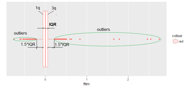
Fig.9. Boxplot ftlm
Some comments to the diagram:
IQR is the interquartile range or the distance between the first and the third quartile.
This way, we can define outliers in several ways:
- Any value smaller than -1.5*IQR and greater than +1.5*IQR is an outlier. Sometimes, the coefficient is set to 2 or 3. All values between 1.5*IQR and 3*IQR are called mean outliers and the values above 3*IQR are called extreme outliers.
- Any value that appears to be outside of the 5th and 95th percentile can be considered to be an outlier,
- Points plotted three or more MSD away are also outliers.
Going forward, we are going to use the first definition of outliers - through IQR.
How can outliers be processed?
Most methods of processing outliers are similar to the methods of processing of NA - removing observations, transforming observations, segmenting, imputing and others.
- Removing outliers. We remove the value of outliers if they appear as a result of the data entry error or if the number of outliers is very small. We can also trim the ends of the distribution to remove outliers. For example, we can discard 1% from the top and bottom.
- Transformation and binning:
- transformation of variables can exclude outliers (this will be looked into in the next part of the article);
- natural logarithm diminishes the changes cased by the extreme values (this will also be discussed in detail in the next part of the article);
- discretization is also a way of transforming a variable (see the next part);
- we can also use weight assignment to observations (we will not discuss this in this article).
Imputation. Same methods that we use for imputing undefined values can be used for imputing outliers. For that the mean, median and mode can be used. Before imputing values, it is necessary to establish if the outlier is natural or artificial. If the outlier is artificial, it can be imputed.
If the sample contains a significant number of outliers, they should be analyzed separately in a statistical model. We are going to discuss general methods used to tackle outliers. They are removal and imputation.
Removing outliers
The outliers must be deleted if they are caused by the data entry, processing data or the number of outliers is very small (only when identifying statistical variable metrics).
Data of one variable (ftlm, for instance) can be extracted without outliers as follows:
evalq({dataSetClean$ftlm -> x
  out.ftlm <- x[!x %in% boxplot.stats(x)$out]},
  env)
Or:
evalq({dataSetClean$ftlm -> x
  out.ftlm1 <- x[x > quantile(x, .25) - 1.5*IQR(x) &
          x < quantile(x, .75) + 1.5*IQR(x)]},
  env)
Are they identical?
> evalq(all.equal(out.ftlm, out.ftlm1), env)
[1] TRUE
How many outliers are there in the data set?
> nrow(env$dataSetClean) - length(env$out.ftlm)
[1] 402
This is what ftlm looks without outliers:
boxplot(env$out.ftlm, main = "ftlm  without outliers",
        boxwex = 0.5)
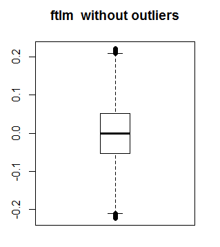
Fig. 10. ftlm without outliers
The method described above is not suitable for matrices and dataframes as every variable in a dataframe can have a different number of outliers. A method of substituting local outliers for NA followed by standard methods of processing NA is suitable for such samples. The function that will substitute local outliers for NA is shown below:
#-------remove_outliers-------------------------------
remove_outliers <- function(x, na.rm = TRUE, ...) {
  qnt <- quantile(x, probs = c(.25, .75),
                  na.rm = na.rm, ...)
  H <- 1.5 * IQR(x, na.rm = na.rm)
  y <- x
  y[x < (qnt[1] - H)] <- NA
  y[x > (qnt[2] + H)] <- NA
  y
}
Let us change dataSetClean in all variables, except c(Data, Class), and outliers for NA. Having done that, let us see how the distribution of the new set x.out: changes.
evalq({
  dataSetClean %>% select(-c(Data,Class)) %>% as.data.frame() -> x
  foreach(i = 1:ncol(x), .combine = "cbind") %do% {
    remove_outliers(x[ ,i])
  } -> x.out
  colnames(x.out) <- colnames(x)
  },
env)
par(mfrow = c(1, 1))
chart.Boxplot(env$x,
              main = "x.out with outliers",
              xlab = "")
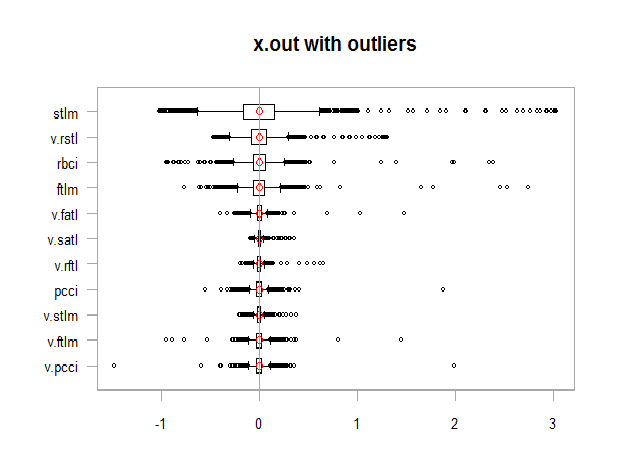
Fig. 11. Data with outliers
chart.Boxplot(env$x.out,
              main = "x.out without outliers",
              xlab = "")
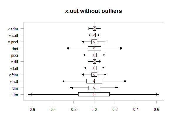
Fig.12. Data without outliers
Imputing NA that appeared instead of outliers
Imputation is a substitution of missing, incorrect or invalid values with other values. The input data for training the model must contain only valid values. You can either:
- substitute NA for the mean, median, mod (the statistical characteristics of the set will not change)
- substitute the outliers greater than 1.5*IQR for 0.95 percentile and the outliers smaller than - 1.5*IQR for 0.05 percentile.
Let us write a function to perform the last version of the action. After the transformation has been done, let us take a look at the distribution:
#-------capping_outliers-------------------------------
capping_outliers <- function(x, na.rm = TRUE, ...) {
  qnt <- quantile(x, probs = c(.25, .75),
                  na.rm = na.rm, ...)
  caps <- quantile(x, probs = c(.05, .95),
                   na.rm = na.rm, ...)
  H <- 1.5 * IQR(x, na.rm = na.rm)
  y <- x
  y[x < (qnt[1] - H)] <- caps[1]
  y[x > (qnt[2] + H)] <- caps[2]
  y
}

evalq({dataSetClean %>% select(-c(Data,Class)) %>%
    as.data.frame() -> x
    foreach(i = 1:ncol(x), .combine = "cbind") %do% {
      capping_outliers(x[ ,i])
    } -> x.cap
    colnames(x.cap) <- colnames(x)
   },
env)
chart.Boxplot(env$x.cap,
              main = "x.cap with capping outliers",
              xlab = "")
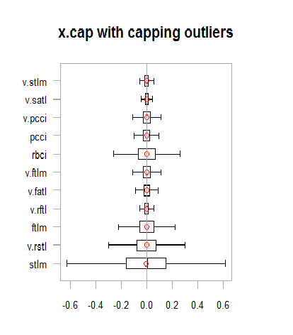
Fig.13. Data set with imputed outliers
Let us consider the variation and covariation in dataSetCap . This is the same as dataSet but cleaned and containing imputed local outliers. The number of variables (13) makes it impossible to put them on the same chart, so they will have to be split into two groups.
evalq(x.cap %>% tbl_df() %>%
        cbind(Data = dataSetClean$Data, .,
              Class = dataSetClean$Class) ->
        dataSetCap,
      env)
require(GGally)
evalq(ggpairs(dataSetCap, columns = 2:7,

              mapping = aes(color = Class),
              title = "PredCap1"),
      env)
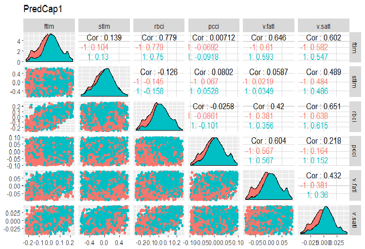
Fig.14. Variation and covariation of the first part of the data set with imputed outliers.
And the second part of the set:
evalq(ggpairs(dataSetCap, columns = 8:13,
              mapping = aes(color = Class),
              title = "PredCap2"),
      env)
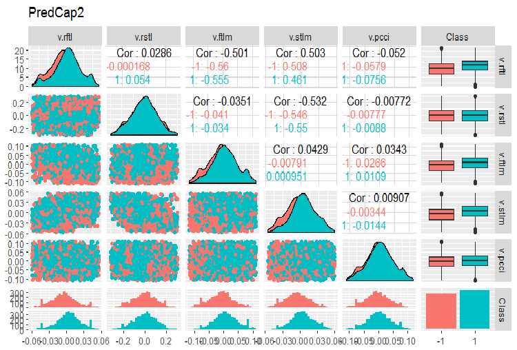
Fig.15. Variation and covariation of the second part of the data set with imputed outliers
How can global outliers be identified?
Two-dimensional or multi-dimensional outliers are usually identified using the impact or proximity index. Various distances are used for identifying global outliers. Packages like DMwR, mvoutliers, Rlof can be used for that. Global outliers are evaluated with LOF (local outlier factor). Calculate and compare LOF for a set with outliers x and a set with imputed outliers x.cap.
##------DMwR2-------------------
require(DMwR2)
evalq(lof.x <- lofactor(x,10), env)
evalq(lof.x.cap <- lofactor(x.cap,10), env)
par(mfrow = c(1, 3))
boxplot(env$lof.x, main = "lof.x",
        boxwex = 0.5)
boxplot(env$lof.x.cap, main = "lof.x.cap",
        boxwex = 0.5)
hist(env$lof.x.cap, breaks = 20)
par(mfrow = c(1, 1))
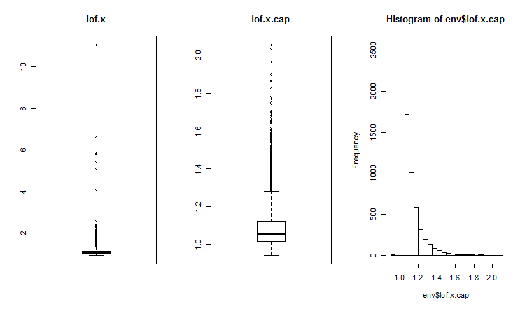
Fig.16. Global outlier factor for a data set with outliers and a data set with imputed outliers
The lof() function is implemented in the Rlof package. It finds the local outlier factor[3] of matrix data using k nearest neighbors. Local outlier factor (LOF) is a probability of belonging to outliers which is calculated for every observation. Based on this probability, the user decides if the observation is an outlier.
LOF takes into account local density to identify if the observation is an outlier. This is a more efficient implementation of LOF using another structure of data and functions of calculation of distance to compare with the lofactor() function available in the “dprep” package. This will be supporting several values of k which will be calculated simultaneously, and various measures of distance in addition to the standard Euclidean one. The calculations are done simultaneously on several cores of the processor. Let us calculate the lofactor for the same two sets (x and x.cap) for 5, 6, 7, 8, 9 and 10 neighbours using the “minkowski” method of calculating distance. Let us draw histograms of these lofactors.
require(Rlof)
evalq(Rlof.x <- lof(x, c(5:10), cores = 2,
                       method = 'minkowski'),
        env)
  evalq(Rlof.x.cap <- lof(x.cap, c(5:10),
                          cores = 2,
                          method = 'minkowski'),
        env)
par(mfrow = c(2, 3))
hist(env$Rlof.x.cap[ ,6], breaks = 20)
hist(env$Rlof.x.cap[ ,5], breaks = 20)
hist(env$Rlof.x.cap[ ,4], breaks = 20)
hist(env$Rlof.x.cap[ ,3], breaks = 20)
hist(env$Rlof.x.cap[ ,2], breaks = 20)
hist(env$Rlof.x.cap[ ,1], breaks = 20)
par(mfrow = c(1, 1))
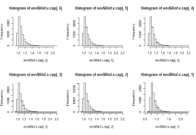
Fig.17. Global outlier factor for k neighbours
Nearly all observations are within the range lofactor =1.6. Outside of this range:
> sum(env$Rlof.x.cap[ ,6] >= 1.6)
[1] 32
This is an insignificant number of moderate outliers for a set of this size.
Note. To identify the range limits, exceeding which the observation will be treated as an outlier, one should use a training data set. The value of the variables of the test/validation data set are processed using the parameters obtained by means of the training set. What parameters are these? These are the limits upper = 1.5*IQR, lower = -1.5*IQR and cap =c(0.05, 0.95) percentile. We used them in our earlier calculations. If other methods of calculating the limits of the range and imputation of outliers were used, they must be defined for the training data set, saved and stored for processing the validation and test data sets.
Let us write the function that will perform preliminary calculations:
#-----prep.outlier--------------
prep.outlier <- function(x, na.rm = TRUE, ...) {
  qnt <- quantile(x, probs = c(.25, .75),
                  na.rm = na.rm, ...)
  H <- 1.5 * IQR(x, na.rm = na.rm)
  caps <- quantile(x, probs = c(.05, .95),
                   na.rm = na.rm, ...)
  list(lower = qnt[1] - H, upper = qnt[2] + H,
       med = median(x),
       cap1 = caps[1], cap2 = caps[2])
}
Calculate parameters required for identifying and imputing outliers. Let the preliminary length of the training set be first 4000 bars and the following 2000 bars will be used as the test data set.
evalq(
  {train <- x[1:4000, ]
  foreach(i = 1:ncol(train), .combine = "cbind") %do% {
    prep.outlier(train[ ,i]) %>% unlist()
  } -> pre.outl
  colnames(pre.outl) <- colnames(x)
  #pre.outl %<>% t()
  },
  env)
Let us look at the result:
> env$pre.outl
                   ftlm        stlm         rbci          pcci
lower.25% -0.2224942912 -0.59629203 -0.253231002 -9.902232e-02
upper.75%  0.2214486206  0.59242529  0.253529797  9.826936e-02
med       -0.0001534451  0.00282525 -0.001184966  8.417127e-05
cap1.5%   -0.1700418145 -0.40370452 -0.181326658 -6.892085e-02
cap2.95%   0.1676526431  0.39842675  0.183671973  6.853935e-02
                 v.fatl        v.satl        v.rftl        v.rstl
lower.25% -0.0900973332 -4.259328e-02 -0.0558921804 -0.2858430788
upper.75%  0.0888110249  4.178418e-02  0.0555115004  0.2889057397
med       -0.0008581219 -2.130064e-05 -0.0001707447 -0.0001721546
cap1.5%   -0.0658731640 -2.929586e-02 -0.0427927888 -0.1951978435
cap2.95%   0.0662353821  3.089833e-02  0.0411091859  0.1820803387
                 v.ftlm        v.stlm        v.pcci
lower.25% -0.1115823754 -5.366875e-02 -0.1115905239
upper.75%  0.1108670403  5.367466e-02  0.1119495436
med       -0.0003560178 -6.370034e-05 -0.0003173464
cap1.5%   -0.0765431363 -3.686945e-02 -0.0765950814
cap2.95%   0.0789209957  3.614423e-02  0.0770439553
As we can see, first and third quartiles and median along with 5th and 95th percentile are defined for every variable in the set. This is everything that is required for identifying and processing outliers.
We need a function to process outliers of any data set using previously set parameters. Possible ways of processing: substituting outliers for NA, substituting outliers for the median and substituting outliers for 5th/95th percentile.
#---------treatOutlier---------------------------------
  treatOutlier <- function(x, impute = TRUE, fill = FALSE,
                         lower, upper, med, cap1, cap2){
  if (impute) {
    x[x < lower] <- cap1
    x[x > upper] <- cap2
    return(x)
  }
  if (!fill) {
    x[x < lower | x > upper] <- NA
    return(x)
  } else {
    x[x < lower | x > upper] <- med
    return(x)
  }
}
As we defined required parameters for the training set, let us process outliers of the training set having substituted them for the 5th/95th percentile. Then process outliers of the test data set. Compare distributions in the obtained sets having plotted three charts.
#------------
evalq(
  {
  foreach(i = 1:ncol(train), .combine = 'cbind') %do% {
    stopifnot(exists("pre.outl", envir = env))
    lower = pre.outl['lower.25%', i]
    upper = pre.outl['upper.75%', i]
    med = pre.outl['med', i]
    cap1 = pre.outl['cap1.5%', i]
    cap2 = pre.outl['cap2.95%', i]
    treatOutlier(x = train[ ,i], impute = T, fill = T, lower = lower,
                 upper = upper, med = med, cap1 = cap1, cap2 = cap2)
  } -> train.out
  colnames(train.out) <- colnames(train)
  },
  env
)
#-------------
evalq(
  {test <- x[4001:6000, ]
  foreach(i = 1:ncol(test), .combine = 'cbind') %do% {
    stopifnot(exists("pre.outl", envir = env))
    lower = pre.outl['lower.25%', i]
    upper = pre.outl['upper.75%', i]
    med = pre.outl['med', i]
    cap1 = pre.outl['cap1.5%', i]
    cap2 = pre.outl['cap2.95%', i]
    treatOutlier(x = test[ ,i], impute = T, fill = T, lower = lower,
                 upper = upper, med = med, cap1 = cap1, cap2 = cap2)
  } -> test.out
  colnames(test.out) <- colnames(test)
  },
  env
)
#---------------
evalq(boxplot(train, main = "train  with outliers"), env)
evalq(boxplot(train.out, main = "train.out  without outliers"), env)
evalq(boxplot(test.out, main = "test.out  without outliers"), env)
#------------------------
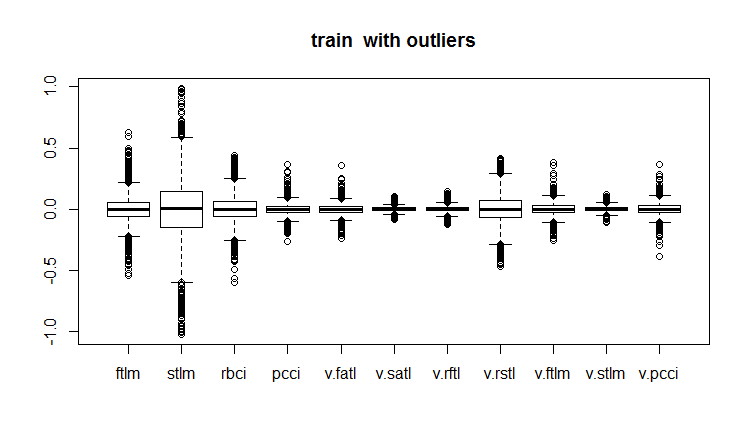
Fig.18. Training data set with outliers
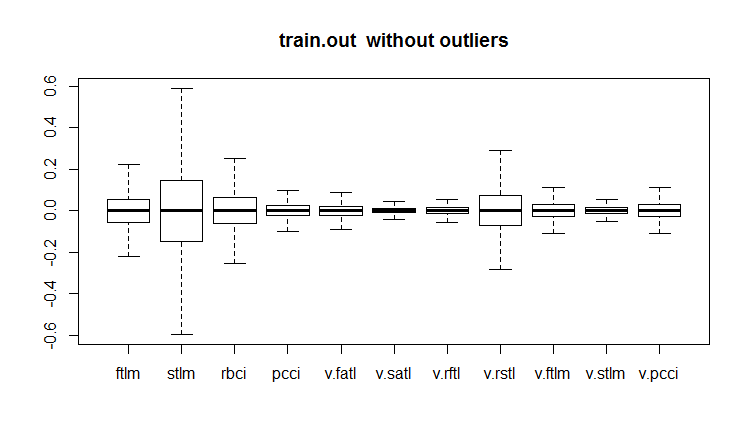
Fig.19. Training data set with imputed outliers
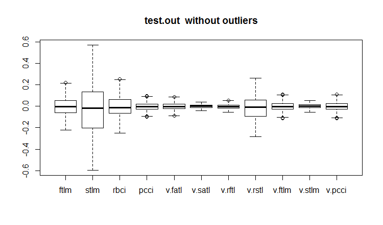
Fig.20. Test data set with imputed outliers
Not all models are sensitive to outliers. For instance, such models as determining trees (DT) and random forests(RF) are insensitive to them.
When defining and processing outliers, some other packages may be useful. They are: “univOutl”, “mvoutlier”, “outlier”, funModeling::prep.outlier().
3.3. Eliminating skewness
Skewness is the indication of the form of the distribution. Calculating the skewness coefficient of a variable is a general way of assessing this. Usually, negative skewness shows that the mean is smaller than the median and the distribution has left skewness. Positive skewness indicates that the mean is greater than the median and the distribution has right skewness.
If the predictor skewness is 0, then the data are absolutely symmetrical.
If the predictor skewness is less than -1 or greater than +1, then the data are significantly distorted.
If the predictor skewness is between -1 and -1/2 or +1 and +1/2, then the data are moderately distorted.
If the predictor skewness is equal to -1/2 and +1/2, the data are close to symmetrical.
The right skewness can be corrected by taking logarithms and the left skewness by using the exponential function.
We have established that skewness, outliers and other transformations are connected. Let us see how the index of skewness changed after removing and imputing outliers.
evalq({
  sk <- skewness(x)
  sk.out <- skewness(x.out)
  sk.cap <- skewness(x.cap)
  },
  env)
> env$sk
             ftlm     stlm     rbci     pcci   v.fatl
Skewness 4.219857 1.785286 2.304655 6.491546 5.274871
           v.satl   v.rftl   v.rstl   v.ftlm    v.stlm
Skewness 2.677162 3.954098 1.568675 1.207227 0.8516043
           v.pcci
Skewness 3.031012
> env$sk.out
                ftlm        stlm        rbci       pcci
Skewness -0.04272076 -0.07893945 -0.02460354 0.01485785
             v.fatl      v.satl      v.rftl      v.rstl
Skewness 0.00780424 -0.02640635 -0.04663711 -0.04290957
                v.ftlm     v.stlm       v.pcci
Skewness -0.0009597876 0.01997082 0.0007462494
> env$sk.cap
                ftlm        stlm        rbci       pcci
Skewness -0.03329392 -0.07911245 -0.02847851 0.01915228
             v.fatl      v.satl      v.rftl      v.rstl
Skewness 0.01412182 -0.02617518 -0.03412228 -0.04596505
              v.ftlm      v.stlm      v.pcci
Skewness 0.008181183 0.009661169 0.002252508
As you can see, both the set with removed outliers x.out and the one with imputed outliers x.cap are absolutely symmetrical and do not require any correction.
Let us assess kurtosis too. Kurtosis or coefficient of peakedness is a measure of peakedness of a random variable distribution. The kurtosis of a normal distribution is 0. Kurtosis is positive if the peak of the distribution around mathematical expectation is sharp and negative is the peak is smooth.
require(PerformanceAnalytics)
evalq({
  k <- kurtosis(x)
  k.out <- kurtosis(x.out)
  k.cap <- kurtosis(x.cap)
},
env)
> env$k
                    ftlm     stlm     rbci     pcci
Excess Kurtosis 84.61177 16.77141 45.01858 247.9795
                  v.fatl   v.satl  v.rftl   v.rstl
Excess Kurtosis 145.9547 36.99944 74.4307 13.57613
                  v.ftlm   v.stlm   v.pcci
Excess Kurtosis 86.36448 23.06635 233.5408
> env$k.out
                        ftlm       stlm       rbci
Excess Kurtosis -0.003083449 -0.1668102 -0.1197043
                       pcci      v.fatl      v.satl
Excess Kurtosis -0.05113439 -0.02738558 -0.04341552
                     v.rftl     v.rstl     v.ftlm
Excess Kurtosis -0.01219999 -0.1316499 -0.0287925
                    v.stlm      v.pcci
Excess Kurtosis -0.1530424 -0.09950709
> env$k.cap
                      ftlm       stlm       rbci
Excess Kurtosis -0.2314336 -0.3075185 -0.2982044
                      pcci     v.fatl     v.satl
Excess Kurtosis -0.2452504 -0.2389486 -0.2331203
                    v.rftl     v.rstl     v.ftlm
Excess Kurtosis -0.2438431 -0.2673441 -0.2180059
                    v.stlm     v.pcci
Excess Kurtosis -0.2763058 -0.2698028
Peaks of the distribution in the initial data set x are very sharp (kurtosis is much greater than 0) In the set with removed outliers x.out, peaks are very close to the normal peakedness. The set with imputed outliers has more smooth peaks. Both data sets do not require any corrections.
Application
1. The DARCH12_1.zip archive contains the scripts for the first part of the article (dataRaw.R, PrepareData.R, FUNCTION.R) and a diagram representing the Rstudio session with the initial data Cotir.RData. Load the data into Rstudio and you will be able to see all the scripts and work with them. You can also download it from Git /Part_I.
2. The ACTF.zip archive contains the article by V. Kravchuk "New Adaptive Method of Following the Tendency and Market Cycles"
3. The R_intro.zip archive contains reference materials on R.
Links
[1] A Systematic Approach on Data Pre-processing In Data Mining. COMPUSOFT, An international journal of advanced computer technology, 2 (11), November-2013 (Volume-II, Issue-XI)
[2] Outlier Detection Techniques.Hans-Peter Kriegel, Peer Kröger, Arthur Zimek. Ludwig-Maximilians-Universität München.Munich, Germany
[3] Breuning, M., Kriegel, H., Ng, R.T, and Sander. J. (2000). LOF: Identifying density-based local outliers. In Proceedings of the ACM SIGMOD International Conference on Management of Data.
Translated from Russian by MetaQuotes Ltd.
Original article: https://www.mql5.com/ru/articles/3486
Warning: All rights to these materials are reserved by MetaQuotes Ltd. Copying or reprinting of these materials in whole or in part is prohibited.
This article was written by a user of the site and reflects their personal views. MetaQuotes Ltd is not responsible for the accuracy of the information presented, nor for any consequences resulting from the use of the solutions, strategies or recommendations described.
 Cross-Platform Expert Advisor: Stops
- Free trading apps
- Over 8,000 signals for copying
- Economic news for exploring financial markets
You agree to website policy and terms of use
Hello, as following your article (1st time touching R), right in the 2nd brick of code I was faced with the folllwing error :
Error in evalq({ : object 'env' not found
does env here means something named in the pc software ? Or it is really a object that was created automatically?
Awesome article, gonna find a way to surpass it, would be awesome if you could help :)
(Using RStudio and installed MRO 3.5.3 (because 3.4.0 was outdated))
Hello, following your article (touching R for the first time), right in the second block of code, I ran into the following error:
Error in evalq ({: object 'env' not found
here env means something named in pc software? Or is it really an auto-generated object?
Great article, I will find a way to beat it, it would be great if you could help :)
(Using RStudio and installing MRO 3.5.3 (since 3.4.0 is deprecated))
The env object was created to separate data from various tools. Just at the beginning of the script write
Good luck.
Dear MR. Vladimir Perervenko, thank you a lot for your fast answer, after taking a R course I hope to make at least enough to deserve the study of your awesome work, thank you a lot for sharing Mr. Vladimir.
Best of best Regards
Ferox
Hello again Mr. Perervenko, hope you are feeling great. I have a new question, when you first wrote about ZigZag :
on the 9th line, what's the meaning of the Dig object?
Couldn't find it on the project or in the required packages ...
Best Regards MR. Perervenko
Ferox
I'm sorry my stupid question Mr. Vladimir Perervenko.
Already solved it, there's no excuses
Best regards