
Deep Neural Networks (Part IV). Creating, training and testing a model of neural network
Contents
- Introduction
- 1. Brief description of the package capabilities
- 1.1. Initialization functions of neurons
- 1.2. Activation functions of neurons
- 1.3. Training methods
- 1.4. Methods of regulation and stabilization
- 1.5. Methods and parameters of training an RBM
- 1.6. Methods and parameters of training a DNN
- 2. Testing the quality of work of a DNN depending on the used parameters
- 2.1. Experiments
- 2.1.1. Input data (preparation)
- 2.1.2. Basic model of comparison
- 2.1.3. Structure of a DNN
- 2.1.4. Variants of training
- 2.2. Result analysis
- Conclusion
- Application
Introduction
Main directions of study and application
Currently, there are two main streams in study and application of deep neural networks. They differ in the approach to the initialization of the neuron weights in hidden layers.
Approach 1. Neural networks are very sensitive to the method of the initialization of neurons in hidden layers, especially if the number of hidden layers increases (greater than 3). Professor G.Hynton was the first to try and solve this problem. The idea behind his approach was to initiate the weights of neurons in hidden layers with the weights obtained during unsupervised training of autoassociative neural networks made up of RBM (restricted Boltzmann machine) or AE (autoencoder). These stacked RBM (SRBM) and stacked AE (SAE) are trained with a large array of unlabeled data. The aim of such training is to highlight hidden structures (representations, images) and relationships in the data. Initialization of neurons with MLP weights, obtained during the pretraining puts the MLP to the space of solutions very close to the optimal one. This allows to decrease the number of labeled data and the epochs during the following fine tuning (training) of MLP. These are extremely important advantages for many spheres of practical application, especially when processing a lot of data.
Approach 2: Another group of scientists headed by Yoshua Benjio created specific methods of initialization of hidden neurons, specific functions of activation, methods of stabilization and training. The success of this direction is connected with an extensive development of deep convolutional neural networks and recurrent neural networks (DCNN, RNN). Such neural networks showed high efficiency in image recognition, analysis and classification of texts along with translation of spoken speech from one language into another. Ideas and methods, developed for these neural networks also started to be used for MLP.
Currently, both approaches are actively used. It should be noted that with nearly same results, neural networks with pretraining require less computational resources and fewer samples for training. This is an important advantage. I personally favor deep neural networks with pretraining. I believe that the future belongs to the unsupervised learning.
Packages in R that allow to develop and use DNN
R has a number of packages for creating and using DNN with a different level of complexity and set of capabilities.
Packages allowing to create, train and test a DNN with pretraining:
- deepnet is a simple package that does not feature a lot of settings and parameters. Allows to create both SAE neural networks with pretraining and SRBM. In the previous article we considered a practical implementation of Experts using this package. Using RBM for pretraining produces less stable results. This package is suitable for the first encounter with this theme and learning about peculiarities of such networks. With the right approach, can be used in an Expert. RcppDL is a version of this package slightly shortened in С++.
- darch v.0.12 is a complex, flexible package that has a lot of parameters and settings. Recommended settings are set as default. This package allows to create and set up a neural network of any complexity and configuration. Uses SRBM for pretraining. This package is for advanced users. We will discuss its capabilities in detail later.
Below are packages that allow to create, train and test a DNN without pretraining:
- H2O is a package for processing big data (>1M lines and >1K columns). The deep neural network used in it has a developed regularization system. Its capabilities are excessive for our field but this should not stop us using it.
- mxnet allows to create not only MLP but also complex recurrent networks, convoluted and LSTM neural networks. This package has API for several languages, including R and Python. The philosophy of the package is different to the ones listed above. This is because the developers wrote packages mainly for Python. The mxnet package for R is lightened and has a smaller functionality than the package for Python. This does not make this package worse.
The theme of deep and recurrent networks is well developed in the Python environment. There are many interesting packages for building neural networks of this type that R does not have. These are R packages that allow to run programs/modules written in Python:
- PythonInR and reticulate are two packages that enable running any Python code in R. For that, you need to have Python 2/3 installed on your computer.
- kerasr is an R-interface for a popular library of deep learning keras.
- tensorflow is a package providing access to the full TensorFow API in the R environment.
Recently, Microsoft published the cntk v.2.1(Computatinal Network Toolkit) GitHub library. It can be used as backend for a comparable Keras. It is recommended to test it on our problems.
Yandex is keeping up - its own library CatBoost is available in open source. This library can be used for training models with different-type data. This includes data that is difficult to present as numbers, for instance, types of clouds and types of goods. The source code, documentation, benchmarks and necessary tools have already been published on GitHub with Apache 2.0 licence. Despite the fact that these are not neural networks but boosting trees, it is advised to test the algorithm, especially given that it contains the API from R.
1. Brief description of the package capabilities
The darch ver package. 0.12.0 provides a wide range of functionality allowing you not just to create and train a model but tailor make it for your needs and preferences. Significant changes have been introduced in the version of the package (0.10.0) considered in the previous article. New activation, initialization and stabilization functions were added. The most remarkable novelty though is that everything was brought to one function darch(), which is a constructor at the same time. Graphic cards are supported. After training, the function returns an object of the DArch class. The structure of the object is presented on Fig.1. The predict() and darchTest() functions return a prediction on the new data or classification metrics.
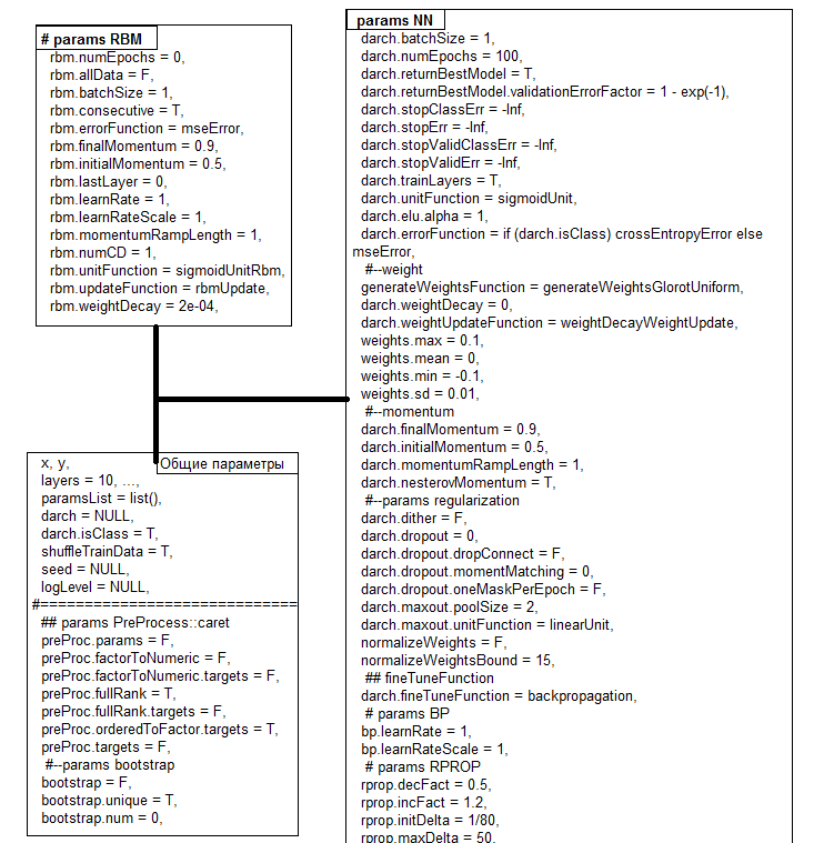
Fig.1. Structure of the DArch object
All parameters have a default values. These values are usually not optimal. All these parameters can be split into three groups - general, for RBM and for NN. We will consider some of them in detail later.
| Functions | Types |
|---|---|
| Initialization functions |
|
| Activation functions |
|
| Training functions |
|
| Level of training |
|
| Stabilization functions |
|
| Momentum |
|
| Stop conditions |
|
A deep neural network is made up of n RBM (n = layers -1) connected into an autoassociative network (SRBM) and the actual neural networks MLP with a number of layers. The layer-wise training of RBM is an unsupervised training on unlabeled data. Fine tuning of the neural network requires supervision and is carried out on labeled data.
Dividing these stages of training with parameters gives us an opportunity to use data of different volume (not different structure!!) and obtain several fine tuned models based on one pretraining. If data for pretraining and fine tuning are the same, training can be performed in one go without dividing it into two stages. Pretraining can be skipped (rbm.numEpochs = 0; darch.numEpochs = 10)). In that case, you can use only a multi-layer neural network or train only RBM (rbm.numEpochs = 10; darch.numEpochs = 0). You will still have an access to all internal parameters.
The trained neural network can be trained further on new data as many times as required. This is possible only with a limited number of models. Structural diagram of a deep neural network initialized by complex restricted Boltzmann machines (DNRBM) is shown on Fig.2.
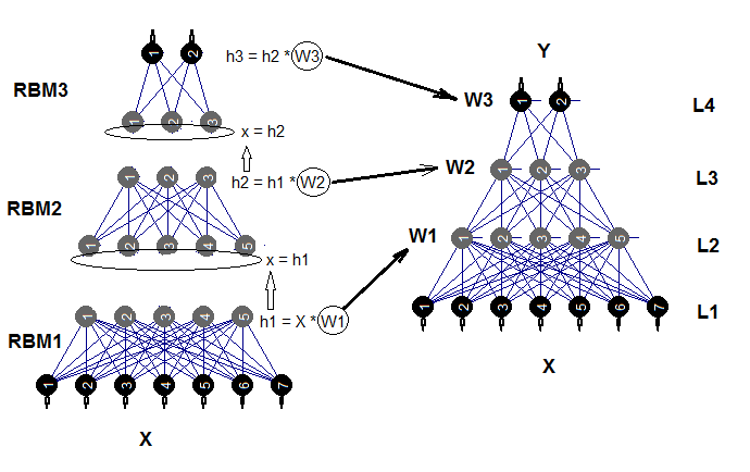
Fig.2. Structural diagram of DNSRBM
1.1. Initialization functions of neurons
There are two main initialization functions of neurons in the package.
- generateWeightsUniform() uses the runif(n, min, max) function and is implemented as follows:
> generateWeightsUniform
function (numUnits1, numUnits2, weights.min = getParameter(".weights.min",
    -0.1, ...), weights.max = getParameter(".weights.max", 0.1,
    ...), ...)
{
    matrix(runif(numUnits1 * numUnits2, weights.min, weights.max),
        nrow = numUnits1, ncol = numUnits2)
}
<environment: namespace:darch>
numUnits1 is the number of neurons on the previous layer and numUnits2 is the number of neurons on the current layer.
- generateWeightsNormal() uses the rnorm(n, mean, sd) function and is implemented in the package as follows:
> generateWeightsNormal
function (numUnits1, numUnits2, weights.mean = getParameter(".weights.mean",
    0, ...), weights.sd = getParameter(".weights.sd", 0.01, ...),
    ...)
{
    matrix(rnorm(numUnits1 * numUnits2, weights.mean, weights.sd),
        nrow = numUnits1, ncol = numUnits2)
}
<environment: namespace:darch>
Other four functions are using these two functions but define min, max, mean and sd with specific functions. You can study them if you enter the function name without brackets in the terminal.
1.2. Activation functions of neurons
Along with standard activation functions, the package suggests a wide range of new ones. Here are some of them:
x <- seq(-5, 5, 0.1)
par(mfrow = c(2,3))
plot(x, y = 1/(1 + exp(-x)), t = "l", main = "sigmoid")
abline(v = 0, col = 2)
plot(x, y = tanh(x), t = "l", main = "tanh")
abline(v = 0, h = 0, col = 2)
plot(x, y = log(1 + exp(x)), t = "l", main = "softplus");
abline(v = 0, col = 2)
plot(x, y = ifelse(x > 0, x ,exp(x) - 1), t = "l",
     main = "ELU")
abline(h = 0, v = 0, col = 2)
plot(x, y = ifelse(x > 0, x , 0), t = "l", main = "ReLU")
abline(h = 0, v = 0, col = 2)
par(mfrow = c(1,1))
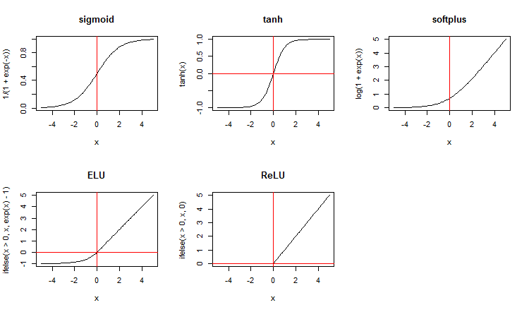
Fig.3. Activation functions of neurons
Let us consider the maxout activation function separately. This function comes from convoluted networks. The hidden layer of the neural network is divided by modules the size of the poolSize. The number of neurons in the hidden layer must be divisible by the size of the pool. For training, a neuron with a maximum activation is selected from the pool and sent to the input. The activation function of neurons in the pool is set separately. In simple words, this is a double layer (convoluted + maxpooling) with a limited capabilities in the filtration step. According to various publications, it produces good results together with dropout. Fig. 4. schematically shows a hidden layer with 8 neurons and two sizes of the pool
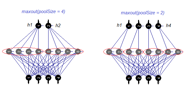
Fig.4. The maxout activation function
1.3. Training methods
Unfortunately, there are only two training methods in the package - backpropagation and rprop of the basic and improved version with weight updating during back-propagation and without. There is also a possibility to change the level of training with the help of the bp.learnRateScale. multiplier.
1.4. Methods of regulation and stabilization
- dropout is a dropout (zeroing the weight) of a part of neurons of the hidden layer during training. Neurons are zeroing in a random order. The relative number of neurons to be dropped out is defined by the darch.dropout parameter. The level of dropout in each hidden layer can be different. The dropout mask can be generated for each batch or for each epoch.
- dropconnect is turning off connections between a part of neurons of the current layer and the neurons of the previous layer. Connections are cut in a random order. The relative number of connections to be cut is defined by the same parameter darch.dropout (usually not greater than 0.5). According to some publications, dropconnect shows better results than dropout.
- dither is a way to prevent a retraining by dithering of the input data.
- weightDecay the weight of each neuron will be multiplied by (1 — weightDecay) before updating.
- normalizeWeights is a way to normalize an input vector of neuron weights with possible limitation from above (L2 norm)
The first three methods are only used separately.
1.5. Methods and parameters of training an RBM
Thee are two ways to train a SRBM. Either RBM is trained one at a time during rbm.numEpochs or each RBM is trained in turn one epoch at a time. The choice of one of these methods is made by the rbm.consecutive: parameter. TRUE or default is the first method and FALSE is the second method. Fig.5 presents a scheme of training in two variants. The rbm.lastLayer can be used to specify what layer of SRBM the pretraining should be stopped at. If 0, all layers are to be trained and if (-1) the upper layer is to be left untrained. This makes sense as the upper layer has to be trained separately and it takes much longer. Other parameters do not need additional explanations.
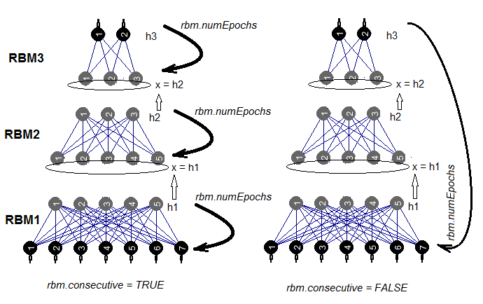
Fig.5. Two methods of training an SRBM
1.6. Methods and parameters of training a DNN
A DNN can be trained two ways - with pretraining and without it. Parameters used in these methods are totally different. For example, there is no point in using specific methods of initialization and regularization in training with pretraining. In fact, using these methods can make the result worse. The reason behind it is that after a pretraining, the weights of neurons in the hidden layers will be placed to the area close to optimal values and they will need only a minor fine tuning. To achieve the same result in training without pretraining, all available methods of initialization and regularization will have to be used. Usually, training a neural network this way takes longer.
So, we will focus on the training with pretraining. Normally, it happens in two stages.
- Training SRBM on a large set of unlabeled data. Pretraining parameters are set separately. As a result, we have a neural network initiated by weights of SRBM. Then the upper layer of the neural network is trained with labeled data with own training parameters. This way we have a neural network with a trained upper layer and initiated weights in the lower layers. Save it as an independent object for further use.
- At the second stage, we will use a few labeled samples, low level of training and a small number of training epochs for all the layers of neural network. This is a fine tuning of the network. The neural network is trained.
A possibility to divide stages of pretraining, fine tuning and further trainings gives incredible flexibility in creating training algorithms not only for one DNN but for training DNN committees. Fig.6. represents several variants of training DNN and DNN committees.
- Variant а. Save DNN in every n epochs during fine tuning. This way we will have a number of DNN with a different degree of training. Later, each of these neural networks can be used separately or as a part of a committee. The disadvantage of this scenario is that all DNN are trained on the same data as all of them had the same training parameters.
- Variant b. Fine tune the initiated DNN in parallel with different data sets (sliding window, growing window etc) and different parameters. As a result, we will have a DNN which will produce less correlated predictions than ones in variant а.
- Variant c Fine tune the initiated DNN sequentially with different data sets and different parameters. Save the intermediate models. This is what we earlier called further training. This can be performed each time when there is enough new data.
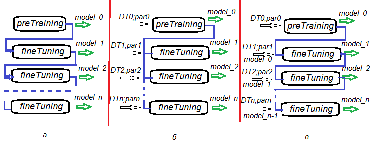
Fig.6. Variants of training a DNN
2. Testing the quality of work of a DNN depending on the parameters used.
2.1. Experiments
2.1.1. Input data (preparation)
We will use data and functions from the previous part of the article (1, 2, 3) . There we discussed in detail various variants of preliminary data preparation. I am going to briefly mention the stages of preliminary preparation that we are going to carry out. OHLCV is the initial data, same as before. Input data is digital filters and output data is ZigZag. Functions and the image of the work space Cotir.RData can be used.
The stages of preparing data to perform out will be gathered in separate functions:
- PrepareData() — create the initial dataSet and clean it from NA;
- SplitData() — divide the initial dataSet into the pretrain, train, val, test subsets;
- CappingData() — identify and impute outliers in all subsets.
To save the space in the article, I am not going to bring the listing of these functions here. They can be downloaded from GitHub as they have been considered in detail in previous articles. We are going to look into the results later. We are not going to discuss all methods of data transformation during the preliminary processing. Many of them are well known and widely used. We will use a less known method of discretization (supervised and unsupervised). In the second article we considered two packages of supervised discretization (discretization and smbinning). They contain different algorithms of discretization.
We will look into different methods of dividing continuous variables into bins and the ways to use these discretized variables in models.
What is binning?
Binning is a term used in scoring modeling. It is known as discretization in machine learning. This is a process of transforming a continuous variable into a finite number of intervals (bins). This helps to understand its distribution and relationship with the binary goal variable. Bins created in this process can become features of the predictive characteristic for use in models.
Why binning?
Despite some reservations about binning, it has significant advantages.
- It allows to include missing data (NA) and other specific calculations (dividing by zero, for instance) into the model.
- It controls or mitigates the impact of outliers on the model.
- It solves the problem of different scales in predictors making weighted coefficients comparable in the end model.
Unsupervised discretization
Unsupervised discretization divides a continuous function into bins without taking any other information into account. This division has two options. They are bins of equal length and bins of equal frequency.
| Option |
Aim |
Example |
Disadvantage |
|---|---|---|---|
| Bins of equal length |
Understand distribution of the variable |
Classical histogram with bunkers of the same length, which can be calculated using different rules (sturges, rice ets) |
The number of records in the bunker can be too small for a correct calculation |
| Bins of qual frequency |
Analyze the relationship with the binary goal variable using such indices as bad rate |
Quartilies or Percentiles | Selected cutoff points cannot maximize the difference between the bins at checking against the goal variable |
Supervised discretization
Supervised discretization divides the continuous variable into bins projected into the goal variable. The key idea here is to find such cutoff points that will maximize the difference between the groups.
Using such algorithms as ChiMerge or Recursive Partitioning, analysts can quickly find optimal points in seconds and evaluate their relationship with the goal variable using such indices as weight of evidence (WoE) and information value (IV).
WoE can be used as an instrument for transforming predictors at the stage of preprocessing for algorithms of supervised learning. During the discretization of predictors, we can substitute them with their new nominal variables or with the values of their WoE. The second variant is interesting because it allows to step away from transforming nominal variables (factors) into dummy ones. This gives a significant improvement in the quality of classification.
WOE and IV play two different roles in data analysis:
- WOE describes the relationship of the predictive variable and the binary goal variable.
- IV measures the strength of these relationships.
Let us figure out what WOE and IV are using diagrams and formulae. Let us recall the chart of the v.fatl variable split into 10 equifrequent areas from the second part of the article.
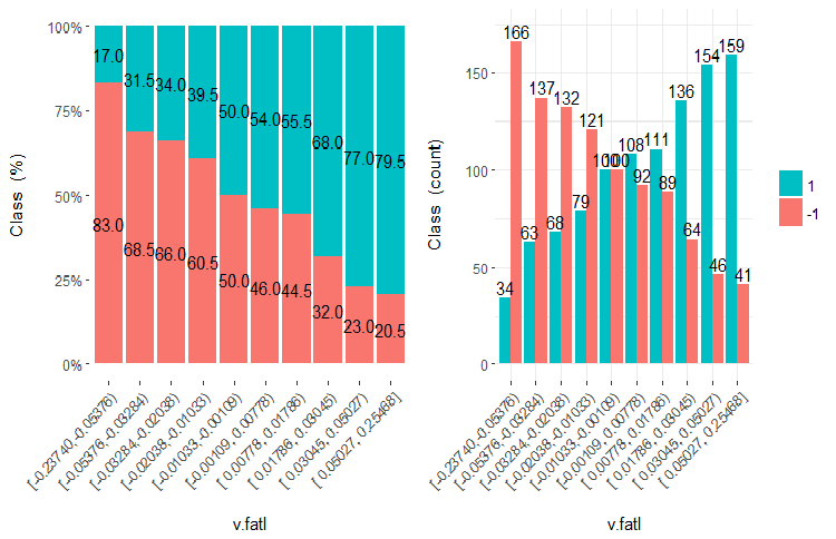
Fig.7. The v.fatl variable split into 10 equifrequent areas
Predictive capability of data (WOE)
As you can see, each bin has samples that get into the class "1" and class "-1". Predictive ability of the WoEi bins is calculated with the formula
WoEi = ln(Gi/Bi)*100
где:
Gi — relative frequency of "good" (in our case "good" = "1") samples in each bin of the variable;
Bi — relative frequency of "bad" (in our case "bad" = "-1") samples in each bin of the variable.
If WoEi = 1, which means that the number of "good" and "bad" samples in this bin is roughly the same, then the predictive ability of this bin is 0. If "good" samples outnumber "bad" ones, WOE >0 and vice versa.
Information value (IV)
This is the most common measure of identifying significance of variables and measuring the difference in the distribution of "good" and "bad" samples. Information value can be calculated with the formula:
IV = ∑ (Gi – Bi) ln (Gi/Bi)
The information value of a variable equals to the sum of all bins of the variable. The values of this coefficient could be interpreted as follows:
- below 0,02 — statistically insignificant variable;
- 0,02 – 0,1 — statistically weak variable;
- 0,1 – 0,3 — statistically significant variable;
- 0,3 and above — statistically strong variable.
Then, bins are merged/divided using various algorithms and optimization criteria to make the difference between these bins as big as possible. For example, the smbinning package uses Recursive Partitioning for categorization of numeric values and information value for working out optimal cutoff points. The discretization package solves this problem with ChiMerge and MDL. It should be kept in mind that cutoff points are obtained on the train set and used to divide the validation and test sets.
There are several packages that allow to make numeric variables discrete one way or another. They are discretization, smbinning, Information, InformationValue and woebinning. We need to make the test data set discreet, then divide the validation and test sets using this information. We also want to have visual control of the results. Because of these requirements, I chose the woebinning package.
The package automatically splits numeric values and factors and binds them to the binary goal variable. Here two approaches are catered for:
- implementation of fine and rough classification sequentially unites granulated classes and levels;
- a tree-like approach segments through iteration initial bins through binary splitting.
Both procedures merge divided bins based on the similar values of WOE and stop based on the IV criteria. Package can be used both with standalone variables or with the whole dataframe. This provides flexible tools for studying various solutions for binning and for their expanding on new data.
Let us do the calculation. We already have quotes from the terminal loaded into our work environment (or image of the work environment Cotir.RData from GitHub). Sequence of calculations and result:
- PrepareData() — create the initial data set dt[7906, 14], clean it from NA. The set includes the temporary label Data, input variables(12) and the goal variable Class (factor with two levels "-1" and "+1").
- SplitData() — divide initial data set dt[] into subsets pretrain, train, val, test in the ratio of 2000/1000/500/500, unite them into a dataframe DT[4, 4000, 14].
- CappingData() — identify and impute outliers in all subsets, get the DTcap[4, 4000, 14] set. Despite the fact that discretization is tolerant to outliers, we will impute them. You can experiment without this stage. As you can remember, parameters of outliers (pre.outl) are defined in the pretrain subset. Process the train/val/test sets using these parameters.
- NormData() — normalize the set, using the spatialSing method from the caret package. Similar to imputing outliers, parameters of normalization (preproc) are defined on the pretrain subset. Samples train/val/test are processed using these parameters. We have DTcap.n[4, 4000, 14] as a result.
- DiscretizeData() — define parameters of discretization (preCut), the quality of variables and their bins in the light of WOE and IV.
evalq({
  dt <- PrepareData(Data, Open, High, Low, Close, Volume)
  DT <- SplitData(dt, 2000, 1000, 500,500)
  pre.outl <- PreOutlier(DT$pretrain)
  DTcap <- CappingData(DT, impute = T, fill = T, dither = F,
                       pre.outl = pre.outl)
  preproc <- PreNorm(DTcap, meth = meth)
  DTcap.n <- NormData(DTcap, preproc = preproc)
  preCut <- PreDiscret(DTcap.n)
}, env)
Let us put the discretization data on all variables into a table and look at them:
evalq(tabulate.binning <- woe.binning.table(preCut), env)
> env$tabulate.binning
$`WOE Table for v.fatl`
          Final.Bin Total.Count Total.Distr. 0.Count 1.Count 0.Distr. 1.Distr. 1.Rate   WOE    IV
1  <= -0.3904381926         154         7.7%     130      24    13.2%     2.4%  15.6% 171.3 0.185
2 <= -0.03713814085         769        38.5%     498     271    50.4%    26.8%  35.2%  63.2 0.149
3   <= 0.1130198981         308        15.4%     141     167    14.3%    16.5%  54.2% -14.5 0.003
4            <= Inf         769        38.5%     219     550    22.2%    54.3%  71.5% -89.7 0.289
6             Total        2000       100.0%     988    1012   100.0%   100.0%  50.6%    NA 0.626

$`WOE Table for ftlm`
          Final.Bin Total.Count Total.Distr. 0.Count 1.Count 0.Distr. 1.Distr. 1.Rate   WOE    IV
1  <= -0.2344708291         462        23.1%     333     129    33.7%    12.7%  27.9%  97.2 0.204
2 <= -0.01368798447         461        23.1%     268     193    27.1%    19.1%  41.9%  35.2 0.028
3   <= 0.1789073635         461        23.1%     210     251    21.3%    24.8%  54.4% -15.4 0.005
4            <= Inf         616        30.8%     177     439    17.9%    43.4%  71.3% -88.4 0.225
6             Total        2000       100.0%     988    1012   100.0%   100.0%  50.6%    NA 0.463

$`WOE Table for rbci`
          Final.Bin Total.Count Total.Distr. 0.Count 1.Count 0.Distr. 1.Distr. 1.Rate   WOE    IV
1  <= -0.1718377948         616        30.8%     421     195    42.6%    19.3%  31.7%  79.4 0.185
2 <= -0.09060410462         153         7.6%      86      67     8.7%     6.6%  43.8%  27.4 0.006
3   <= 0.3208178176         923        46.2%     391     532    39.6%    52.6%  57.6% -28.4 0.037
4            <= Inf         308        15.4%      90     218     9.1%    21.5%  70.8% -86.1 0.107
6             Total        2000       100.0%     988    1012   100.0%   100.0%  50.6%    NA 0.335

$`WOE Table for v.rbci`
         Final.Bin Total.Count Total.Distr. 0.Count 1.Count 0.Distr. 1.Distr. 1.Rate   WOE    IV
1 <= -0.1837437563         616        30.8%     406     210    41.1%    20.8%  34.1%  68.3 0.139
2 <= 0.03581374495         461        23.1%     253     208    25.6%    20.6%  45.1%  22.0 0.011
3  <= 0.2503922644         461        23.1%     194     267    19.6%    26.4%  57.9% -29.5 0.020
4           <= Inf         462        23.1%     135     327    13.7%    32.3%  70.8% -86.1 0.161
6            Total        2000       100.0%     988    1012   100.0%   100.0%  50.6%    NA 0.331

$`WOE Table for v.satl`
          Final.Bin Total.Count Total.Distr. 0.Count 1.Count 0.Distr. 1.Distr. 1.Rate    WOE    IV
1 <= -0.01840058612         923        46.2%     585     338    59.2%    33.4%  36.6%   57.3 0.148
2   <= 0.3247097195         769        38.5%     316     453    32.0%    44.8%  58.9%  -33.6 0.043
3   <= 0.4003869443         154         7.7%      32     122     3.2%    12.1%  79.2% -131.4 0.116
4            <= Inf         154         7.7%      55      99     5.6%     9.8%  64.3%  -56.4 0.024
6             Total        2000       100.0%     988    1012   100.0%   100.0%  50.6%     NA 0.330

$`WOE Table for v.stlm`
         Final.Bin Total.Count Total.Distr. 0.Count 1.Count 0.Distr. 1.Distr. 1.Rate   WOE    IV
1 <= -0.4030051922         154         7.7%     118      36    11.9%     3.6%  23.4% 121.1 0.102
2 <= -0.1867821117         462        23.1%     282     180    28.5%    17.8%  39.0%  47.3 0.051
3  <= 0.1141896118         615        30.8%     301     314    30.5%    31.0%  51.1%  -1.8 0.000
4           <= Inf         769        38.5%     287     482    29.0%    47.6%  62.7% -49.4 0.092
6            Total        2000       100.0%     988    1012   100.0%   100.0%  50.6%    NA 0.244

$`WOE Table for pcci`
          Final.Bin Total.Count Total.Distr. 0.Count 1.Count 0.Distr. 1.Distr. 1.Rate   WOE    IV
1  <= -0.1738420887         616        30.8%     397     219    40.2%    21.6%  35.6%  61.9 0.115
2 <= -0.03163945242         307        15.3%     165     142    16.7%    14.0%  46.3%  17.4 0.005
3   <= 0.2553612644         615        30.8%     270     345    27.3%    34.1%  56.1% -22.1 0.015
4            <= Inf         462        23.1%     156     306    15.8%    30.2%  66.2% -65.0 0.094
6             Total        2000       100.0%     988    1012   100.0%   100.0%  50.6%    NA 0.228

$`WOE Table for v.ftlm`
          Final.Bin Total.Count Total.Distr. 0.Count 1.Count 0.Distr. 1.Distr. 1.Rate   WOE    IV
1 <= -0.03697698898         923        46.2%     555     368    56.2%    36.4%  39.9%  43.5 0.086
2   <= 0.2437475615         615        30.8%     279     336    28.2%    33.2%  54.6% -16.2 0.008
3            <= Inf         462        23.1%     154     308    15.6%    30.4%  66.7% -66.9 0.099
5             Total        2000       100.0%     988    1012   100.0%   100.0%  50.6%    NA 0.194

$`WOE Table for v.rftl`
         Final.Bin Total.Count Total.Distr. 0.Count 1.Count 0.Distr. 1.Distr. 1.Rate   WOE    IV
1 <= -0.1578370554         616        30.8%     372     244    37.7%    24.1%  39.6%  44.6 0.060
2  <= 0.1880959621         768        38.4%     384     384    38.9%    37.9%  50.0%   2.4 0.000
3  <= 0.3289762494         308        15.4%     129     179    13.1%    17.7%  58.1% -30.4 0.014
4           <= Inf         308        15.4%     103     205    10.4%    20.3%  66.6% -66.4 0.065
6            Total        2000       100.0%     988    1012   100.0%   100.0%  50.6%    NA 0.140

$`WOE Table for stlm`
         Final.Bin Total.Count Total.Distr. 0.Count 1.Count 0.Distr. 1.Distr. 1.Rate   WOE    IV
1 <= -0.4586732186         154         7.7%      60      94     6.1%     9.3%  61.0% -42.5 0.014
2 <= -0.1688696056         462        23.1%     266     196    26.9%    19.4%  42.4%  32.9 0.025
3  <= 0.2631157075         922        46.1%     440     482    44.5%    47.6%  52.3%  -6.7 0.002
4  <= 0.3592235072         154         7.7%      97      57     9.8%     5.6%  37.0%  55.6 0.023
5  <= 0.4846279843         154         7.7%      81      73     8.2%     7.2%  47.4%  12.8 0.001
6           <= Inf         154         7.7%      44     110     4.5%    10.9%  71.4% -89.2 0.057
8            Total        2000       100.0%     988    1012   100.0%   100.0%  50.6%    NA 0.122

$`WOE Table for v.rstl`
          Final.Bin Total.Count Total.Distr. 0.Count 1.Count 0.Distr. 1.Distr. 1.Rate   WOE    IV
1  <= -0.4541701981         154         7.7%      94      60     9.5%     5.9%  39.0%  47.3 0.017
2  <= -0.3526306487         154         7.7%      62      92     6.3%     9.1%  59.7% -37.1 0.010
3  <= -0.2496412214         154         7.7%      53     101     5.4%    10.0%  65.6% -62.1 0.029
4 <= -0.08554320418         307        15.3%     142     165    14.4%    16.3%  53.7% -12.6 0.002
5    <= 0.360854678         923        46.2%     491     432    49.7%    42.7%  46.8%  15.2 0.011
6            <= Inf         308        15.4%     146     162    14.8%    16.0%  52.6%  -8.0 0.001
8             Total        2000       100.0%     988    1012   100.0%   100.0%  50.6%    NA 0.070

$`WOE Table for v.pcci`
          Final.Bin Total.Count Total.Distr. 0.Count 1.Count 0.Distr. 1.Distr. 1.Rate   WOE    IV
1  <= -0.4410911486         154         7.7%      92      62     9.3%     6.1%  40.3%  41.9 0.013
2 <= -0.03637567714         769        38.5%     400     369    40.5%    36.5%  48.0%  10.5 0.004
3   <= 0.1801156117         461        23.1%     206     255    20.9%    25.2%  55.3% -18.9 0.008
4   <= 0.2480148615         154         7.7%      84      70     8.5%     6.9%  45.5%  20.6 0.003
5   <= 0.3348752487         154         7.7%      67      87     6.8%     8.6%  56.5% -23.7 0.004
6   <= 0.4397404288         154         7.7%      76      78     7.7%     7.7%  50.6%  -0.2 0.000
7            <= Inf         154         7.7%      63      91     6.4%     9.0%  59.1% -34.4 0.009
9             Total        2000       100.0%     988    1012   100.0%   100.0%  50.6%    NA 0.042
The table has the following values for each variable:
- Final.Bin — bin boundaries;
- Total.Count — total number of samples in the bin;
- Total.Distr — relative number of samples in the bin;
- 0.Count — number of samples belonging to the class "0";
- 1.Count — number of samples belonging to the class "1";
- 0.Distr — — relative number of samples belonging to the class "0";
- 1.Distr — relative number of samples belonging to the class "1";
- 1.Rate — percentage ratio of the samples of the class "1" to the number of samples of the class "0";
- WOE — predictive ability of the bins;
- IV — statistical importance of bins.
Graphic representation will be more illustrative. Plot the WOE charts of all variables in the increasing order of their IV based on this table:
> evalq(woe.binning.plot(preCut), env)
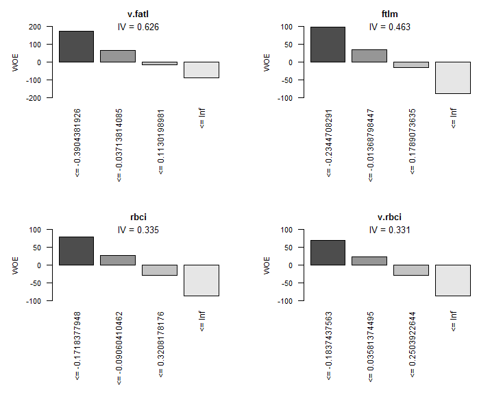
Fig.8. WOE of 4 best variables
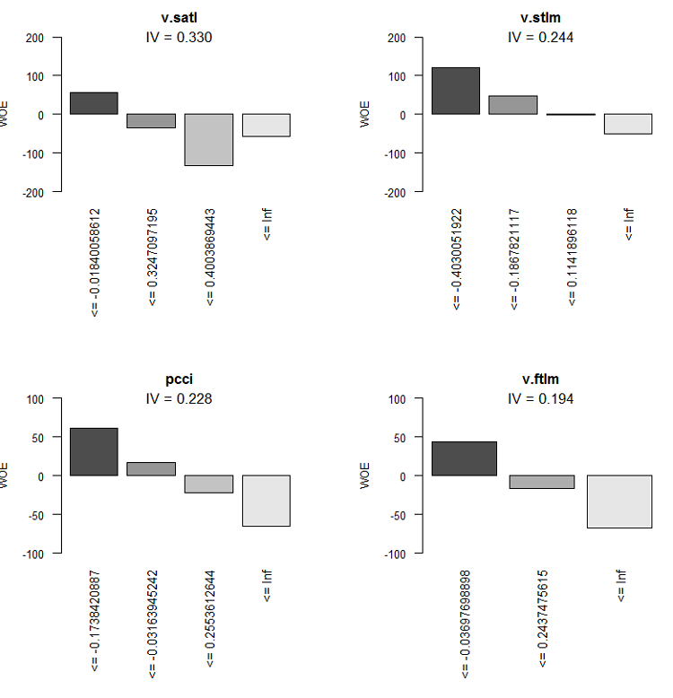
Fig.9. WOE of variables 5-8
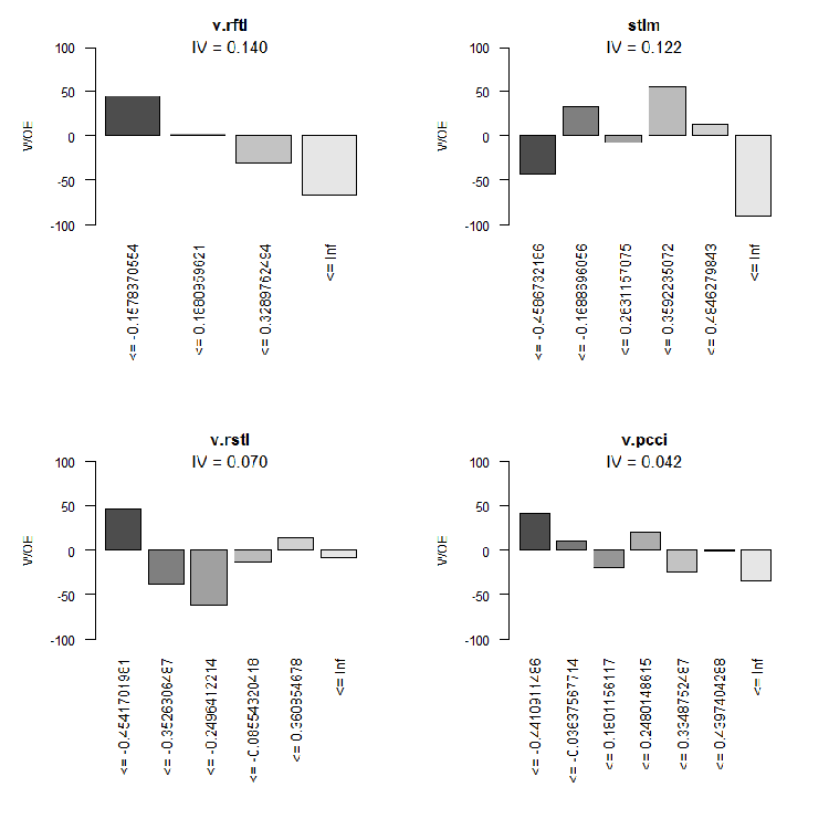
Fig.10. WOE of input variables 9-12
Chart of total ranging of variables by their IV.
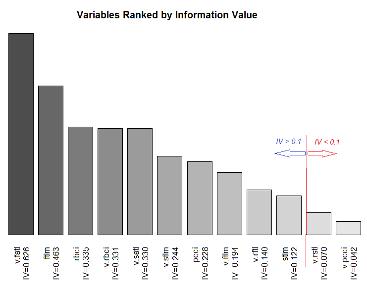
Fig.11. Ranging variables by their IV
We are not going to use two insignificant variables v.rstl and v.pcci, which have IV < 0.1. We can see from the charts that out of 10 significant variables, only v.satl and stlm have a nonlinear relationship with the goal variable. Other variables have a linear relationship.
For further experiments we need to create three sets. They are:
- DTbin is a data set where continuous numeric predictors are transformed into factors with the number of levels equal to the number of bins they are split into;
- DTdum is a data set where factor predictors of the DTbin data set are transformed into dummy binary variables;
- DTwoe is a data set where factor predictors are transformed into numeric variables by substituting their levels with the WOE values of these levels.
The first set DTbin is needed for training and obtaining metrics of the basic model. The second and the third sets will be used for the training of DNN and for comparing the efficiency of these two transformation methods.
The woe.binning.deploy() function of the woebinning package will enable us to solve this problem relatively easily. The following data has to be passed to the function:
- dataframe with predictors and the goal variable, where the goal variable must have the value of 0 or 1;
- parameters of discretization, obtained at the previous stage (preCut);
- names of variables that have to be categorized. If all variables have to be categorized, then just specify the name of the dataframe;
- specify the minimal IV for the variables not to be categorized;
- specify what additional variables (except categorized ones) we want to obtain. There are two variants - "woe" and "dum".
The function returns a dataframe containing initial variables, categorized variables and additional variables (if they were specified). The names of newly created variables are created by adding a corresponding prefix or suffix to the name of the initial variable. This way, the prefixes of all additional variables are "dum" or "woe" and categorized variables have the suffix "binned". Let us write a function DiscretizeData(), which will transform the initial data set using woe.binning.deploy().
DiscretizeData <- function(X, preCut, var){
  require(foreach)
  require(woeBinning)
  DTd <- list()
  foreach(i = 1:length(X)) %do% {
    X[[i]] %>% select(-Data) %>% targ.int() %>%
    woe.binning.deploy(preCut, min.iv.total = 0.1,
                       add.woe.or.dum.var = var) -> res
    return(res)
  } -> DTd
  list(pretrain = DTd[[1]] ,
       train = DTd[[2]] ,
       val =   DTd[[3]] ,
       test =  DTd[[4]] ) -> DTd
  return(DTd)
}
Input parameters of the function are initial data (list X) with the pretrain/train/val/test slots, parameters of discretization preCut and the type of the additional variable (string var).
The function will remove the "Data" variable from each slot and change the goal variable - factor "Class" for the numeric goal variable "Cl". Based on this, it will send woe.binning.deploy() to the input of the function. We will additionally specify in the entry parameters of this function the minimal IV = 0.1 for including the variables into the output set. At the output, we will receive a list with the same slots pretrain/train/val/test. In each slot, categorized variables and, if requested, additional variables will be added to the initial variables. Let us calculate all required sets and add raw data from the DTcap.n set to them.
evalq({
  require(dplyr)
  require(foreach)
    DTbin = DiscretizeData(DTcap.n, preCut = preCut, var = "")
    DTwoe = DiscretizeData(DTcap.n, preCut = preCut, var = "woe")
    DTdum = DiscretizeData(DTcap.n, preCut = preCut, var = "dum")
    X.woe <- list()
    X.bin <- list()
    X.dum <- list()
    foreach(i = 1:length(DTcap.n)) %do% {
      DTbin[[i]] %>% select(contains("binned")) -> X.bin[[i]]
      DTdum[[i]] %>% select(starts_with("dum")) -> X.dum[[i]]
      DTwoe[[i]] %>% select(starts_with("woe")) %>%
        divide_by(100) -> X.woe[[i]]
      return(list(bin =  X.bin[[i]], woe = X.woe[[i]],
                  dum = X.dum[[i]], raw = DTcap.n[[i]]))
    } -> DTcut
    list(pretrain = DTcut[[1]],
            train = DTcut[[2]],
              val =   DTcut[[3]],
             test =  DTcut[[4]] ) -> DTcut
    rm(DTwoe, DTdum, X.woe, X.bin, X.dum)
},
env)
Since WOE is a percentage value, we can divide the WOE by 100 and obtain values of variables that can be sent to the inputs of the neural network without additional normalization. Let us look at the structure of the obtained slot, for instance DTcut$val.
> env$DTcut$val %>% str()
List of 4
 $ bin:'data.frame':    501 obs. of  10 variables:
  ..$ v.fatl.binned: Factor w/ 5 levels "(-Inf,-0.3904381926]",..: 1 1 3 2 4 3 4 4 4 4 ...
  ..$ ftlm.binned  : Factor w/ 5 levels "(-Inf,-0.2344708291]",..: 2 1 1 1 2 2 3 4 4 4 ...
  ..$ rbci.binned  : Factor w/ 5 levels "(-Inf,-0.1718377948]",..: 2 1 2 1 2 3 3 3 4 4 ...
  ..$ v.rbci.binned: Factor w/ 5 levels "(-Inf,-0.1837437563]",..: 1 1 3 2 4 3 4 4 4 4 ...
  ..$ v.satl.binned: Factor w/ 5 levels "(-Inf,-0.01840058612]",..: 1 1 1 1 1 1 1 1 1 2 ...
  ..$ v.stlm.binned: Factor w/ 5 levels "(-Inf,-0.4030051922]",..: 2 2 3 2 3 2 3 3 4 4 ...
  ..$ pcci.binned  : Factor w/ 5 levels "(-Inf,-0.1738420887]",..: 1 1 4 2 4 2 4 2 2 3 ...
  ..$ v.ftlm.binned: Factor w/ 4 levels "(-Inf,-0.03697698898]",..: 1 1 3 2 3 2 3 3 2 2 ...
  ..$ v.rftl.binned: Factor w/ 5 levels "(-Inf,-0.1578370554]",..: 2 1 1 1 1 1 1 2 2 2 ...
  ..$ stlm.binned  : Factor w/ 7 levels "(-Inf,-0.4586732186]",..: 2 2 2 2 1 1 1 1 1 2 ...
 $ woe:'data.frame':    501 obs. of  10 variables:
  ..$ woe.v.fatl.binned: num [1:501] 1.713 1.713 -0.145 0.632 -0.897 ...
  ..$ woe.ftlm.binned  : num [1:501] 0.352 0.972 0.972 0.972 0.352 ...
  ..$ woe.rbci.binned  : num [1:501] 0.274 0.794 0.274 0.794 0.274 ...
  ..$ woe.v.rbci.binned: num [1:501] 0.683 0.683 -0.295 0.22 -0.861 ...
  ..$ woe.v.satl.binned: num [1:501] 0.573 0.573 0.573 0.573 0.573 ...
  ..$ woe.v.stlm.binned: num [1:501] 0.473 0.473 -0.0183 0.473 -0.0183 ...
  ..$ woe.pcci.binned  : num [1:501] 0.619 0.619 -0.65 0.174 -0.65 ...
  ..$ woe.v.ftlm.binned: num [1:501] 0.435 0.435 -0.669 -0.162 -0.669 ...
  ..$ woe.v.rftl.binned: num [1:501] 0.024 0.446 0.446 0.446 0.446 ...
  ..$ woe.stlm.binned  : num [1:501] 0.329 0.329 0.329 0.329 -0.425 ...
 $ dum:'data.frame':    501 obs. of  41 variables:
  ..$ dum.v.fatl.-Inf.-0.3904381926.binned          : num [1:501] 0 0 0 0 0 0 0 0 0 0 ...
  ..$ dum.v.fatl.-0.03713814085.0.1130198981.binned : num [1:501] 0 0 0 0 0 0 0 0 0 0 ...
  ..$ dum.v.fatl.-0.3904381926.-0.03713814085.binned: num [1:501] 0 0 0 0 0 0 0 0 0 0 ...
  ..$ dum.v.fatl.0.1130198981.Inf.binned            : num [1:501] 0 0 0 0 0 0 0 0 0 0 ...
  ..$ dum.ftlm.-0.2344708291.-0.01368798447.binned  : num [1:501] 0 0 0 0 0 0 0 0 0 0 ...
  ..$ dum.ftlm.-Inf.-0.2344708291.binned            : num [1:501] 0 0 0 0 0 0 0 0 0 0 ...
  ..$ dum.ftlm.-0.01368798447.0.1789073635.binned   : num [1:501] 0 0 0 0 0 0 0 0 0 0 ...
  ..$ dum.ftlm.0.1789073635.Inf.binned              : num [1:501] 0 0 0 0 0 0 0 0 0 0 ...
  .......................................................................................
  ..$ dum.stlm.-Inf.-0.4586732186.binned            : num [1:501] 0 0 0 0 0 0 0 0 0 0 ...
  ..$ dum.stlm.-0.1688696056.0.2631157075.binned    : num [1:501] 0 0 0 0 0 0 0 0 0 0 ...
  ..$ dum.stlm.0.2631157075.0.3592235072.binned     : num [1:501] 0 0 0 0 0 0 0 0 0 0 ...
  ..$ dum.stlm.0.3592235072.0.4846279843.binned     : num [1:501] 0 0 0 0 0 0 0 0 0 0 ...
  ..$ dum.stlm.0.4846279843.Inf.binned              : num [1:501] 0 0 0 0 0 0 0 0 0 0 ...
 $ raw:'data.frame':    501 obs. of  14 variables:
  ..$ Data  : POSIXct[1:501], format: "2017-02-23 15:30:00" "2017-02-23 15:45:00" ...
  ..$ ftlm  : num [1:501] -0.223 -0.374 -0.262 -0.31 -0.201 ...
  ..$ stlm  : num [1:501] -0.189 -0.257 -0.271 -0.389 -0.473 ...
  ..$ rbci  : num [1:501] -0.0945 -0.1925 -0.1348 -0.1801 -0.1192 ...
  ..$ pcci  : num [1:501] -0.5714 -0.2602 0.4459 -0.0478 0.2596 ...
  ..$ v.fatl: num [1:501] -0.426 -0.3977 0.0936 -0.1512 0.1178 ...
  ..$ v.satl: num [1:501] -0.35 -0.392 -0.177 -0.356 -0.316 ...
  ..$ v.rftl: num [1:501] -0.0547 -0.2065 -0.3253 -0.4185 -0.4589 ...
  ..$ v.rstl: num [1:501] 0.0153 -0.0273 -0.0636 -0.1281 -0.15 ...
  ..$ v.ftlm: num [1:501] -0.321 -0.217 0.253 0.101 0.345 ...
  ..$ v.stlm: num [1:501] -0.288 -0.3 -0.109 -0.219 -0.176 ...
  ..$ v.rbci: num [1:501] -0.2923 -0.2403 0.1909 0.0116 0.2868 ...
  ..$ v.pcci: num [1:501] -0.0298 0.3738 0.6153 -0.5643 0.2742 ...
  ..$ Class : Factor w/ 2 levels "-1","1": 1 1 1 1 2 2 2 2 2 1 ...
As you can see, the bin slot contains 10 factor variables with different number of levels. They have the suffix "binned". The woe slot contains 10 variables with factor levels changed for their WOE (they have the "woe" prefix). The dum slot has 41 numeric variables dummy with the values (0, 1) obtained from factor variables by coding one to one (have the prefix "dum"). There are 14 variables in the raw slot. They are Data — timestamp, Class — goal factor variable and 12 numeric predictors.
We have all the data that we will need for further experiments. The objects listed below should be in the environment env by now. Let us save the work area with these objects to the PartIV.RData file.
> ls(env)
 [1] "Close"    "Data"     "dt"       "DT"       "DTbin"    "DTcap"   "DTcap.n" "DTcut"  "High"
[10] "i"        "Low"      "Open"     "pre.outl" "preCut"   "preproc"  "Volume"
2.1.2. Basic model of comparison
We will use the OneR model implemented in the OneR package as the base model. This model is simple, reliable and easy to interpret. Information about the algorithm can be found in the package description. This model is working only with the bin data. The package contains auxiliary functions that can numeric variables discreet in different ways. As we have already transformed predictors into factors, we won't need them.
Now, I am going to elaborate the calculation shown below. Create the train/val/test sets by extracting correspondent slots from DTcut and adding the goal variable Class to them. We will train the model with the train set.
> evalq({
+   require(OneR)
+   require(dplyr)
+   require(magrittr)
+   train <- cbind(DTcut$train$bin, Class = DTcut$train$raw$Class) %>% as.data.frame()
+   val <- cbind(DTcut$val$bin, Class = DTcut$val$raw$Class) %>% as.data.frame()
+   test <- cbind(DTcut$test$bin, Class = DTcut$test$raw$Class) %>% as.data.frame()
+   model <- OneR(data = train, formula = NULL, ties.method = "chisq", #c("first","chisq"
+                 verbose = TRUE) #FALSE, TRUE
+ }, env)
Loading required package: OneR

    Attribute     Accuracy
1 * v.satl.binned 63.14%
2   v.fatl.binned 62.64%
3   ftlm.binned   62.54%
4   pcci.binned   61.44%
5   v.rftl.binned 59.74%
6   v.rbci.binned 58.94%
7   rbci.binned   58.64%
8   stlm.binned   58.04%
9   v.stlm.binned 57.54%
10  v.ftlm.binned 56.14%
---
Chosen attribute due to accuracy
and ties method (if applicable): '*'

Warning message:
In OneR(data = train, formula = NULL, ties.method = "chisq", verbose = TRUE) :
  data contains unused factor levels
The model selected the v.satl.binned variable with the basic accuracy of 63.14% as the basis for creating rules. Let us look at the general information about this model:
> summary(env$model)

Call:
OneR(data = train, formula = NULL, ties.method = "chisq", verbose = FALSE)

Rules:
If v.satl.binned = (-Inf,-0.01840058612]         then Class = -1
If v.satl.binned = (-0.01840058612,0.3247097195] then Class = 1
If v.satl.binned = (0.3247097195,0.4003869443]   then Class = 1
If v.satl.binned = (0.4003869443, Inf]           then Class = 1

Accuracy:
632 of 1001 instances classified correctly (63.14%)

Contingency table:
     v.satl.binned
Class (-Inf,-0.01840058612] (-0.01840058612,0.3247097195] (0.3247097195,0.4003869443] (0.4003869443, Inf]  Sum
  -1                  * 325                           161                          28                  37  551
  1                     143                         * 229                        * 35                * 43  450
  Sum                   468                           390                          63                  80 1001
---
Maximum in each column: '*'

Pearson's Chi-squared test:
X-squared = 74.429, df = 3, p-value = 4.803e-16
Graphic representation of the training result:
plot(env$model)
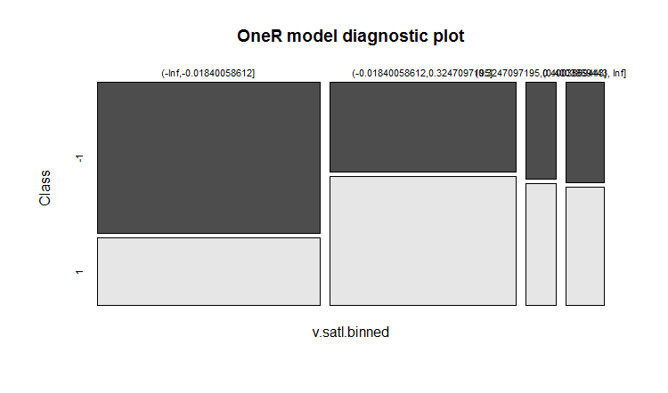
Fig.12. Distribution of the categories of the v.satl.binned variable by classes in the model
The accuracy of prediction during training is not very high. We are going to see what accuracy this model will show on the validation set:
> evalq(res.val <- eval_model(predict(model, val %>% as.data.frame()), val$Class),
+       env)

Confusion matrix (absolute):
          Actual
Prediction  -1   1 Sum
       -1  106  87 193
       1   100 208 308
       Sum 206 295 501

Confusion matrix (relative):
          Actual
Prediction   -1    1  Sum
       -1  0.21 0.17 0.39
       1   0.20 0.42 0.61
       Sum 0.41 0.59 1.00

Accuracy:
0.6267 (314/501)

Error rate:
0.3733 (187/501)

Error rate reduction (vs. base rate):
0.0922 (p-value = 0.04597)
and on the test set:
> evalq(res.test <- eval_model(predict(model, test %>% as.data.frame()), test$Class),
+       env)

Confusion matrix (absolute):
          Actual
Prediction  -1   1 Sum
       -1  130 102 232
       1    76 193 269
       Sum 206 295 501

Confusion matrix (relative):
          Actual
Prediction   -1    1  Sum
       -1  0.26 0.20 0.46
       1   0.15 0.39 0.54
       Sum 0.41 0.59 1.00

Accuracy:
0.6447 (323/501)

Error rate:
0.3553 (178/501)

Error rate reduction (vs. base rate):
0.1359 (p-value = 0.005976)
The results are not encouraging at all. Error rate reduction shows how accuracy has increased in relation to the base (0.5) level. Low value of p (< 0.05) indicates that this model is capable of producing predictions better than the basic level. Accuracy of the test set is 0.6447 (323/501), which is higher than the accuracy of the validation set. The test set is further away from the training set than the validation set. This result will be the reference point for comparing prediction results of our future models.
2.1.3. Structure of a DNN
We will use three data sets for training and testing:
- DTcut$$raw — 12 input variables (outliers imputed and normalized).
- DTcut$$dum — 41 binary variables.
- DTcut$$woe — 10 numeric variables.
We will use with all data sets the Class variable = factor with two levels. Structure of neural networks:
- DNNraw - layers = c(12, 16, 8(2), 2), activation functions c(tanh, maxout(lin), softmax)
- DNNwoe - layers = c(10, 16, 8(2), 2), activation functions c(tanh, maxout(lin), softmax)
- DNNdum - layers = c(41, 50, 8(2), 2), activation functions c(ReLU, maxout(ReLU), softmax)
The diagram below shows the structure of the DNNwoe neural network. Neural network has one input layer, two hidden layers and one output layer. Two other neural networks ( DNNdum, DNNraw) have a similar structure. They only differ in the number of neurons in layers and activation functions.
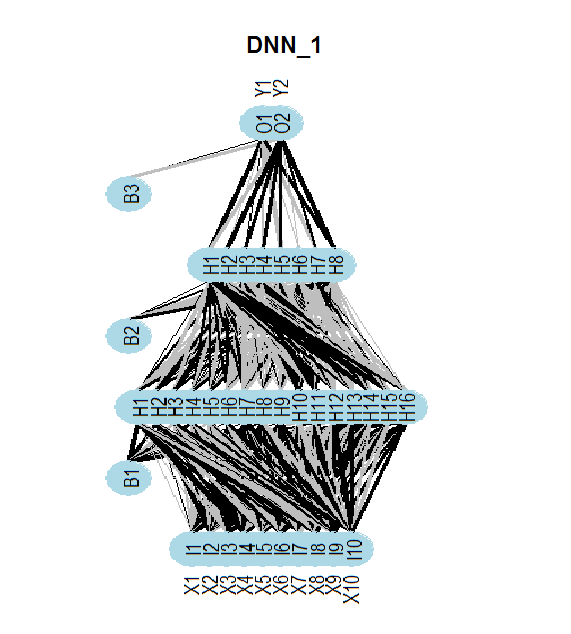
Fig.13. Structure of the neural network DNNwoe
2.1.4. Variants of training
With pretraining
Training will have two stages
- pretraining of SRBM with the /pretrain set followed by training only of the upper layer of the neural network, validation with the train set and parameters — par_0;
- fine tuning of the whole network with the train/val sets and parameters par_1.
We can save the intermediary models of fine tuning but it is not compulsory. The model that shows the best training results is to be saved. Parameters of these two stages should contain:
- par_0 — general parameters of the neural network, parameters of training of RBM and parameters of training of the upper layer of the DNN;
- par_1 — parameters of training of all layers of the DNN.
All parameters of DArch have default values. If we need different parameters at a certain stage of training, we can set them by a list and they will overwrite the default parameters. After the first stage of training, we will get the DArch structure with parameters and training results (training error, test error etc) and also the neural network initiated with the weights of the trained SRBM. To complete the second stage of training, you need to include the DArch structure obtained at the first stage into the list of parameters for this stage of training. Naturally, we will need a training and validation sets.
Let us consider parameters required for the first stage of training (pretraining of SRBM and training of the upper layer of neural network) and carry it out:
##=====CODE I etap===========================
evalq({
  require(darch)
  require(dplyr)
  require(magrittr)
  Ln <- c(0, 16, 8, 0)#     // the number of input and output neurons will be identified automatically from the data set
  nEp_0 <- 25
  #------------------
  par_0 <- list(
    layers = Ln, #         // let us take this parameter out of the list (for simplicity)
    seed = 54321,#         // if we want to obtain identical data during initialization
    logLevel = 5, #        // what level of information output we require
        # params RBM========================
        rbm.consecutive = F, # each RBM is trained one epoch at a time
    rbm.numEpochs = nEp_0,
    rbm.batchSize = 50,
    rbm.allData = TRUE,
    rbm.lastLayer = -1, #                       // do not train the upper layer of SRBM
    rbm.learnRate = 0.3,
    rbm.unitFunction = "tanhUnitRbm",
        # params NN ========================
    darch.batchSize = 50,
    darch.numEpochs = nEp_0,#                  // take this parameter out of the list for simplicity
    darch.trainLayers = c(F,F,T), #обучать     //upper layer only
    darch.unitFunction = c("tanhUnit","maxoutUnit", "softmaxUnit"),
    bp.learnRate = 0.5,
    bp.learnRateScale = 1,
    darch.weightDecay = 0.0002,
    darch.dither = F,
    darch.dropout = c(0.1,0.2,0.1),
    darch.fineTuneFunction = backpropagation, #rpropagation
    normalizeWeights = T,
    normalizeWeightsBound = 1,
    darch.weightUpdateFunction = c("weightDecayWeightUpdate",
                                   "maxoutWeightUpdate",
                                   "weightDecayWeightUpdate"),
    darch.dropout.oneMaskPerEpoch = T,
    darch.maxout.poolSize = 2,
    darch.maxout.unitFunction = "linearUnit")
#---------------------------

  DNN_default <- darch(darch = NULL,
                       paramsList = par_0,
                       x = DTcut$pretrain$woe %>% as.data.frame(),
                       y = DTcut$pretrain$raw$Class %>% as.data.frame(),
                       xValid = DTcut$train$woe %>% as.data.frame(),
                       yValid = DTcut$train$raw$Class %>% as.data.frame()
                       )
}, env)
Result upon completion of the first stage of training:
...........................

INFO [2017-09-11 14:12:19] Classification error on Train set (best model): 31.95% (639/2000)
INFO [2017-09-11 14:12:19] Train set (best model) Cross Entropy error: 1.233
INFO [2017-09-11 14:12:19] Classification error on Validation set (best model): 35.86% (359/1001)
INFO [2017-09-11 14:12:19] Validation set (best model) Cross Entropy error: 1.306
INFO [2017-09-11 14:12:19] Best model was found after epoch 3
INFO [2017-09-11 14:12:19] Final 0.632 validation Cross Entropy error: 1.279
INFO [2017-09-11 14:12:19] Final 0.632 validation classification error: 34.42%
INFO [2017-09-11 14:12:19] Fine-tuning finished after 5.975 secs
Second stage of training of neural network:
##=====CODE II etap===========================
evalq({
  require(darch)
  require(dplyr)
  require(magrittr)
  nEp_1 <- 100
  bp.learnRate <- 1
  par_1 <- list(
    layers = Ln,
    seed = 54321,
    logLevel = 5,
    rbm.numEpochs = 0,# SRBM is not to be trained!
    darch.batchSize = 50,
    darch.numEpochs = nEp_1,
    darch.trainLayers = c(T,T,T), #TRUE,
    darch.unitFunction = c("tanhUnit","maxoutUnit", "softmaxUnit"),
    bp.learnRate = bp.learnRate,
    bp.learnRateScale = 1,
    darch.weightDecay = 0.0002,
    darch.dither = F,
    darch.dropout = c(0.1,0.2,0.1),
    darch.fineTuneFunction = backpropagation, #rpropagation backpropagation
    normalizeWeights = T,
    normalizeWeightsBound = 1,
    darch.weightUpdateFunction = c("weightDecayWeightUpdate",
                                   "maxoutWeightUpdate",
                                   "weightDecayWeightUpdate"),
    darch.dropout.oneMaskPerEpoch = T,
    darch.maxout.poolSize = 2,
    darch.maxout.unitFunction = exponentialLinearUnit,
    darch.elu.alpha = 2)
        #------------------------------
        DNN_1 <- darch( darch = DNN_default, paramsList = par_1,
                 x = DTcut$train$woe %>% as.data.frame(),
                 y = DTcut$train$raw$Class %>% as.data.frame(),
                 xValid = DTcut$val$woe %>% as.data.frame(),
                 yValid = DTcut$val$raw$Class %>% as.data.frame()
                 )
}, env)
Result of the second stage of training:
...........................
INFO [2017-09-11 15:48:37] Finished epoch 100 of 100 after 0.279 secs (3666 patterns/sec)
INFO [2017-09-11 15:48:37] Classification error on Train set (best model): 31.97% (320/1001)
INFO [2017-09-11 15:48:37] Train set (best model) Cross Entropy error: 1.225
INFO [2017-09-11 15:48:37] Classification error on Validation set (best model): 31.14% (156/501)
INFO [2017-09-11 15:48:37] Validation set (best model) Cross Entropy error: 1.190
INFO [2017-09-11 15:48:37] Best model was found after epoch 96
INFO [2017-09-11 15:48:37] Final 0.632 validation Cross Entropy error: 1.203
INFO [2017-09-11 15:48:37] Final 0.632 validation classification error: 31.44%
INFO [2017-09-11 15:48:37] Fine-tuning finished after 37.22 secs
Chart of the prediction error change during the second stage of training:
plot(env$DNN_1, y = "raw")
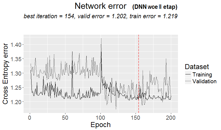
Fig.14. Changing of the classification error during the second stage of training
Let us take a look at the classification error of the final model on the test set:
#-----------
evalq({
  xValid = DTcut$test$woe %>% as.data.frame()
  yValid = DTcut$test$raw$Class %>% as.vector()
  Ypredict <- predict(DNN_1, newdata = xValid, type = "class")
  numIncorrect <- sum(Ypredict != yValid)
  cat(paste0("Incorrect classifications on all examples: ", numIncorrect, " (",
           round(numIncorrect/nrow(xValid)*100, 2), "%)\n"))
   caret::confusionMatrix(yValid, Ypredict)
}, env)
Incorrect classifications on all examples: 166 (33.13%)
Confusion Matrix and Statistics

          Reference
Prediction  -1   1
        -1 129  77
        1   89 206

               Accuracy : 0.6687
                 95% CI : (0.6255, 0.7098)
    No Information Rate : 0.5649
    P-Value [Acc > NIR] : 1.307e-06

                  Kappa : 0.3217
 Mcnemar's Test P-Value : 0.3932

            Sensitivity : 0.5917
            Specificity : 0.7279
         Pos Pred Value : 0.6262
         Neg Pred Value : 0.6983
             Prevalence : 0.4351
         Detection Rate : 0.2575
   Detection Prevalence : 0.4112
      Balanced Accuracy : 0.6598

       'Positive' Class : -1
#----------------------------------------
The accuracy on this data set (woe) with these parameters that are far from optimal, is much higher than the accuracy of the basic model. There is a significant potential to increase accuracy by optimizing hyperparameters of the DNN. If the calculation is repeated, data may not be exactly the same as in the article.
Let us bring our scripts to a more compact form for further calculations with other data sets. Let us write a function for the woe set:
#-------------------
DNN.train.woe <- function(param, X){
  require(darch)
  require(magrittr)
  darch( darch = NULL, paramsList = param[[1]],
         x = X[[1]]$woe %>% as.data.frame(),
         y = X[[1]]$raw$Class %>% as.data.frame(),
         xValid = X[[2]]$woe %>% as.data.frame(),
         yValid = X[[2]]$raw$Class %>% as.data.frame()
  ) %>%
    darch( ., paramsList = param[[2]],
           x = X[[2]]$woe %>% as.data.frame(),
           y = X[[2]]$raw$Class %>% as.data.frame(),
           xValid = X[[3]]$woe %>% as.data.frame(),
           yValid = X[[3]]$raw$Class %>% as.data.frame()
    ) -> Darch
  return(Darch)
}
Repeat the calculations for the DTcut$$woe data set in a compact form:
evalq({
  require(darch)
  require(magrittr)
  Ln <- c(0, 16, 8, 0)
  nEp_0 <- 25
  nEp_1 <- 25
  rbm.learnRate = c(0.5,0.3,0.1)
  bp.learnRate <- c(0.5,0.3,0.1)
  list(par_0, par_1) %>% DNN.train.woe(DTcut) -> Dnn.woe
  xValid = DTcut$test$woe %>% as.data.frame()
  yValid = DTcut$test$raw$Class %>% as.vector()
  Ypredict <- predict(Dnn.woe, newdata = xValid, type = "class")
  numIncorrect <- sum(Ypredict != yValid)
  cat(paste0("Incorrect classifications on all examples: ", numIncorrect, " (",
             round(numIncorrect/nrow(xValid)*100, 2), "%)\n"))
  caret::confusionMatrix(yValid, Ypredict) -> cM.woe
}, env)
Do the calculation for the DTcut$$raw data set:
#-------------------------
DNN.train.raw <- function(param, X){
  require(darch)
  require(magrittr)
  darch( darch = NULL, paramsList = param[[1]],
         x = X[[1]]$raw %>% tbl_df %>% select(-c(Data, Class)),
         y = X[[1]]$raw$Class %>% as.data.frame(),
         xValid = X[[2]]$raw %>% tbl_df %>% select(-c(Data, Class)),
         yValid = X[[2]]$raw$Class %>% as.data.frame()
  ) %>%
    darch( ., paramsList = param[[2]],
           x = X[[2]]$raw %>% tbl_df %>% select(-c(Data, Class)),
           y = X[[2]]$raw$Class %>% as.data.frame(),
           xValid = X[[3]]$raw %>% tbl_df %>% select(-c(Data, Class)),
           yValid = X[[3]]$raw$Class %>% as.data.frame()
    ) -> Darch
  return(Darch)
}
#-------------------------------
evalq({
  require(darch)
  require(magrittr)
  Ln <- c(0, 16, 8, 0)
  nEp_0 <- 25
  nEp_1 <- 25
  rbm.learnRate = c(0.5,0.3,0.1)
  bp.learnRate <- c(0.5,0.3,0.1)
  list(par_0, par_1) %>% DNN.train.raw(DTcut) -> Dnn.raw
  xValid = DTcut$test$raw %>% tbl_df %>% select(-c(Data, Class))
  yValid = DTcut$test$raw$Class %>% as.vector()
  Ypredict <- predict(Dnn.raw, newdata = xValid, type = "class")
  numIncorrect <- sum(Ypredict != yValid)
  cat(paste0("Incorrect classifications on all examples: ", numIncorrect, " (",
             round(numIncorrect/nrow(xValid)*100, 2), "%)\n"))
  caret::confusionMatrix(yValid, Ypredict) -> cM.raw
}, env)
#----------------------------
Below is the result and the chart of the classification error change for this set:
> env$cM.raw
Confusion Matrix and Statistics

          Reference
Prediction  -1   1
        -1 133  73
        1   86 209

               Accuracy : 0.6826
                 95% CI : (0.6399, 0.7232)
    No Information Rate : 0.5629
    P-Value [Acc > NIR] : 2.667e-08

                  Kappa : 0.3508
 Mcnemar's Test P-Value : 0.3413

            Sensitivity : 0.6073
            Specificity : 0.7411
         Pos Pred Value : 0.6456
         Neg Pred Value : 0.7085
             Prevalence : 0.4371
         Detection Rate : 0.2655
   Detection Prevalence : 0.4112
      Balanced Accuracy : 0.6742

       'Positive' Class : -1
#--------------------------------------
plot(env$Dnn.raw, y = "raw")
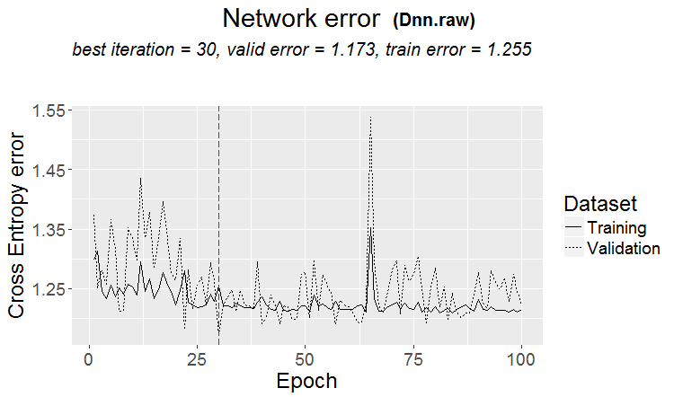
Fig.15. Classification error change at the second stage
I was not able to train the neural network with the DTcut$$dum data. You can try to do this yourself. For instance, input the DTcut$$bin data and arrange in the training parameters for predictors to be converted to dummy.
Training without pretraining
Let us train the neural network without pretraining with the same data (woe, raw) on the pretrain/train/val sets. Let us see the result.
#-------WOE----------------
evalq({
  require(darch)
  require(magrittr)
  Ln <- c(0, 16, 8, 0)
  nEp_1 <- 100
  bp.learnRate <- c(0.5,0.7,0.1)
  #--param----------------
  par_1 <- list(
    layers = Ln,
    seed = 54321,
    logLevel = 5,
    rbm.numEpochs = 0,# SRBM is not to be trained!
    darch.batchSize = 50,
    darch.numEpochs = nEp_1,
    darch.trainLayers = c(T,T,T), #TRUE,
    darch.unitFunction = c("tanhUnit","maxoutUnit", "softmaxUnit"),
    bp.learnRate = bp.learnRate,
    bp.learnRateScale = 1,
    darch.weightDecay = 0.0002,
    darch.dither = F,
    darch.dropout = c(0.0,0.2,0.1),
    darch.fineTuneFunction = backpropagation, #rpropagation backpropagation
    normalizeWeights = T,
    normalizeWeightsBound = 1,
    darch.weightUpdateFunction = c("weightDecayWeightUpdate",
                                   "maxoutWeightUpdate",
                                   "weightDecayWeightUpdate"),
    darch.dropout.oneMaskPerEpoch = T,
    darch.maxout.poolSize = 2,
    darch.maxout.unitFunction = exponentialLinearUnit,
    darch.elu.alpha = 2)
  #--train---------------------------
  darch( darch = NULL, paramsList = par_1,
         x = DTcut[[1]]$woe %>% as.data.frame(),
         y = DTcut[[1]]$raw$Class %>% as.data.frame(),
         xValid = DTcut[[2]]$woe %>% as.data.frame(),
         yValid = DTcut[[2]]$raw$Class %>% as.data.frame()
  ) -> Dnn.woe.I
  #---test--------------------------
  xValid = DTcut$val$woe %>% as.data.frame()
  yValid = DTcut$val$raw$Class %>% as.vector()
  Ypredict <- predict(Dnn.woe.I, newdata = xValid, type = "class")
  numIncorrect <- sum(Ypredict != yValid)
  cat(paste0("Incorrect classifications on all examples: ", numIncorrect, " (",
             round(numIncorrect/nrow(xValid)*100, 2), "%)\n"))
  caret::confusionMatrix(yValid, Ypredict) -> cM.woe.I
}, env)
#---------Ris16------------------------------------
plot(env$Dnn.woe.I, type = "class")
env$cM.woe.I
Metrics:
.......................................................
INFO [2017-09-14 10:38:01] Classification error on Train set (best model): 28.7% (574/2000)
INFO [2017-09-14 10:38:01] Train set (best model) Cross Entropy error: 1.140
INFO [2017-09-14 10:38:02] Classification error on Validation set (best model): 35.86% (359/1001)
INFO [2017-09-14 10:38:02] Validation set (best model) Cross Entropy error: 1.299
INFO [2017-09-14 10:38:02] Best model was found after epoch 67
INFO [2017-09-14 10:38:02] Final 0.632 validation Cross Entropy error: 1.241
INFO [2017-09-14 10:38:02] Final 0.632 validation classification error: 33.23%
INFO [2017-09-14 10:38:02] Fine-tuning finished after 37.13 secs
Incorrect classifications on all examples: 150 (29.94%)
> env$cM.woe.I
Confusion Matrix and Statistics

          Reference
Prediction  -1   1
        -1 144  62
        1   88 207

               Accuracy : 0.7006
                 95% CI : (0.6584, 0.7404)
    No Information Rate : 0.5369
    P-Value [Acc > NIR] : 5.393e-14

                  Kappa : 0.3932
 Mcnemar's Test P-Value : 0.04123

            Sensitivity : 0.6207
            Specificity : 0.7695
         Pos Pred Value : 0.6990
         Neg Pred Value : 0.7017
             Prevalence : 0.4631
         Detection Rate : 0.2874
   Detection Prevalence : 0.4112
      Balanced Accuracy : 0.6951

       'Positive' Class : -1
Chart of the classification error change during training:
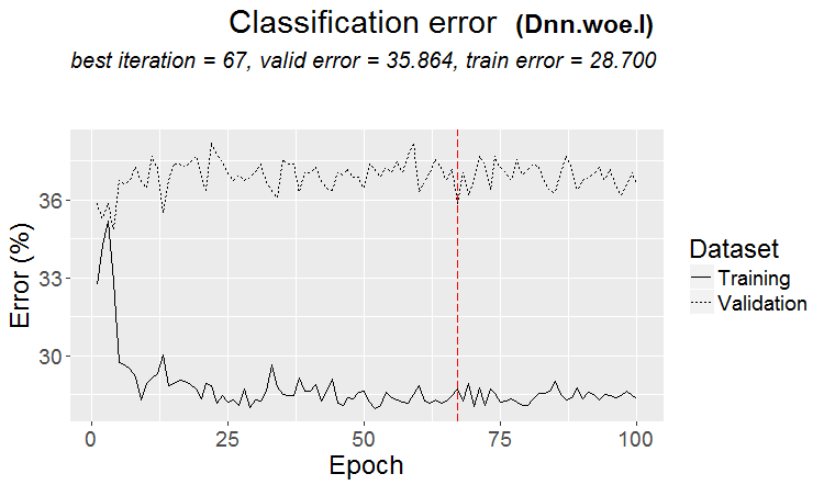
Fig.16. Classification error change without pretraining with the $woe set
Same for the set /raw:
evalq({
  require(darch)
  require(magrittr)
  Ln <- c(0, 16, 8, 0)
  nEp_1 <- 100
  bp.learnRate <- c(0.5,0.7,0.1)
  #--param-----------------------------
  par_1 <- list(
    layers = Ln,
    seed = 54321,
    logLevel = 5,
    rbm.numEpochs = 0,# SRBM is not to be trained!
    darch.batchSize = 50,
    darch.numEpochs = nEp_1,
    darch.trainLayers = c(T,T,T), #TRUE,
    darch.unitFunction = c("tanhUnit","maxoutUnit", "softmaxUnit"),
    bp.learnRate = bp.learnRate,
    bp.learnRateScale = 1,
    darch.weightDecay = 0.0002,
    darch.dither = F,
    darch.dropout = c(0.1,0.2,0.1),
    darch.fineTuneFunction = backpropagation, #rpropagation backpropagation
    normalizeWeights = T,
    normalizeWeightsBound = 1,
    darch.weightUpdateFunction = c("weightDecayWeightUpdate",
                                   "maxoutWeightUpdate",
                                   "weightDecayWeightUpdate"),
    darch.dropout.oneMaskPerEpoch = T,
    darch.maxout.poolSize = 2,
    darch.maxout.unitFunction = exponentialLinearUnit,
    darch.elu.alpha = 2)
  #---train------------------------------
  darch( darch = NULL, paramsList = par_1,
         x = DTcut[[1]]$raw %>% tbl_df %>% select(-c(Data, Class)) ,
         y = DTcut[[1]]$raw$Class %>% as.vector(),
         xValid = DTcut[[2]]$raw %>% tbl_df %>% select(-c(Data, Class)) ,
         yValid = DTcut[[2]]$raw$Class %>% as.vector()
  ) -> Dnn.raw.I
  #---test--------------------------------
  xValid = DTcut[[3]]$raw %>% tbl_df %>% select(-c(Data, Class))
  yValid = DTcut[[3]]$raw$Class %>% as.vector()
  Ypredict <- predict(Dnn.raw.I, newdata = xValid, type = "class")
  numIncorrect <- sum(Ypredict != yValid)
  cat(paste0("Incorrect classifications on all examples: ", numIncorrect, " (",
             round(numIncorrect/nrow(xValid)*100, 2), "%)\n"))
  caret::confusionMatrix(yValid, Ypredict) -> cM.raw.I
}, env)
#---------Ris17----------------------------------
env$cM.raw.I
plot(env$Dnn.raw.I, type = "class")
Metrics:
INFO [2017-09-14 11:06:13] Classification error on Train set (best model): 30.75% (615/2000)
INFO [2017-09-14 11:06:13] Train set (best model) Cross Entropy error: 1.189
INFO [2017-09-14 11:06:13] Classification error on Validation set (best model): 33.67% (337/1001)
INFO [2017-09-14 11:06:13] Validation set (best model) Cross Entropy error: 1.236
INFO [2017-09-14 11:06:13] Best model was found after epoch 45
INFO [2017-09-14 11:06:13] Final 0.632 validation Cross Entropy error: 1.219
INFO [2017-09-14 11:06:13] Final 0.632 validation classification error: 32.59%
INFO [2017-09-14 11:06:13] Fine-tuning finished after 35.47 secs
Incorrect classifications on all examples: 161 (32.14%)
> #---------Ris17----------------------------------
> env$cM.raw.I
Confusion Matrix and Statistics

          Reference
Prediction  -1   1
        -1 140  66
        1   95 200

               Accuracy : 0.6786
                 95% CI : (0.6358, 0.7194)
    No Information Rate : 0.5309
    P-Value [Acc > NIR] : 1.283e-11

                  Kappa : 0.3501
 Mcnemar's Test P-Value : 0.02733

            Sensitivity : 0.5957
            Specificity : 0.7519
         Pos Pred Value : 0.6796
         Neg Pred Value : 0.6780
             Prevalence : 0.4691
         Detection Rate : 0.2794
   Detection Prevalence : 0.4112
      Balanced Accuracy : 0.6738

       'Positive' Class : -1
Chart of the classification error change:
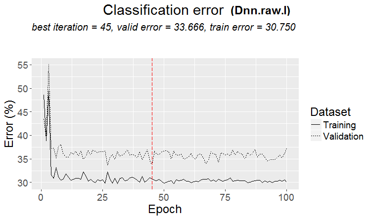
Fig.17. Change of the classification error without pretraining with the $raw set
2.2. Result analysis
Let us put the result of our experiments into a table:
| Type of training | Set /woe | Set /raw |
|---|---|---|
| With pretraining | 0.6687 (0.6255 - 0.7098) | 0.6826(0.6399 - 0.7232) |
| Without pretraining | 0.7006(0.6589 - 0.7404) | 0.6786(0.6359 - 0.7194) |
Classification error with pretraining is nearly the same in both sets. It is in the range of 30+/-4%. Despite a lower error, it is clear from the chart of the classification error change that there was a retraining during training without pretraining (the error on the validation and test sets is significantly greater than the training error). Therefore we will use training with pretraining in our further experiments.
The result is not much greater than the result of the basic model. We have a possibility to improve the characteristics by optimizing some hyperparameters. We will do this in the next article.
Conclusion
Despite the limitations (for example, only two basic training methods), the darch package allows to create neural networks different in structure and parameters. This package is a good tool for deep studying of neural networks.
Weak characteristics of the DNN is mainly explained by the use of the default parameters or parameters close to them. The woe set did not show any advantages before the raw set. Therefore in the next article we will:
- optimize a part of hyperparameters in DNN.woe created earlier;
- will create a DNN, using the TensorFlow library, test it and compare results with the DNN (darch);
- will create an ensemble of neural networks of different kind (bagging, stacking) and see how this improves the quality of predictions.
Application
GitHub/PartIV contains:
- FunPrepareData.R — functions used for preparing data
- RunPrepareData.R — scripts for preparing data
- Experiment.R — scripts for running experiments
- Part_IV.RData — image of the work area with all objects obtained after the stage of preparing data
- SessionInfo.txt — information about used software
- Darch_default.txt — list of parameters of the DArch structure with default values
Translated from Russian by MetaQuotes Ltd.
Original article: https://www.mql5.com/ru/articles/3473
Warning: All rights to these materials are reserved by MetaQuotes Ltd. Copying or reprinting of these materials in whole or in part is prohibited.
This article was written by a user of the site and reflects their personal views. MetaQuotes Ltd is not responsible for the accuracy of the information presented, nor for any consequences resulting from the use of the solutions, strategies or recommendations described.
 TradeObjects: Automation of trading based on MetaTrader graphical objects
 Cross-Platform Expert Advisor: Custom Stops, Breakeven and Trailing
 Risk Evaluation in the Sequence of Deals with One Asset
 Deep Neural Networks (Part III). Sample selection and dimensionality reduction
- Free trading apps
- Over 8,000 signals for copying
- Economic news for exploring financial markets
You agree to website policy and terms of use
Благодарим вас за использование моего пакета OneR. Еще раз увлекательно видеть, что даже сложный DNN не намного лучше, чем модель OneR!
This is only true for DNN with default parameters. With optimized hyperparameters, DNN shows much better results. See Part V.
Good luck
This is only true for DNN with default parameters. With optimized hyperparameters, DNN shows much better results. See Part V.
Good luck
Did you get a trade result?
Everyone's back to the mash. That's another topic.