
Deep Neural Networks (Part VI). Ensemble of neural network classifiers: bagging

Contents
- Introduction
- Ensembles of neural network classifiers
- bagging
- Generating the source data sets
- Arranging predictors by information importance
- Creating, training and testing the ensemble of classifiers
- Combining individual outputs of classifiers (averaging/voting)
- Ensemble pruning and its methods
- Optimizing hyperparameters of ensemble members. Features and methods
- Training and testing the ensemble with optimal hyperparameters
- Conclusion
- Attachments
Introduction
The previous article of this series discussed hyperparameters of the DNN model, trained it with several examples, and tested it. The quality of the resulting model was quite high.
We also discussed the possibilities of how to improve the classification quality. One of them is to use an ensemble of neural networks. This variant of amplification will be discussed in this article.
1. Ensembles of neural network classifiers
Studies show that classifier ensembles are usually more accurate than individual classifiers. One such ensemble is shown in Figure 1a. It uses several classifiers, with each of them making a decision about the object fed as input. Then these individual decisions are aggregated in a combiner. The ensemble outputs a class label for the object.
It is intuitive that the ensemble of classifiers cannot be strictly defined. This general uncertainty is illustrated in Figure 1b-d. In essence, any ensemble is a classifier itself (Figure 1b). The base classifiers comprising it will extract complex functions of (often implicit) regularities, and the combiner will become a simple classifier aggregating these functions.
On the other hand, nothing prevents us from calling a conventional standard neural network classifier an ensemble (Figure 1c). Neurons on its penultimate layer can be considered as separate classifiers. Their decisions must be "deciphered" in the combiner, whose role is played by the top layer.
And finally, the functions can be considered as primitive classifiers, and the classifier as their complex combiner (Figure 1d).
We combine simple trainable classifiers to obtain an accurate decision on classification. But is this the right way to go?
In her critical review article "Multiple Classifier Combination: Lessons and Next steps", published in 2002, Tin Kam Ho wrote:
"Instead of looking for the best set of features and the best classifier, now we look for the best set of classifiers and then the best combination method. One can imagine that very soon we will be looking for the best set of combination methods and then the best way to use them all. If we do not take the chance to review the fundamental problems arising from this challenge, we are bound to be driven into such an infinite recurrence, dragging along more and more complicated combination schemes and theories, and gradually losing sight of the original problem."

Fig.1. What is an ensemble of classifiers?
The lesson is that we have to find the optimal way to use existing tools and methods before creating new complex projects.
It is known that classifiers of neural networks are "universal approximants". This means that any classification boundary, no matter its complexity, can be approximated by a finite neural network with any required accuracy. However, this knowledge does not give us a way to create or train such a network. The idea of combining classifiers is an attempt to solve the problem by composing a network of managed building blocks.
Methods of composing an ensemble are meta algorithms that combine several machine learning methods into one predictive model, in order to:
- reduce variance — bagging;
- reduce bias — boosting;
- improve predictions — stacking.
These methods can be divided into two groups:
- parallel methods of constructing an ensemble, where the base models are generated in parallel (for example, a random forest). The idea is to use the independency between the base models and to reduce the error by averaging. Hence, the main requirement for models — low mutual correlation and high diversity.
- sequential ensemble methods, where the base models are generated sequentially (for example, AdaBoost, XGBoost). The main idea here is to use the dependency between the base models. Here, the overall quality can be increased by assigning higher weights to examples that were previously incorrectly classified.
Most ensemble methods use a single base learning algorithm when creating homogeneous base models. This leads to homogeneous ensembles. There are also methods using heterogeneous models (models of different types). As a result, heterogeneous ensembles are formed. For the ensembles to be more accurate than any of its individual members, the base models should be as diverse as possible. In other words, the more information comes from the base classifiers, the higher the accuracy of the ensemble.
Figure 2 shows 4 levels of creating an ensemble of classifiers. Questions arise on each of them, they will be discussed below.
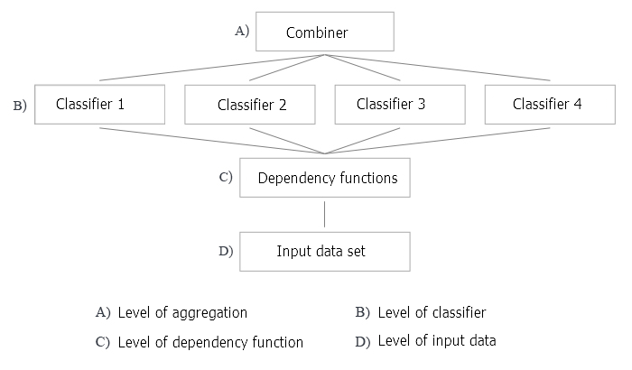
Fig.2. Four levels of creating an ensemble of classifiers
Let us discuss this in more detail.
1. Combiner
Some ensemble methods do not define a combiner. But for the methods that do, there are three types of combiners.
- Non-trainable. An example of such a method is a simple "majority voting".
- Trainable. This group includes "weighted majority voting" and "Naive Bayes", as well as the "classifier selection" approach, where the decision on a given object is made by one classifier of the ensemble.
- Meta classifier. Outputs of the base classifiers are considered as inputs for the new classifier to be trained, which becomes a combiner. This approach is called "complex generalization", "generalization through training", or simply "stacking". Building a training set for a meta classifier is one of the main problems of this combiner.
2. Building an ensemble
Should the base classifiers be trained in parallel (independently) or sequentially? An example of sequential training is AdaBoost, where the training set of each added classifier depends on the ensemble created before it.
3. Diversity
How to generate differences in the ensemble? The following options are suggested.
- Manipulate the training parameters. Use different approaches and parameters when training individual base classifiers. For example, it is possible to initialize the neuron weights in the hidden layers of each base classifier's neural network with different random variables. It is also possible to set the hyperparameters randomly.
- Manipulate the samples — take a custom bootstrap sample from the training set for each member of the ensemble.
- Manipulate the predictors — prepare a custom set of randomly determined predictors for each base classifier. This is the so-called vertical split of the training set.
4. Ensemble size
How to determine the number of classifiers in an ensemble? Is the ensemble built by simultaneous training of the required number of classifiers or iteratively by adding/removing classifiers? Possible options:
- The number is reserved in advance
- The number is set in the course of training
- Classifiers are overproduced and then selected
5. Versatility (relative to the base classifier)
Some ensemble approaches may be used with any classifier model, while others are tied to a certain type of classifier. An example of a "classifier-specific" ensemble is a Random Forest. Its base classifier is the decision tree. So, there are two variants of approaches:
- only a specific model of the base classifier can be used;
- any model of base classifier can be used.
When training and optimizing the parameters of the classifier ensemble, one should distinguish the optimization of the solution and optimization of the coverage.
- Optimization of decision making refers to the selection of a combiner for a fixed ensemble of base classifiers (level A in Figure 2).
- Optimization of alternative coverage refers to creation of diverse base classifiers with a fixed combiner (levels B, C and D in Figure 2).
This decomposition of the ensemble design reduces the complexity of the problem, so it seems reasonable.
A very detailed and deep analysis of the ensemble methods are considered in the books Combining Pattern Classifiers. Methods and Algorithms, Second Edition. Ludmila Kuncheva and Ensemble Methods. Foundations and Algorithms. They are recommended for reading.
2. Bagging
The name of the method is derived from the phrase Bootstrap AGGregatING. Bagging ensembles are created as follows:
- a bootstrap sample is extracted from the training set;
- each classifier is trained on its own sample;
- individual outputs from separate classifiers are combined into one class label. If individual outputs have the form of a class label, then a simple majority voting is used. If the output of classifiers is a continuous variable, then either averaging is applied, or the variable is converted into a class label, followed by a simple majority voting.
Let us return to Figure 2 and analyze all the levels of creating an ensemble of classifiers applied to the bagging method.
A: level of aggregation
At this level, the data obtained from the classifiers are combined and a single output is aggregated.
How do we combine individual outputs? Use a non-trainable combiner (averaging, simple majority of votes).
B: level of classifiers
At level B, all the work with classifiers takes place. Several questions arise here.
- Do we use different or the same classifiers? The same classifiers are used in the bagging approach.
- Which classifier is taken as the base classifier? We use ELM (Extreme Learning Machines).
Let us dwell on this in more detail. Selection of the classifier and its reasoning is an important part of the work. Let us list the main requirements for the base classifiers to create a high-quality ensemble.
Firstly, the classifier must be simple: deep neural networks are not recommended.
Secondly, the classifiers must be different: with different initialization, learning parameters, training sets, etc.
Thirdly, classifier speed is important: models should not take hours to train.
Fourthly, the classification models should be weak and give a prediction result slightly better than 50%.
And, finally, the instability of the classifier is important, so that the prediction results have a wide range.
There is an option that meets all these requirements. It is a special type of neural network — ELM (extreme learning machines), which were proposed as alternative learning algorithms instead of MLP. Formally, it is a fully connected neural network with one hidden layer. But without the iterative determination of weights (training) it becomes exceptionally fast. It randomly selects the weights of neurons in the hidden layer once during the initialization and then analytically determines their output weight according to the selected activation function. A detailed description of the ELM algorithm and an overview of its many varieties can be found in the attached archive.
- How many classifiers are necessary? Let us take 500 and later prune the ensemble.
- Is parallel or sequential training of classifiers used? We use parallel training, which takes place for all classifiers simultaneously.
- Which parameters of the base classifiers can be manipulated? The number of hidden layers, the activation function, the sample size of the training set. All these parameters are subject to optimization.
C: level of functions for the identified regularities
- Are all predictors used or only individual subsets for each classifier? All classifiers use one subset of predictors. But the number of predictors can be optimized.
- How to choose such a subset? In this case, special algorithms are used.
D: level of input data and their manipulations
At this level, the source data is fed to the input of the neural network for training.
How to manipulate the input data to provide a high diversity and high individual accuracy? Bootstrap samples will be used for each classifier individually. The size of the bootstrap sample is the same for all ensemble members, but it will be optimized.
To conduct experiments with ELM ensembles, there are two packages in R (elmNN, ELMR) and one package in Python (hpelm). For now, let us test the capabilities of the elmNN package, which implements the classic ELM. The elmNN package is designed for creating, training and testing using the ELM batch method. Thus, the training and test samples are ready before the training and are fed to the model once. The package is very simple.
The experiment will consist of the following stages.
- Generating the source data sets
- Arranging predictors by information importance
- Training and testing the ensemble classifiers
- Combining individual outputs of classifiers (averaging/voting)
- Ensemble pruning and its methods
- Searching for metrics of the ensemble classification quality
- Determining the optimal parameters of the ensemble members. Methods
- Training and testing the ensemble with optimal parameters
Generating the source data sets
The latest version of MRO 3.4.3 will be used for the experiments. It implements several new packages suitable for our work.
Run RStudio, go to GitHub/Part_I to download the Cotir.RData file with quotes obtained from the terminal, and fetch the FunPrepareData.R file with data preparation functions from GitHub/Part_IV.
Previously, it was determined that a set of data with imputed outliers and normalized data makes it possible to obtain better results in training with pretraining. We will use it. You can also test the other preprocessing options considered earlier.
When dividing into pretrain/train/val/test subsets, we use the first opportunity to improve the classification quality — increase the number of samples for training. The number of samples in the 'pretrain' subset will be increased to 4000.
#----Prepare-------------
library(anytime)
library(rowr)
library(elmNN)
library(rBayesianOptimization)
library(foreach)
library(magrittr)
library(clusterSim)
#source(file = "FunPrepareData.R")
#source(file = "FUN_Ensemble.R")
#---prepare----
evalq({
  dt <- PrepareData(Data, Open, High, Low, Close, Volume)
  DT <- SplitData(dt, 4000, 1000, 500, 250, start = 1)
  pre.outl <- PreOutlier(DT$pretrain)
  DTcap <- CappingData(DT, impute = T, fill = T, dither = F, pre.outl = pre.outl)
  preproc <- PreNorm(DTcap, meth = meth)
  DTcap.n <- NormData(DTcap, preproc = preproc)
}, env)
By changing the start parameter in the SplitData() function, it is possible to obtain sets shifted right by the amount of 'start'. This allows checking the quality in different parts of the price range in the future and determining how it changes in history.
Create data sets (pretrain/train/test/test1) for training and testing, gathered in the X list. Convert the objective from factor to numeric type (0.1).
#---Data X-------------
evalq({
  list(
    pretrain = list(
      x = DTcap.n$pretrain %>% dplyr::select(-c(Data, Class)) %>% as.data.frame(),
      y = DTcap.n$pretrain$Class %>% as.numeric() %>% subtract(1)
    ),
    train = list(
      x = DTcap.n$train %>% dplyr::select(-c(Data, Class)) %>% as.data.frame(),
      y = DTcap.n$train$Class %>% as.numeric() %>% subtract(1)
    ),
    test = list(
      x = DTcap.n$val %>% dplyr::select(-c(Data, Class)) %>% as.data.frame(),
      y = DTcap.n$val$Class %>% as.numeric() %>% subtract(1)
    ),
    test1 = list(
      x = DTcap.n$test %>% dplyr::select(-c(Data, Class)) %>% as.data.frame(),
      y = DTcap.n$test$Class %>% as.numeric() %>% subtract(1)
    )
  ) -> X
}, env)
Arranging predictors by information importance
Test the function clusterSim::HINoV.Mod() (see the package for more details). It ranks the variables based on clustering with different distances and methods. We will use the default parameters. You are free to experiment using other parameters. The constant numFeature <- 10 allows changing the number of the best predictors bestF fed to the model.
Calculations are performed on the X$pretrain set
require(clusterSim)
evalq({
  numFeature <- 10
  HINoV.Mod(x = X$pretrain$x %>% as.matrix(), type = "metric", s = 1, 4,
            distance =  NULL, # "d1" - Manhattan, "d2" - Euclidean,
            #"d3" - Chebychev (max), "d4" - squared Euclidean,
            #"d5" - GDM1, "d6" - Canberra, "d7" - Bray-Curtis
            method = "kmeans" ,#"kmeans" (default) , "single",
            #"ward.D", "ward.D2", "complete", "average", "mcquitty",
            #"median", "centroid", "pam"
            Index = "cRAND") -> r
  r$stopri[ ,1] %>% head(numFeature) -> bestF
}, env)
print(env$r$stopri)
      [,1]      [,2]
 [1,]    5 0.9242887
 [2,]   11 0.8775318
 [3,]    9 0.8265240
 [4,]    3 0.6093157
 [5,]    6 0.6004115
 [6,]   10 0.5730556
 [7,]    1 0.5722479
 [8,]    7 0.4730875
 [9,]    4 0.3780357
[10,]    8 0.3181561
[11,]    2 0.2960231
[12,]   12 0.1009184
The order for ranking the predictors is shown in the code listing above. The top 10 are listed below, they will be used in the future.
> colnames(env$X$pretrain$x)[env$bestF]
 [1] "v.fatl" "v.rbci" "v.ftlm" "rbci"   "v.satl" "v.stlm" "ftlm"
 [8] "v.rftl" "pcci"   "v.rstl"
Sets for the experiments are ready.
The Evaluate() function for calculating the metrics from the testing results will be taken from the previous article of this series. The value of mean(F1) will be used as the optimization (maximization) criterion. Load this function into the 'env' environment.
Creating, training and testing the ensemble
Train the ensemble of neural networks (n <- 500 units), combining them in Ens. Each neural network is trained on its own sample. The sample will be generated by extracting 7/10 examples from the training set randomly with replacement. It is necessary to set two parameters for the model: 'nh' — the number of neurons in the hidden layer and 'act' — the activation function. The package offers the following options for activation functions:
- - sig: sigmoid
- - sin: sine
- - radbas: radial basis
- - hardlim: hard-limit
- - hardlims: symmetric hard-limit
- - satlins: satlins
- - tansig: tan-sigmoid
- - tribas: triangular basis
- - poslin: positive linear
- - purelin: linear
Considering that there are 10 input variables, we first take nh = 5. The activation function is taken as actfun = "sin". The ensemble learns fast. I chose the parameters intuitively, based on my experience with neural networks. You can try other options.
#---3-----Train----------------------------
evalq({
  n <- 500
  r <- 7
  nh <- 5
  Xtrain <- X$pretrain$x[ , bestF]
  Ytrain <- X$pretrain$y
  Ens <- foreach(i = 1:n, .packages = "elmNN") %do% {
    idx <- rminer::holdout(Ytrain, ratio = r/10, mode = "random")$tr
    elmtrain(x = Xtrain[idx, ], y = Ytrain[idx],
             nhid = nh, actfun = "sin")
  }
}, env)
Let us briefly consider the calculations in the script. Define the constants n (the number of neural networks in the ensemble) and r (the size of the bootstrap sample used for training the neural network. This sample will be different for each neural network in the ensemble). nh is the number of neurons in the hidden layer. Then define the set of input data Xtrain using the main set X$pretrain and leaving only certain predictors bestF.
This produces an ensemble Ens[[500]] consisting of 500 individual neural network classifiers. Test it on the testing set Xtest obtained from the main set X$train with the best predictors bestF. The generated result is y.pr[1001, 500] - a data frame of 500 continuous predictive variables.
#---4-----predict-------------------
evalq({
  Xtest <- X$train$x[ , bestF]
  Ytest <- X$train$y
  foreach(i = 1:n, .packages = "elmNN", .combine = "cbind") %do% {
    predict(Ens[[i]], newdata = Xtest)
  } -> y.pr #[ ,n]
}, env)
Combining individual outputs of classifiers. Methods (averaging/voting)
The base classifiers of an ensemble can have the following output types:
- Class labels
- Ranked class labels, when classified with the number of classes >2
- Continuous numerical prediction/degree of support.
The base classifiers have a continuous numerical variable (the degree of support) at the output. The degrees of support for this input X can be interpreted in different ways. It can be the reliability of the proposed labels or the assessment of possible probabilities for classes. For our case, the reliability of the proposed classification labels will serve as output.
The first variant of combining is averaging: get the average value of individual outputs. Then it is converted into class labels, while the conversion threshold is taken as 0.5.
The second variant of combining is a simple majority voting. To do this, each output is first converted from a continuous variable into class labels [-1, 1] (the conversion threshold is 0.5). Then all outputs are summed, and if the result is greater than 0 then class 1 is assigned, otherwise class 0.
Using the obtained class labels, determine the metrics (Accuracy, Precision, Recall and F1).
Ensemble pruning. Methods
The number of base classifiers was initially superfluous, in order to select the best of them later. The following methods are applied for doing this:
- ordering-based pruning — selection from an ensemble ordered by a certain quality score:
- reduce-error pruning — sort the classifiers by the classification error and choose several best ones (with the least error);
- kappa pruning — order the ensemble members according to the Kappa statistic, select the required number with the least scores.
- clustering-based pruning — prediction results of the ensemble are clustered by any method, after which several representatives from each cluster are selected. Clustering methods:
- partitioning (for example SOM, k-mean);
- hierarchical;
- density-based (for example, dbscan);
- GMM-based.
- optimization-based pruning — evolutionary or genetic algorithms are used for selecting the best.
Ensemble pruning is the same selection of predictors. Therefore, the same methods can be applied to it as when selecting predictors (this has been covered in the previous articles of the series).
Selection from an ensemble ordered by classification error (reduce-error pruning) will be used for further calculations.
In total, the following methods will be used in the experiments:
- combiner method — averaging and simple majority voting;
- metrics — Accuracy, Precision, Recall and F1;
- pruning — selection from the ensemble ordered by classification error based on mean(F1).
The threshold for converting individual outputs from continuous variables into class labels is 0.5. Be forewarned: this is not the best option, but the simplest one. It can be improved later.
a) Determine the best individual classifiers of the ensemble
Determine mean(F1) of all 500 neural networks, choose several 'bestNN' with the best scores. The number of the best neural networks for majority voting must be odd, so it will be defined as: (numEns*2 + 1).
#---5-----best----------------------
evalq({
  numEns <- 3
  foreach(i = 1:n, .combine = "c") %do% {
    ifelse(y.pr[ ,i] > 0.5, 1, 0) -> Ypred
    Evaluate(actual = Ytest, predicted = Ypred)$Metrics$F1 %>%
      mean()
  } -> Score
  Score %>% order(decreasing = TRUE) %>% head((numEns*2 + 1)) -> bestNN
  Score[bestNN] %>% round(3)
}, env)
[1] 0.720 0.718 0.718 0.715 0.713 0.713 0.712
Let us briefly consider the calculations in the script. In the foreach() loop, convert the continuous prediction y.pr[ ,i] of each neural network into numerical [0,1], determine mean(F1) of this prediction and output the value as the vector Score[500]. Then sort the data of the vector Score in descending order, determine the indexes of bestNN neural networks with the best (highest) scores. Output the metrics values of these best members of the Score[bestNN], rounded to 3 decimal places. As you can see, the individual results are not very high.
Note: each training and testing run will produce a different result, as the samples and the starting initialization of the neural networks will be different!
So, the best individual classifiers in the ensemble have been identified. Let us test them on samples X$test and X$test1, using the following combination methods: averaging and simple majority voting.
b) Averaging
#---6----test averaging(test)--------
evalq({
  n <- len(Ens)
  Xtest <- X$test$x[ , bestF]
  Ytest <- X$test$y
  foreach(i = 1:n, .packages = "elmNN", .combine = "+") %:%
    when(i %in% bestNN) %do% {
    predict(Ens[[i]], newdata = Xtest)} %>%
    divide_by(length(bestNN)) -> ensPred
  ifelse(ensPred > 0.5, 1, 0) -> ensPred
  Evaluate(actual = Ytest, predicted = ensPred)$Metrics[ ,2:5] %>%
    round(3)
}, env)
Accuracy Precision Recall    F1
0     0.75     0.723  0.739 0.731
1     0.75     0.774  0.760 0.767
A few words about the calculations in the script. Determine the size of the ensemble n, inputs Xtest and objective Ytest, using the main set X$test. Then, in the foreach loop (only when the index is equal to the 'bestNN' indexes), calculate the predictions of these best neural networks, sum them, divide by the number of the best neural networks. Convert the output from a continuous variable into a numerical variable (0,1) and calculate the metrics. As you can see, the classification quality scores are much higher than those of individual classifiers.
Perform the same test on the X$test1 set, located next to X$test. Estimate the quality.
#--6.1 ---test averaging(test1)---------
evalq({
  n <- len(Ens)
  Xtest <- X$test1$x[ , bestF]
  Ytest <- X$test1$y
  foreach(i = 1:n, .packages = "elmNN", .combine = "+") %:%
    when(i %in% bestNN) %do% {
      predict(Ens[[i]], newdata = Xtest)} %>%
    divide_by(length(bestNN)) -> ensPred
  ifelse(ensPred > 0.5, 1, 0) -> ensPred
  Evaluate(actual = Ytest, predicted = ensPred)$Metrics[ ,2:5] %>%
    round(3)
}, env)
Accuracy Precision Recall    F1
0    0.745     0.716  0.735 0.725
1    0.745     0.770  0.753 0.761
The quality of the classification has remained practically unchanged and remains quite high. This result shows that the ensemble of neural network classifiers retains a high quality of classification after training and pruning for a much longer period (in our example, 750 bars) than the DNN obtained in the previous article.
c) Simple majority voting
Let us determine the metrics of the prediction obtained from the best classifiers of the ensemble, but combined by simple voting. First, convert the continuous predictions of the best classifiers into class labels (-1/+1), then sum all the prediction labels. If the sum is greater than 0, then class 1 is output, otherwise — class 0. First, test everything on the X$test set:
#--7 --test--voting(test)--------------------
evalq({
  n <- len(Ens)
  Xtest <- X$test$x[ , bestF]
  Ytest <- X$test$y
  foreach(i = 1:n, .packages = "elmNN", .combine = "cbind") %:%
    when(i %in% bestNN) %do% {
    predict(Ens[[i]], newdata = Xtest)
  } %>%
    apply(2, function(x) ifelse(x > 0.5, 1, -1)) %>%
    apply(1, function(x) sum(x)) -> vot
  ifelse(vot > 0, 1, 0) -> ClVot
  Evaluate(actual = Ytest, predicted = ClVot)$Metrics[ ,2:5] %>%
    round(3)
}, env)
Accuracy Precision Recall    F1
0    0.745     0.716  0.735 0.725
1    0.745     0.770  0.753 0.761
The result is practically the same as the result for averaging. Test on the X$test1 set:
#--7.1 --test--voting(test1)--------------------
evalq({
  n <- len(Ens)
  Xtest <- X$test1$x[ , bestF]
  Ytest <- X$test1$y
  foreach(i = 1:n, .packages = "elmNN", .combine = "cbind") %:%
    when(i %in% bestNN) %do% {
      predict(Ens[[i]], newdata = Xtest)
    } %>%
    apply(2, function(x) ifelse(x > 0.5, 1, -1)) %>%
    apply(1, function(x) sum(x)) -> vot
  ifelse(vot > 0, 1, 0) -> ClVot
  Evaluate(actual = Ytest, predicted = ClVot)$Metrics[ ,2:5] %>%
    round(3)
}, env)
Accuracy Precision Recall    F1
0    0.761     0.787  0.775 0.781
1    0.761     0.730  0.743 0.737
Unexpectedly, the result turned out to be better than all previous ones, and this is despite the fact that the X$test1 set is located after X$test.
This means that the classification quality of the same ensemble on the same data but with different combination method can vary greatly.
Despite the fact that the hyperparameters of the individual classifiers in the ensemble were chosen intuitively and obviously are not optimal, a high and stable quality of classification was obtained, both using averaging and a simple majority voting.
Summarize all the above. Schematically, the whole process of creating and testing an ensemble of neural networks can be divided into 4 stages:
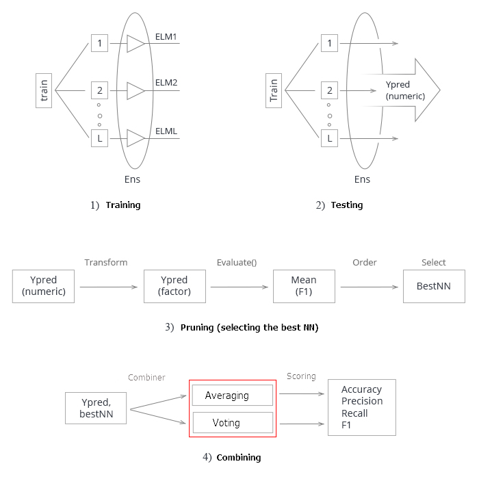
Fig.3. Structure of training and testing the ensemble of neural networks with the averaging/voting combiner
1. Training the ensemble. Train L neural networks on random samples (bootstrap) from the training set. Obtain the ensemble of trained neural networks.
2. Test the ensemble of neural networks on the testing set. Obtain continuous predictions of individual classifiers.
3. Prune the ensemble, choosing the best n by a certain the classification quality criterion. In this case, it is mean(F1).
4. Using continuous predictions of the best individual classifiers, combine them with the help of either averaging or simple majority voting. After that, determine the metrics.
The two last steps (pruning and combination) have multiple implementation options. At the same time, successful pruning of the ensemble (correct identification of the best) can significantly increase the performance. In this case, it is finding the optimal conversion threshold of a continuous prediction into a numerical one. Therefore, finding the optimal parameters at these stages is a laborious task. These stages are best performed automatically and with the best result. Do we have the ability to do this and to improve the ensemble's quality scores? There are at least two ways to do this, we will check them.
- Optimize the hyperparameters of individual classifiers of the ensemble (Bayesian optimizer).
- DNN will be used as a combiner of the ensemble's individual outputs. Generalization will be performed through learning.
Determine the optimal parameters of the ensemble's individual classifiers. Methods
Individual classifiers in our ensemble are ELM neural networks. The main feature of ELM is that their properties and quality mainly depend on random initialization of the hidden layer's neuron weights. Other things being equal (the number of neurons and activation functions), each training run will produce a new neural network.
This feature of ELM is just perfect for creating ensembles. In the ensemble, not only do we initialize the weights of each classifier with random values, but also provide each classifier with a separate randomly generated training sample.
But in order to select the best hyperparameters of a neural network, its quality has to depend only on the changes of a given hyperparameter and nothing else. Otherwise, the meaning of the search is lost.
A contradiction arises: on the one hand, we need an ensemble with as diverse members as possible, and on the other hand, an ensemble with diverse but permanent members.
A reproducible permanent variety is required.
Is it possible? Let us use an example of ensemble training to show this. The "doRNG" (Reproducible random number generation RNG) package will be used. For reproducibility of results, it is better to perform calculations in one thread.
Begin a new experiment with a clean global environment. Load the quotes and the necessary libraries again, define and sort the source data once more and re-select numFeature best predictors. Run it all in one script.
#----Prepare-------------
library(anytime)
library(rowr)
library(elmNN)
library(rBayesianOptimization)
library(foreach)
library(magrittr)
library(clusterSim)
library(doRNG)
#source(file = "FunPrepareData.R")
#source(file = "FUN_Ensemble.R")
#---prepare----
evalq({
  dt <- PrepareData(Data, Open, High, Low, Close, Volume)
  DT <- SplitData(dt, 4000, 1000, 500, 250, start = 1)
  pre.outl <- PreOutlier(DT$pretrain)
  DTcap <- CappingData(DT, impute = T, fill = T, dither = F, pre.outl = pre.outl)
  preproc <- PreNorm(DTcap, meth = meth)
  DTcap.n <- NormData(DTcap, preproc = preproc)
#--1-Data X-------------
  list(
    pretrain = list(
      x = DTcap.n$pretrain %>% dplyr::select(-c(Data, Class)) %>% as.data.frame(),
      y = DTcap.n$pretrain$Class %>% as.numeric() %>% subtract(1)
    ),
    train = list(
      x = DTcap.n$train %>% dplyr::select(-c(Data, Class)) %>% as.data.frame(),
      y = DTcap.n$train$Class %>% as.numeric() %>% subtract(1)
    ),
    test = list(
      x = DTcap.n$val %>% dplyr::select(-c(Data, Class)) %>% as.data.frame(),
      y = DTcap.n$val$Class %>% as.numeric() %>% subtract(1)
    ),
    test1 = list(
      x = DTcap.n$test %>% dplyr::select(-c(Data, Class)) %>% as.data.frame(),
      y = DTcap.n$test$Class %>% as.numeric() %>% subtract(1)
    )
  ) -> X
#---2--bestF-----------------------------------
#require(clusterSim)
  numFeature <- 10
  HINoV.Mod(x = X$pretrain$x %>% as.matrix(), type = "metric", s = 1, 4,
            distance =  NULL, # "d1" - Manhattan, "d2" - Euclidean,
            #"d3" - Chebychev (max), "d4" - squared Euclidean,
            #"d5" - GDM1, "d6" - Canberra, "d7" - Bray-Curtis
            method = "kmeans" ,#"kmeans" (default) , "single",
            #"ward.D", "ward.D2", "complete", "average", "mcquitty",
            #"median", "centroid", "pam"
            Index = "cRAND") %$% stopri[ ,1] -> orderX
  orderX %>% head(numFeature) -> bestF
}, env)
All the necessary initial data are ready. Train the ensemble of neural networks:
#---3-----Train----------------------------
evalq({
  Xtrain <- X$pretrain$x[ , bestF]
  Ytrain <- X$pretrain$y
  setMKLthreads(1)
  n <- 500
  r <- 7
  nh <- 5
  k <- 1
  rng <- RNGseq(n, 12345)
  Ens <- foreach(i = 1:n, .packages = "elmNN") %do% {
    rngtools::setRNG(rng[[k]])
    k <- k + 1
    idx <- rminer::holdout(Ytrain, ratio = r/10, mode = "random")$tr
    elmtrain(x = Xtrain[idx, ], y = Ytrain[idx],
             nhid = nh, actfun = "sin")
  }
  setMKLthreads(2)
}, env)
What happens during the execution? Define the input and output data for training (Xtrain, Ytrain), set the MKL library to single-threaded mode. Initialize certain constants by creating a sequence of random numbers rng, which will initialize the random number generator at each new iteration of foreach().
After completing the iterations, do not forget to set MKL back to multithreaded mode. In single-threaded mode, the calculation results are slightly worse.
Thus, we obtain an ensemble with different individual classifiers, but at each rerun of the training, these classifiers of the ensemble will remain unchanged. This can easily be verified by repeating the calculations of 4 stages (train/predict/best/test) several times. Calculation order: train/predict/best/test_averaging/test_voting.
#---4-----predict-------------------
evalq({
  Xtest <- X$train$x[ , bestF]
  Ytest <- X$train$y
  foreach(i = 1:n, .packages = "elmNN", .combine = "cbind") %do% {
    predict(Ens[[i]], newdata = Xtest)
  } -> y.pr #[ ,n]
}, env)
#---5-----best----------------------
evalq({
  numEns <- 3
  foreach(i = 1:n, .combine = "c") %do% {
    ifelse(y.pr[ ,i] > 0.5, 1, 0) -> Ypred
    Evaluate(actual = Ytest, predicted = Ypred)$Metrics$F1 %>%
      mean()
  } -> Score
  Score %>% order(decreasing = TRUE) %>% head((numEns*2 + 1)) -> bestNN
  Score[bestNN] %>% round(3)
}, env)
# [1] 0.723 0.722 0.722 0.719 0.716 0.714 0.713
#---6----test averaging(test)--------
evalq({
  n <- len(Ens)
  Xtest <- X$test$x[ , bestF]
  Ytest <- X$test$y
  foreach(i = 1:n, .packages = "elmNN", .combine = "+") %:%
    when(i %in% bestNN) %do% {
      predict(Ens[[i]], newdata = Xtest)} %>%
    divide_by(length(bestNN)) -> ensPred
  ifelse(ensPred > 0.5, 1, 0) -> ensPred
  Evaluate(actual = Ytest, predicted = ensPred)$Metrics[ ,2:5] %>%
    round(3)
}, env)
# Accuracy Precision Recall F1
# 0 0.75 0.711 0.770 0.739
# 1 0.75 0.790 0.734 0.761
#--7 --test--voting(test)--------------------
evalq({
  n <- len(Ens)
  Xtest <- X$test$x[ , bestF]
  Ytest <- X$test$y
  foreach(i = 1:n, .packages = "elmNN", .combine = "cbind") %:%
    when(i %in% bestNN) %do% {
      predict(Ens[[i]], newdata = Xtest)
    } %>%
    apply(2, function(x) ifelse(x > 0.5, 1, -1)) %>%
    apply(1, function(x) sum(x)) -> vot
  ifelse(vot > 0, 1, 0) -> ClVot
  Evaluate(actual = Ytest, predicted = ClVot)$Metrics[ ,2:5] %>%
    round(3)
}, env)
# Accuracy Precision Recall F1
# 0 0.749 0.711 0.761 0.735
# 1 0.749 0.784 0.738 0.760
No matter how many times these calculations are repeated (naturally, with the same parameters), the result will remain unchanged. This is exactly what we need to optimize the hyperparameters of the neural networks comprising the ensemble.
First, define the list of hyperparameters to be optimized, find their value ranges, and write a fitness function to return the optimization (maximization) criterion and the prediction of the ensemble. The quality of individual classifiers is affected by four parameters:
- the number of predictors in the input data;
- size of the sample used for training;
- the number of neurons in the hidden layer;
- activation function.
Let us list the hyperparameters and their value ranges:
evalq({
  #type of activation function.
  Fact <- c("sig", #: sigmoid
            "sin", #: sine
            "radbas", #: radial basis
            "hardlim", #: hard-limit
            "hardlims", #: symmetric hard-limit
            "satlins", #: satlins
            "tansig", #: tan-sigmoid
            "tribas", #: triangular basis
            "poslin", #: positive linear
            "purelin") #: linear
  bonds <- list(
    numFeature = c(3L, 12L),
    r = c(1L, 10L),
    nh <- c(1L, 50L),
    fact = c(1L, 10L)
  )
}, env)
Let us examine the code above in more detail. There, Fact is a vector of possible activation functions. The list bonds defines the parameters to be optimized and their value ranges.
- numFeature — the number of predictors fed as input; minimum 3, maximum 12;
- r — proportion of the training set used in bootstrap. Before calculating, divide it by 10.
- nh — the number of neurons in the hidden layer; minimum 1, maximum 50.
- fact — index of the activation function in the Fact vector.
Determine the fitness function.
#---Fitnes -FUN-----------
evalq({
  Ytrain <- X$pretrain$y
  Ytest <- X$train$y
  Ytest1 <- X$test$y
  n <- 500
  numEns <- 3
fitnes <- function(numFeature, r, nh, fact){
    bestF <- orderX %>% head(numFeature)
    Xtrain <- X$pretrain$x[ , bestF]
    setMKLthreads(1)
    k <- 1
    rng <- RNGseq(n, 12345)
    #---train---
    Ens <- foreach(i = 1:n, .packages = "elmNN") %do% {
      rngtools::setRNG(rng[[k]])
      idx <- rminer::holdout(Ytrain, ratio = r/10, mode = "random")$tr
      k <- k + 1
      elmtrain(x = Xtrain[idx, ], y = Ytrain[idx],
               nhid = nh, actfun = Fact[fact])
    }
    setMKLthreads(2)
    #---predict---
    Xtest <- X$train$x[ , bestF]
    foreach(i = 1:n, .packages = "elmNN", .combine = "cbind") %do% {
      predict(Ens[[i]], newdata = Xtest)
    } -> y.pr #[ ,n]
   #---best---
    foreach(i = 1:n, .combine = "c") %do% {
      ifelse(y.pr[ ,i] > 0.5, 1, 0) -> Ypred
      Evaluate(actual = Ytest, predicted = Ypred)$Metrics$F1 %>%
        mean()
    } -> Score
    Score %>% order(decreasing = TRUE) %>%
      head((numEns*2 + 1)) -> bestNN
    #---test-aver--------
    Xtest1 <- X$test$x[ , bestF]
    foreach(i = 1:n, .packages = "elmNN", .combine = "+") %:%
      when(i %in% bestNN) %do% {
        predict(Ens[[i]], newdata = Xtest1)} %>%
      divide_by(length(bestNN)) -> ensPred
    ifelse(ensPred > 0.5, 1, 0) -> ensPred
    Evaluate(actual = Ytest1, predicted = ensPred)$Metrics$F1 %>%
      mean() %>% round(3) -> Score
    return(list(Score = Score, Pred = ensPred))
   }
}, env)
Here are some details about the script. Move the calculation of the objectives (Ytrain, Ytest, Ytest1) out of the fitness function, as they are not changed during the parameter search. Initialize the constants:
n — the number of neural networks in the ensemble;
numEns — the number of the best individual classifiers (numEns*2 + 1), the predictions of which are to be combined.
The fitnes() function has 4 formal parameters, which should be optimized. Later in the function, train the ensemble, calculate predict and determine bestNN of the best ones, step by step. In the end, combine the predictions of these best using averaging and calculate the metrics. The function returns a list, containing the optimization criterion Score = mean(F1) and the prediction. We will optimize the ensemble that uses combination by averaging. Fitness function for optimizing the hyperparameters of the ensemble with a simple majority voting is similar, except for the final part. You can perform the optimization yourself.
Let us check the fitness function operability and its execution time:
#----------
evalq(
  system.time(
   res <- fitnes(numFeature = 10, r = 7, nh = 5, fact = 2)
  )
, env)
 user  system elapsed
   8.65    0.19    7.86
It took about 9 seconds to get the result for all calculations.
> env$res$Score
[1] 0.761
Now we can start optimization of the hyperparameters with 10 random initialization points and 20 iterations. We are looking for the best result.
#------
evalq(
  OPT_Res <- BayesianOptimization(fitnes, bounds = bonds,
                                   init_grid_dt = NULL, init_points = 10,
                                   n_iter = 20, acq = "ucb", kappa = 2.576,
                                   eps = 0.0, verbose = TRUE)
, envir = env)
Best Parameters Found:
  Round = 23  numFeature = 8.0000  r = 3.0000 nh = 3.0000  fact = 7.0000        Value = 0.7770
Order the optimization history by Value and select 10 best scores:
evalq({
  OPT_Res %$% History %>% dplyr::arrange(desc(Value)) %>% head(10) %>%
    dplyr::select(-Round) -> best.init
  best.init
}, env)
 numFeature r nh fact Value
1           8 3  3    7 0.777
2           8 1  5    7 0.767
3           8 3  2    7 0.760
4          10 7  9    8 0.759
5           8 5  4    7 0.758
6           8 2  7    8 0.756
7           8 6  9    7 0.755
8           8 3  4    8 0.754
9           9 2 13    9 0.752
10         11 2 24    4 0.751
Interpret the obtained hyperparameters of the best result. The number of predictors is 8, sample size is 0.3, the number of neurons in the hidden layer is 3, activation function is "radbas". This once again proves that the Bayesian optimization gives a wide spectrum of various models, which are unlikely to be derived intuitively. It is necessary to repeat the optimization several times and select the best result.
So, the optimal hyperparameters of training have been found. Test the ensemble with them.
Training and testing the ensemble with optimal parameters
Test the ensemble, trained with the optimal parameters obtained above, on the testing set. Determine the best members of the ensemble, combine their results by averaging and see the final metrics. The script is shown below.
When training the ensemble of neural networks, create it in the same way as during optimization.
#--1-Train--optEns-predict--best--test-average------------------------
evalq({
  Ytrain <- X$pretrain$y
  Ytest <- X$train$y
  Ytest1 <- X$test$y
  n <- 500
  numEns <- 3
  #--BestParams--------------------------
  best.par <- OPT_Res$Best_Par %>% unname
  numFeature <- best.par[1] # 8L
  r <- best.par[2]          # 3L
  nh <- best.par[3]         # 3L
  fact <- best.par[4]       # 7L
  bestF <- orderX %>% head(numFeature)
  Xtrain <- X$pretrain$x[ , bestF]
  setMKLthreads(1)
  k <- 1
  rng <- RNGseq(n, 12345)
  #---train---
  OptEns <- foreach(i = 1:n, .packages = "elmNN") %do% {
    rngtools::setRNG(rng[[k]])
    idx <- rminer::holdout(Ytrain, ratio = r/10, mode = "random")$tr
    k <- k + 1
    elmtrain(x = Xtrain[idx, ], y = Ytrain[idx],
             nhid = nh, actfun = Fact[fact])
  }
  setMKLthreads(2)
  #---predict---
  Xtest <- X$train$x[ , bestF]
  foreach(i = 1:n, .packages = "elmNN", .combine = "cbind") %do% {
    predict(OptEns[[i]], newdata = Xtest)
  } -> y.pr #[ ,n]
  #---best---
  foreach(i = 1:n, .combine = "c") %do% {
    ifelse(y.pr[ ,i] > 0.5, 1, 0) -> Ypred
    Evaluate(actual = Ytest, predicted = Ypred)$Metrics$F1 %>%
      mean()
  } -> Score
  Score %>% order(decreasing = TRUE) %>%
    head((numEns*2 + 1)) -> bestNN
  #---test-aver--------
  Xtest1 <- X$test$x[ , bestF]
  foreach(i = 1:n, .packages = "elmNN", .combine = "+") %:%
    when(i %in% bestNN) %do% {
      predict(OptEns[[i]], newdata = Xtest1)} %>%
    divide_by(length(bestNN)) -> ensPred
  ifelse(ensPred > 0.5, 1, 0) -> ensPred
  Evaluate(actual = Ytest1, predicted = ensPred)$Metrics[ ,2:5] %>%
    round(3) -> OptScore
  caret::confusionMatrix(Ytest1, ensPred) -> cm
}, env)
Let us see the results of 7 best neural networks of the ensemble:
> env$Score[env$bestNN]
[1] 0.7262701 0.7220685 0.7144137 0.7129644 0.7126606 0.7101981  0.7099502
The result after averaging the best neural networks:
> env$OptScore
  Accuracy Precision Recall    F1
0    0.778     0.751  0.774 0.762
1    0.778     0.803  0.782 0.793
> env$cm
Confusion Matrix and Statistics

          Reference
Prediction   0   1
         0 178  52
         1  59 212

               Accuracy : 0.7784
                 95% CI : (0.7395, 0.8141)
    No Information Rate : 0.5269
    P-Value [Acc > NIR] : <2e-16

                  Kappa : 0.5549
 Mcnemar's Test P-Value : 0.569

            Sensitivity : 0.7511
            Specificity : 0.8030
         Pos Pred Value : 0.7739
         Neg Pred Value : 0.7823
             Prevalence : 0.4731
         Detection Rate : 0.3553
   Detection Prevalence : 0.4591
      Balanced Accuracy : 0.7770

       'Positive' Class : 0
This result is noticeably better than that of any individual neural network in the ensemble and is comparable to the results of DNN with the optimal parameters obtained in the previous article in this series.
Conclusion
- Ensembles of neural network classifiers, composed of simple and fast ELM neural networks, show a classification quality comparable to that of more complex models (DNN).
- Optimization of hyperparameters of individual classifiers in the ensemble gives an increase in the classification quality of up to Acc = 0.77(95% CI = 0.73 - 0.81).
- Classification quality of an ensemble with averaging and an ensemble with majority voting are approximately the same.
- After training, the ensemble retains its classification quality to a depth of more than half the size of the training set. In this case, the quality is retained for up to 750 bars, which is significantly higher than the same figure obtained on DNN (250 bars).
- It is possible to significantly increase the classification quality of the ensemble by optimizing the conversion threshold of the continuous predictive variable into a numerical one (calibration, optimal CutOff, genetic search).
- The classification quality of the ensemble can also be increased by using a trainable model (stacking) as a combiner. It can be a neural network or an ensemble of neural networks. In the next part of the article, these two variants of stacking will be tested. We will test new features provided by the TensorFlow group of libraries for constructing a neural network.
Attachments
GitHub/PartVI contains:
- FUN_Ensemble.R — functions required for performing all calculations described in this article.
- RUN_Ensemble.R — scripts for creating, training and testing the ensemble.
- Optim_Ensemble.R — scripts for optimizing the hyperparameters of the neural networks in the ensemble.
- SessionInfo_RunEns.txt — packages used to create and test the ensemble.
- SessionInfo_OptEns.txt — packages used to optimize the hyperparameters of the NN ensemble.
- ELM.zip — archive of articles on ELM neural networks.
Translated from Russian by MetaQuotes Ltd.
Original article: https://www.mql5.com/ru/articles/4227
Warning: All rights to these materials are reserved by MetaQuotes Ltd. Copying or reprinting of these materials in whole or in part is prohibited.
This article was written by a user of the site and reflects their personal views. MetaQuotes Ltd is not responsible for the accuracy of the information presented, nor for any consequences resulting from the use of the solutions, strategies or recommendations described.

 Applying the Monte Carlo method for optimizing trading strategies
 Comparative analysis of 10 flat trading strategies
 How to analyze the trades of the Signal selected in the chart
- Free trading apps
- Over 8,000 signals for copying
- Economic news for exploring financial markets
You agree to website policy and terms of use
Tried an ensemble of 10 DNN Darch pieces, averaging the forecasts of the top 10. On data similar to yours, but from my DC.
No improvement, the average prediction (osh=33%) is just below the best (osh=31%). The worst was with error=34%.
DNNs are trained well - for 100 epochs.
Apparently ensembles work well on a large number of undertrained or weak networks like Elm.
Of course, it is better to use weak and unstable models in ensembles. But you can also create ensembles with strict ones, but the technique is a bit different. If the size allows, I will show in the next article how to create an ensemble using TensorFlow. In general, the topic of ensembles is very large and interesting. For example, you can build a RandomForest with ELM neural networks or any other weak models as nodes (see gensemble package).
Success
Обсуждение и вопросы по коду можно сделать в ветке
Удачи
Discussion and questions on the code can be done in the branch
Good luck