MetaTrader 5 Machine Learning Blueprint (Part 20): Denoising, Detoning, and Clustering the Feature Correlation Matrix

Table of Contents

1. Introduction
2. Why Cluster Feature Importance Needs a Clean Correlation Matrix
3. The Marcenko–Pastur Theorem
4. Fitting the Noise Ceiling: Raw Bar Count vs. Effective Sample Size
5. Denoising the Correlation Matrix
6. Detoning: Removing the Market Component
7. A Representative Feature Panel
8. Cluster Recovery, Before and After
9. Practical Considerations
10. Conclusion
11. Attached Files

Introduction

Part 9 closed with an explicit prerequisite: the pipeline described there assumes the feature set has already been validated and curated, and it named clustered importance directly as one of the techniques still owed to the reader. This article is the first half of that promise. It does not compute feature importance yet. It builds the object that clustered MDI and MDA in the next article depend on: a correlation matrix that has been cleaned of estimation noise and the shared market-mode component, both of which distort clustering.

This matters specifically for meta-labeling. Every meta-labeling model in this series takes a side prediction from a primary model and asks a secondary classifier whether to act on it, using whatever feature panel is on hand at the time. That panel has grown across the Feature Engineering for ML series. It now includes fractional differentiation levels, time-of-day encodings, microstructure estimators, entropy measures, fractal features, and trend-scanning statistics, all computed from the same underlying price path. Features built from a shared price series are not independent by construction, and several of them are deliberately redundant (multiple lookback windows of the same estimator).

Feeding that panel directly into MDI or MDA produces the substitution effect described in AFML Chapter 8. Correlated features split credit for the same signal and rank below their true contribution. Machine Learning for Asset Managers (MLAM) Section 6.5 addresses this with clustered importance, computed on groups of similar features rather than on individual columns. Clustering, in turn, only works reliably on a correlation matrix that has been denoised and detoned first; MLAM's own worked example says so explicitly, skipping that step only to stress-test the clustering algorithm's robustness, not as a recommendation for practice.

The chain is therefore: denoise and detone the feature correlation matrix (MLAM Chapter 2), cluster it with the optimal number of clusters (ONC) algorithm (MLAM Chapter 4), then compute clustered MDI and MDA on the result (MLAM Section 6.5, next article). This article covers the first two links. It also revisits a question neither AFML nor MLAM addresses directly: what sample size should the Marcenko–Pastur fit actually use when the underlying bars are serially correlated, as H1 FX bars are.

Why Cluster Feature Importance Needs a Clean Correlation Matrix

A sample correlation matrix estimated from a finite window is never the true correlation matrix. Two distinct sources of contamination sit inside it, and clustering is sensitive to both.

The first is estimation noise. With N features and T observations, a matrix built from purely random, uncorrelated data still produces a spread of nonzero sample correlations and a spread of sample eigenvalues away from 1, purely from finite-sample variation. Random matrix theory gives the exact shape of that spread under the null of no correlation; anything inside it is indistinguishable from noise, and anything outside it is evidence of real structure. Section 7 below fits that shape to the feature panel used in this article.

The second is a shared market-mode component. Features derived from the same instrument's price path tend to share exposure to the prevailing regime: a trending, high-volatility stretch inflates trend, volatility, and several microstructure estimators simultaneously, independent of whatever family-specific signal each feature is meant to isolate. That shared component shows up as an unusually large first eigenvalue with roughly uniform loadings across the affected features. MLAM Section 2.6 makes the mechanical consequence explicit: clustering struggles to separate feature families when the correlation matrix carries a strong common tone, because every feature looks somewhat similar to every other feature through that shared channel.

Denoising addresses the first problem. Detoning addresses the second. Both are prerequisites for clustering that this article treats as a single pipeline, applied before any importance computation runs.

The Marcenko–Pastur Theorem

The Marcenko–Pastur (MP) theorem describes the limiting distribution of eigenvalues of a correlation matrix estimated from N independent, identically distributed random variables observed over T periods as N and T both grow with a fixed ratio. Writing q = T/N and σ² for the variance explained by pure noise, the eigenvalues under this null concentrate between

λmin = σ²(1 − √(1/q))²  and  λmax = σ²(1 + √(1/q))²

with a known closed-form density between those two bounds. Two things about this ratio matter for what follows. First, q is defined as observations per variable, T/N, not the other way around: a large q (lots of data relative to the number of features) narrows the noise band toward σ², and a small q widens it. Getting this backward silently inflates the noise band by orders of magnitude for typical panels, since 1/q then becomes T/N instead of N/T. Second, σ² is not assumed; it is fit to the data by minimizing the squared distance between this theoretical density and a kernel density estimate of the panel's own empirical eigenvalue histogram.

Any eigenvalue above the fitted λmax is more extreme than pure noise can produce and is treated as signal. Everything at or below it is statistically indistinguishable from noise, regardless of how visually large or small the number looks.

Fitting the Noise Ceiling: Raw Bar Count vs. Effective Sample Size

The fitting routine itself is direct: evaluate the theoretical MP density at a trial σ², compare it against a kernel density estimate of the observed eigenvalues over the same support, and minimize the squared error over σ². This mirrors MLAM Snippet 2.2, with one implementation detail worth flagging explicitly because it is easy to get quietly wrong: the kernel bandwidth here must be an absolute value in eigenvalue units (sklearn.neighbors.KernelDensity(bandwidth=...)), not a relative scale factor (scipy.stats.gaussian_kde's bw_method, which rescales by the data's own standard deviation). Passing the same numeric bandwidth to the wrong implementation does not raise an error; it just returns a badly biased fit that collapses to the search boundary.

def mp_pdf(var, q, pts=1000):
    e_min = var * (1 - (1.0 / q) ** 0.5) ** 2
    e_max = var * (1 + (1.0 / q) ** 0.5) ** 2
    e_val = np.linspace(e_min, e_max, pts)
    pdf = q / (2 * np.pi * var * e_val) * ((e_max - e_val) * (e_val - e_min)) ** 0.5
    return pd.Series(pdf, index=e_val)


def fit_kde(obs, b_width=0.15, x=None):
    """Absolute-bandwidth KDE of the empirical eigenvalue distribution."""
    obs = np.asarray(obs).reshape(-1, 1)
    kde = KernelDensity(kernel="gaussian", bandwidth=b_width).fit(obs)
    x = np.unique(obs).reshape(-1, 1) if x is None else np.asarray(x).reshape(-1, 1)
    return pd.Series(np.exp(kde.score_samples(x)), index=x.flatten())


def err_pdfs(var, e_val, q, b_width, pts=1000):
    pdf0 = mp_pdf(var[0], q, pts)
    pdf1 = fit_kde(e_val, b_width, x=pdf0.index.values)
    return float(np.sum((pdf1 - pdf0) ** 2))


def find_max_eval(e_val, q, b_width=0.15):
    out = minimize(lambda v: err_pdfs(v, e_val, q, b_width),
                    x0=np.array([0.5]), bounds=((1e-5, 1 - 1e-5),))
    var = out["x"][0] if out["success"] else 1.0
    e_max = var * (1 + (1.0 / q) ** 0.5) ** 2
    return e_max, var

Both convention mistakes above (the q inversion and the bandwidth type) are silent. find_max_eval still returns a number; it is simply the wrong number, and the reported factor count will look plausible without being defensible. Either one is worth a dedicated unit test against a synthetic, known-answer covariance matrix before trusting the fit on a real feature panel.

A separate question, and the one that actually motivated this section, is what value of T to use in the first place. The theorem assumes independent observations. H1 FX bars are not independent; adjacent bars share regime, volatility clustering, and microstructural persistence, so T = raw bar count overstates the amount of independent information the panel actually contains. This is the same effective-sample-size correction already applied elsewhere in this series to sequential bootstrap and concurrent-label weighting, and it belongs here too: an AR(1)-style adjustment based on the panel's own average lag-1 autocorrelation gives a more defensible Teff.

def effective_sample_size(X, t_raw):
    """Average lag-1 autocorrelation across columns -> AR(1) effective T."""
    rhos = [np.corrcoef(X[:-1, j], X[1:, j])[0, 1] for j in range(X.shape[1])]
    rho_bar = float(np.mean(rhos))
    t_eff = t_raw * (1 - rho_bar) / (1 + rho_bar)
    return t_eff, rho_bar

Neither AFML nor MLAM addresses this adjustment directly; both treat T as given. Treating raw bar count as T without checking the panel's own autocorrelation is an unstated independence assumption, not a neutral default, and below shows the numeric consequence on the actual feature panel used in this article.

Denoising the Correlation Matrix

Once the noise ceiling λmax and the corresponding factor count nfacts are known, MLAM Section 2.5 gives two ways to clean the matrix. The constant residual eigenvalue method keeps the top nfacts eigenvalues and eigenvectors untouched and collapses every eigenvalue below the ceiling to their shared average, preserving the trace of the matrix while flattening everything classified as noise:

def cov2corr(cov):
    std = np.sqrt(np.diag(cov))
    corr = cov / np.outer(std, std)
    corr[corr < -1], corr[corr > 1] = -1, 1
    return corr


def denoised_corr(e_val, e_vec, n_facts, labels=None):
    """Constant residual eigenvalue method (MLAM eq. 2.5)."""
    e_val_ = e_val.copy()   # get_pca already returns a 1D vector
    if n_facts < e_val_.shape[0]:
        e_val_[n_facts:] = e_val_[n_facts:].sum() / (e_val_.shape[0] - n_facts)
    corr1 = cov2corr(e_vec @ np.diag(e_val_) @ e_vec.T)
    return pd.DataFrame(corr1, index=labels, columns=labels) if labels is not None else corr1

Targeted shrinkage is the alternative. Instead of fixing noise eigenvalues to a constant, it applies a shrinkage weight α to the noise eigenvectors' contribution while leaving signal eigenvectors untouched (α → 0 implies total shrinkage). MLAM's own Monte Carlo comparison in Section 2.7 finds the constant residual eigenvalue method the more effective of the two for a minimum-variance portfolio benchmark, with targeted shrinkage adding little on top of it; that result is why the constant residual eigenvalue method is the one used for the rest of this article. Both are already available as tested methods on the RiskEstimators-equivalent used elsewhere in this pipeline (unit-tested to four decimal places against MLAM's own reference values), so production code should call that shared implementation rather than duplicate the routine above; the version here is the minimal, self-contained form for readers following along independently.

Detoning: Removing the Market Component

Detoning is a narrower operation than denoising. It removes the contribution of a specific eigenvector, assumed to represent the shared market-mode component, from an already-denoised correlation matrix. In practice that is almost always the first eigenvector, the one with the largest eigenvalue and roughly uniform loadings across the affected features:

def detoned_corr(corr, market_components=1):
    e_val, e_vec = get_pca(corr)
    # get_pca returns eigenvalues as a 1D vector. Slicing it in two dimensions,
    # as MLAM's snippet does, raises IndexError; build the diagonal instead.
    e_val_mkt = np.diag(e_val[:market_components])
    e_vec_mkt = e_vec[:, :market_components]
    corr_mkt = e_vec_mkt @ e_val_mkt @ e_vec_mkt.T
    corr1 = corr.values - corr_mkt
    return pd.DataFrame(cov2corr(corr1), index=corr.index, columns=corr.columns)

After subtracting the market component, the procedure rescales the result back to a proper correlation matrix (unit diagonal). market_components defaults to 1 here because this article works with a single-instrument feature panel; a cross-instrument panel with more than one dominant shared factor (for example, a broad dollar-strength component alongside instrument-specific ones) would need that count raised, decided by inspecting how many of the leading eigenvalues carry the near-uniform loading signature of a common factor rather than a family-specific one.

One Entry Point for the Whole Procedure

The routines above are the procedure, but a caller should not have to sequence them by hand and get the effective sample size correction right every time. clean_corr takes the feature panel and returns the cleaned matrix together with the diagnostics that justify it, which is the form the clustering step in the next article consumes.

corr_clean, info = clean_corr(
    X,                                    # feature panel, shape (T, N)
    detone=False,
    market_components=1,
    kde_bwidth=0.15,                     # absolute, in eigenvalue units
    use_effective_sample_size=True,      # fit against T_eff, not T
)
# info: t_raw, t_eff, rho_bar, n_features, q, noise_var, noise_ceiling, n_facts

Returning the diagnostics alongside the matrix is deliberate. A cleaned correlation matrix on its own does not record which spectrum produced it, and every downstream cluster assignment inherits that choice, so a report showing a partition without the fit behind it cannot be audited.

One boundary case has to be handled rather than assumed away. On a sufficiently persistent panel, the effective-sample-size correction can drive Teff below N. That makes q < 1 and renders the Marcenko–Pastur density undefined. Clamping q upward at that point returns a matrix cleaned against a ceiling the data cannot support, and does it silently, which is worse than either failing or skipping the step. clean_corr raises EffectiveSampleSizeError instead, before the fit is attempted, so none of the expensive work is wasted. The exception carries the correlation matrix, the eigendecomposition and the diagnostics, so a caller can continue without recomputing any of them.

try:
    corr_clean, info = clean_corr(X)
except EffectiveSampleSizeError as err:
    # err.corr, err.e_val, err.e_vec and err.info are already computed.
    logger.warning(f"Denoising skipped: {err}")
    corr_clean = err.corr           # cluster on the raw matrix, nothing recomputed

Three responses are available to a panel that trips this: cluster without denoising, drop features to raise q, or pass use_effective_sample_size=False to fit against the raw bar count and accept the independence assumption that implies.

A Representative Feature Panel

To make the effect of denoising and detoning concrete, this section builds a synthetic panel with a known answer, deliberately structured after the production feature set rather than the generic block-correlation demo AFML and MLAM use for their own synthetic experiments. Thirty features are organized into six groups: trend and momentum (six features, echoing the trend-scanning statistics), volatility (six), microstructure (five), entropy (four), calendar and session encodings (four), and five pure-noise columns as a control group.

Within each price-derived group, features share a persistent latent factor at a moderate target correlation; the trend, volatility, microstructure, and entropy groups additionally share a common, highly persistent market-mode factor, while calendar and noise do not. Every series is generated as an AR(1) process rather than i.i.d. noise, since that persistence is what makes the raw-bar-count-versus-effective-sample-size question in Section 4 concrete rather than theoretical.

def ar1(n, rho, seed):
    """Unit-variance AR(1) process with lag-1 autocorrelation rho."""
    rng = np.random.default_rng(seed)
    eps = rng.standard_normal(n)
    x = np.zeros(n)
    x[0] = eps[0]
    for t in range(1, n):
        x[t] = rho * x[t - 1] + np.sqrt(1 - rho ** 2) * eps[t]
    return x


def make_family(n_obs, n_features, rho_target, seed,
                 latent_rho=0.85, idio_rho=0.30,
                 market_loading=0.0, market_factor=None):
    """One family of AR(1)-persistent features sharing a latent factor at
    approximately rho_target pairwise correlation, optionally loaded onto
    a shared market-mode factor."""
    latent = ar1(n_obs, latent_rho, seed)
    a = np.sqrt(rho_target / (1 - rho_target))
    feats = np.zeros((n_obs, n_features))
    for j in range(n_features):
        idio = ar1(n_obs, idio_rho, seed * 1000 + j)
        f = a * latent + idio
        if market_factor is not None and market_loading > 0:
            f = f + market_loading * market_factor
        feats[:, j] = f
    return feats

Because the true family membership of every feature is known by construction, this panel supports something a live production panel cannot: a direct check of whether clustering recovers the right groups.

Quantity	Raw bar count	Effective sample size
T	1,500	505
q = T/N	50.0	16.9
Fitted noise ceiling λmax	1.30	1.55
Signal eigenvalues retained	5	5

The panel's own average lag-1 autocorrelation across all thirty features is 0.50, which brings Teff down to roughly a third of the raw bar count. Both fits happen to retain the same five signal eigenvalues here, but only narrowly: the fifth eigenvalue (1.65) clears the effective-sample-size ceiling (1.55) by a margin of about 0.10, roughly six percent of its own value. A marginally weaker fifth factor would have been kept as signal under the raw-bar-count assumption and correctly discarded once the fit accounts for the panel's own persistence. That fragile factor turns out to belong to the entropy group, the family with the weakest family-specific correlation by construction, and shows what happens to it under clustering.

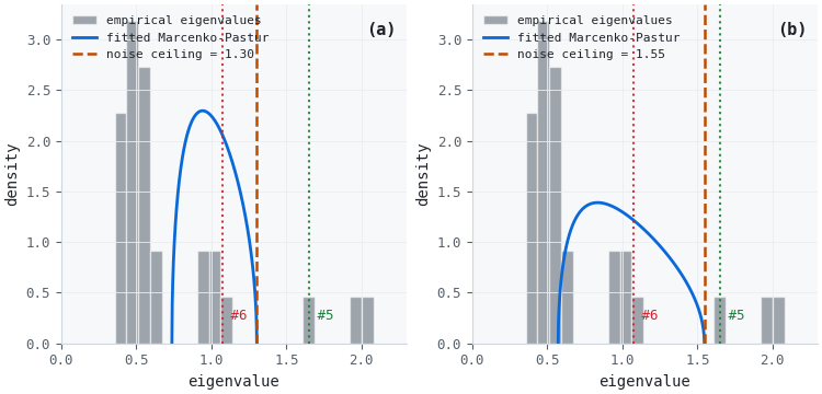
Figure 1. Two-panel illustration of the Marcenko–Pastur fit

• Panel (a): empirical eigenvalue histogram and fitted density using the raw bar count, with the resulting noise ceiling and the fifth and sixth eigenvalues marked.
• Panel (b): the same fit using the AR(1)-adjusted effective sample size; the ceiling shifts right and the fifth eigenvalue's margin over it narrows visibly.

Cluster Recovery, Before and After

With nfacts fixed at five (the effective-sample-size result), the raw correlation matrix is denoised with the constant residual eigenvalue method and then detoned against the first eigenvector. Both the raw and the cleaned matrix are then clustered with the base stage of the ONC algorithm: K-means on the correlation-implied distance √((1 − ρ)/2), sweeping the candidate cluster count and selecting the value that maximizes the silhouette t-statistic.

def cluster_kmeans_base(corr, max_clusters=10, n_init=10, seed=42):
    dist = ((1 - corr) / 2.0) ** 0.5
    best_score, best_labels, best_k = -np.inf, None, None
    for k in range(2, max_clusters + 1):
        labels = KMeans(n_clusters=k, n_init=n_init, random_state=seed).fit_predict(dist)
        silh = silhouette_samples(dist, labels)
        score = silh.mean() / silh.std() if silh.std() > 0 else silh.mean()
        if score > best_score:
            best_score, best_labels, best_k = score, labels, k
    return best_labels, best_k

The full ONC algorithm additionally re-clusters any group whose silhouette quality falls below the average, a redo stage this base version omits; that complete version, tested against MLAM's own reference implementation, is what afml.clustering.onc.get_onc_clusters already provides and what production code should call. The comparison below is between the two correlation matrices, not between clustering algorithms, so the simpler base stage is sufficient to isolate the effect.

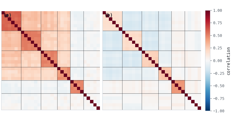
Figure 2. Two-panel illustration of the correlation matrix before and after cleaning

• Panel (a): raw sample correlation, features ordered by true family; block structure is visible but blurred by the shared market-mode tone across families.
• Panel (b): denoised and detoned correlation, same ordering; within-family blocks sharpen and cross-family correlation collapses toward zero.

Clustering on the raw matrix finds only two clusters. One contains every feature from the four market-mode-loaded families (trend, volatility, microstructure, entropy: twenty-one features); the other contains everything without market-mode loading (calendar and noise: nine features). The algorithm is not wrong given its input: with a strong common tone running through most of the panel, family-specific differences are genuinely the smaller signal, and K-means finds the larger one instead. This is the exact failure mode MLAM Section 2.6 describes.

Clustering on the denoised and detoned matrix finds five clusters. Trend, volatility, microstructure, and calendar are each recovered as a single, pure cluster. Entropy is not: it merges with the noise group. That is consistent with 's eigenvalue-margin finding above, entropy was built with the weakest family-specific correlation and its signal eigenvalue barely cleared the noise ceiling in the first place. Detoning removes the market-mode component that had been the only thing making entropy features look distinguishable from noise at all; once that shared tone is gone, what is left of the entropy signal is too weak to separate from the true noise columns under this base clustering stage.

	Raw correlation	Denoised + detoned
Clusters found (k)	2	5
Adjusted Rand Index vs. true families	0.23	0.83

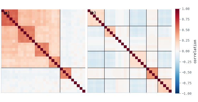
Figure 3. Two-panel illustration of cluster recovery

• Panel (a): raw correlation reordered by its own two-cluster assignment; the market-mode-loaded families are indistinguishable from one another.
• Panel (b): denoised and detoned correlation reordered by its five-cluster assignment; four of five signal families are recovered as pure blocks.

An Adjusted Rand Index of 0.83 against six true groups, with one weak family absorbed into noise, is a more honest result than a contrived perfect recovery would be, and it is the result clustered MDI and MDA in the next article will actually be built on.

Practical Considerations

• Kernel bandwidth sensitivity: the MP fit's bandwidth was fixed at 0.15 in eigenvalue units throughout this article. Refitting it via cross-validation, as MLAM Section 2.8 suggests as an exercise, is worth doing once on a real panel rather than assumed transferable across panels of very different size.
• Effective sample size is a diagnostic, not a certainty: the AR(1) approximation used here is a first-order correction. Features with more complex serial structure (long-memory processes, regime-dependent persistence) will not be fully captured by a single lag-1 autocorrelation coefficient, and the resulting Teff should be read as a more defensible estimate than raw bar count, not an exact one.
• Re-fitting cadence: correlation structure among engineered features is not stationary across regimes. A denoising and clustering pass fit once on a multi-year window and never revisited will drift out of date; this pipeline is a research-time step to be re-run on a rolling or walk-forward basis, not a one-time calibration.
• Market-component count: fixed at one for this single-instrument panel. Multi-instrument panels need this checked, not assumed.

Conclusion

Raw sample correlation among engineered features carries two distinguishable problems: estimation noise, which the Marcenko–Pastur fit separates from signal, and a shared market-mode component, which detoning removes once denoising has identified what counts as signal in the first place. On a representative feature panel built to mirror the production feature set, clustering on the raw correlation matrix collapsed four distinct feature families into a single block driven by their shared market exposure; clustering on the denoised and detoned matrix recovered four of five signal families cleanly, with the weakest family absorbed into the noise cluster rather than falsely separated. The Marcenko–Pastur fit itself is sensitive to an assumption neither AFML nor MLAM makes explicit: that the sample size used in the fit reflects independent observations, which raw bar counts on serially correlated FX bars do not.

The next article uses the cluster assignment produced here as the input to clustered MDI and MDA, compared directly against the naive per-feature MDI, MDA, and SFI methods from AFML Chapter 8 on the same panel, closing the prerequisite named back in Part 9.

Attached Files

File	Location	Description
denoising_detoning.py	afml/denoising/denoising_detoning.py	Marcenko–Pastur eigenvalue fitting, effective sample size correction, constant-residual denoising, and market-mode detoning for correlation matrices. New module created to isolate the denoising/detoning pipeline.
onc.py	afml/clustering/onc.py	Optimal Number of Clusters algorithm. Performs deterministic KMeans base clustering, evaluates silhouette-based cluster quality, and improves below-average clusters recursively. Fixes lazy map evaluation and adds reproducible random state handling.
feature_clusters.py	afml/clustering/feature_clusters.py	Creates clustered feature subsets using ONC or hierarchical linkage. Checks for low-silhouette features and applies multicollinearity transformation via residualization.
codependence_matrix.py	afml/codependence/codependence_matrix.py	Generates dependence and distance matrices from a feature panel using information variation, mutual information, distance correlation, Spearman's rho, GPR, or GNPR methods.
correlation.py	afml/codependence/correlation.py	Implements correlation-based distances: angular, absolute angular, squared angular, and distance correlation.
gnpr_distance.py	afml/codependence/gnpr_distance.py	Provides Spearman's rho, GPR distance, and GNPR distance for copula-based dependence estimation.
information.py	afml/codependence/information.py	Calculates mutual information and variation of information using optimal bin count selection.