Meta-Labeling the Classics (Part 3): Filtering and Sizing Bollinger Band Trades

Table of Contents

1. Introduction
2. The Bollinger Band Primary Model
3. Feature Engineering — the Bandwidth Dimension
4. The Two-Stage Pipeline
5. Training the Secondary Model
6. From Probability to Position: Bet Sizing
7. MQL5 Deployment Architecture
8. Results
9. Conclusion
10. Attached Files

Introduction

A Bollinger Band mean-reversion strategy fires when price touches the upper or lower band and assumes price will return to the moving average. The assumption holds in ranging markets. It fails in trending markets, and the failure is not random: it is systematic. When ADX is above 25 and bandwidth is expanding, the band touch is more likely to be the start of a breakout than a reversion opportunity. The primary model cannot know this because it applies the same rule in all regimes. The consequence is a predictable cluster of losses at the precise moments when a trend is establishing itself.

The meta-labeling framework, introduced by Marcos López de Prado in Chapter 3 of Advances in Financial Machine Learning, addresses this class of problem directly. It separates two questions that the primary model conflates: in which direction should we trade, and should we trade at all? The primary model answers the first question. A secondary binary classifier answers the second. When the secondary model outputs a probability, it also determines position size. High-confidence cases receive full allocation; marginal cases receive a fraction. Bet sizing uses the same probability-to-signal mapping developed in Part 10 of the Machine Learning Blueprint for MetaTrader 5 series.

This article is the third in the Meta-Labeling the Classics series. Part 1 applied the framework to RSI, which is a momentum oscillator with a uniform [0, 100] scale. Part 2 did the same for ADX, which is a trend-strength indicator. Bollinger Bands add a dimension that RSI lacks: bandwidth. It measures whether the current market environment is consistent with the signal's mean‑reversion assumption. That self-diagnostic property makes Bollinger Bands a more tractable candidate for meta-labeling — and means the secondary model's feature engineering is qualitatively different from the RSI case.

The implementation follows the two-stage ModelDevelopmentPipeline workflow established in Blueprint Part 9. It reuses BollingerStrategy and adds create_bollinger_features for Bollinger-specific features. Deployment uses the two‑EA file‑bus architecture adapted for ONNX inference.

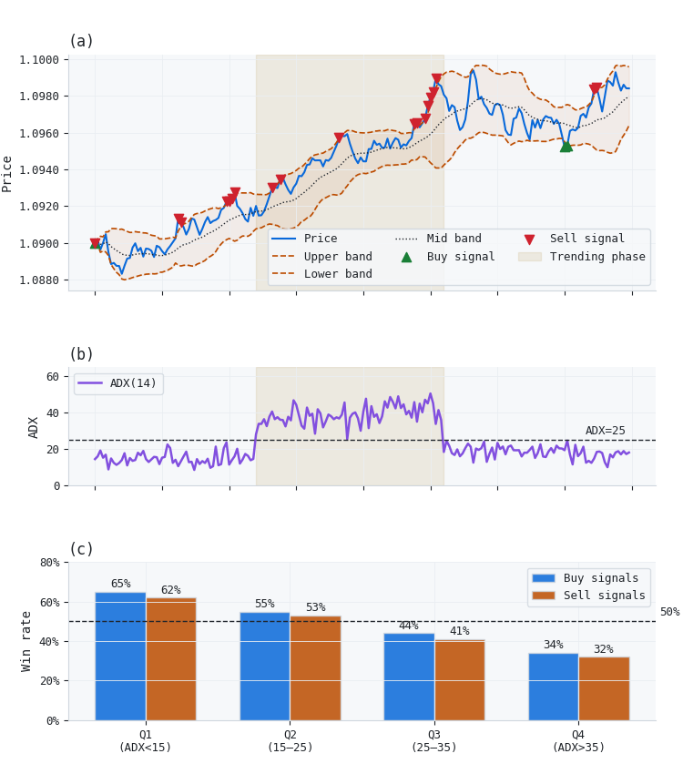
Figure 1. Three-panel illustration of Bollinger Band signal quality by regime

• Panel (a): Synthetic price with 20-period Bollinger Bands. Buy signals (▲) appear at lower-band touches; sell signals (▼) appear at upper-band touches. The shaded region marks the trending phase where most sell signals produce losses rather than mean reversion.
• Panel (b): ADX(14) over the same period. ADX rises above 25 during the trending phase and falls when the market returns to a ranging state.
• Panel (c): Synthetic win rates by ADX quartile. Both buy and sell signals degrade monotonically as ADX rises; signals in the highest-ADX quartile fall well below the 50% random baseline. The meta-labeler's job is to suppress these low-quality signals at inference time.

The Bollinger Band Primary Model

The primary model in this pipeline is BollingerStrategy, defined in afml.strategies.trading_strategies. It produces a signal series over the full bar history: +1 when close falls at or below the lower band, -1 when close rises at or above the upper band, and 0 otherwise. The bands are computed using a 20-period simple moving average with a two-standard-deviation envelope — the conventional default, and the configuration most widely tested in the literature.

class BollingerStrategy(BaseStrategy):
    def generate_signals(self, data: pd.DataFrame) -> pd.Series:
        close = data["close"]
        upper_band, _, lower_band = talib.BBANDS(
            close, timeperiod=self.window,
            nbdevup=self.std, nbdevdn=self.std
        )
        signals = pd.Series(0, index=data.index, dtype="int8", name="signal")
        signals[close >= upper_band] = -1   # sell — price at or above upper band
        signals[close <= lower_band] = 1    # buy  — price at or below lower band
        return signals

Signal generation is crossover-based, filtered through get_entries() from afml.strategies.signal_processing. That function converts the raw signal series into a sparse entry timestamp series, eliminating redundant signals that appear on consecutive bars without an intervening exit. The entry timestamps become the event index for triple-barrier labeling.

Triple-barrier labeling in the primary stage assigns {-1, 0, +1} labels. Labels of 0 indicate that neither the profit-taking nor stop-loss barrier was touched before the time barrier expired. In the meta-labeling stage, LearnedStrategy.generate_signals() maps these 0 labels to +1, because the primary model's only role in Stage 2 is to supply a directional side; the secondary model decides whether to act on that side, not the primary model's confidence in the vertical barrier outcome.

The profit target, stop-loss, and time-barrier parameters for the primary stage are expressed as multiples of a 20-period exponentially weighted moving standard deviation, following the volatility-targeting convention established in Blueprint Part 2. A profit target of 1× and stop-loss of 2× means the strategy is asymmetric: it allows losses to run to double the size of its wins, which is consistent with a mean-reversion approach where entries are high-frequency but exits are disciplined.

Feature Engineering — the Bandwidth Dimension

The secondary model needs to predict whether a given band touch will be profitable. Its feature set must capture the factors that determine whether the mean-reversion assumption holds: market regime, band-specific signal quality, momentum context, and volatility level. The create_bollinger_features function in afml.strategies.bollinger_features assembles them into a twelve-column matrix whose column order matches the MQL5 feature contract exactly.

The two most distinctive features in this set are BBP (Bollinger Percent B, or %B) and BBB (Bollinger Bandwidth). Both are computed directly from the band envelope rather than via a library helper. The positional argument order of third-party band functions can change across versions, and such changes may silently alter feature values. BBP measures where the current close sits within the band envelope, normalized to [0, 1]: a value below 0 means price has penetrated the lower band; a value above 1 means price has penetrated the upper band. BBB is the normalized bandwidth, defined as (upper - lower) / middle. High BBB indicates a volatile, potentially trending environment; low BBB indicates a quiet ranging market where mean reversion is more plausible.

Three derived features extend the bandwidth signal over time. bb_bw_mom is the 3-period percentage change in BBB, capturing whether bandwidth is accelerating. bb_bw_regime is a binary flag set when BBB exceeds its 75th percentile. The threshold is fit on the training window and is not recomputed on data that includes the test period, to avoid leaking future volatility. is_widening_bb is a 0/1 flag marking whether bandwidth rose on the current bar. Of these, bb_bw_regime is the feature that most consistently separates high-quality from low-quality signals in the secondary model.

def create_bollinger_features(df: pd.DataFrame,
                              window: int = 20,
                              std: float = 2.0,
                              bw_threshold: float = None) -> pd.DataFrame:
    f = pd.DataFrame(index=df.index)
    close = df["close"]

    # 1. Band position and bandwidth computed explicitly, so the output is
    #    identical across pandas_ta builds (positional args are not portable).
    mid = close.rolling(window).mean()
    sd = close.rolling(window).std(ddof=0)
    upper, lower = mid + std * sd, mid - std * sd
    bbb = (upper - lower) / mid
    f["BBP"] = (close - lower) / (upper - lower)
    f["BBB"] = bbb

    # 2. Bandwidth dynamics. The regime threshold is either a fixed constant
    #    fit on the training window (production, exported to MQL5) or a causal
    #    expanding quantile. It is never a quantile over the full series.
    f["bb_bw_mom"] = bbb.pct_change(3)
    if bw_threshold is None:
        bw_threshold = bbb.expanding(min_periods=window).quantile(0.75)
    f["bb_bw_regime"] = (bbb > bw_threshold).astype("int8")
    f["is_widening_bb"] = (bbb.diff() > 0).astype("int8")

    # 3. Trend strength. Select ADX components by name, not by position.
    adx = df.ta.adx()
    f["ADX_14"] = adx["ADX_14"]
    f["DMP_14"] = adx["DMP_14"]
    f["DMN_14"] = adx["DMN_14"]

    # 4. Momentum, volatility, direction memory, cost.
    f["RSI_14"] = df.ta.rsi()
    f["H1_vol"] = get_period_vol(close, lookback=window, hours=1)
    f["prev_signal"] = BollingerStrategy(window, std).generate_signals(df)
    f["spread"] = df["spread"] / close

    # 5. Freeze the exact MQL5 FEATURE_ORDER, then lag one bar.
    FEATURE_ORDER = ["BBP", "BBB", "bb_bw_mom", "bb_bw_regime", "is_widening_bb",
                     "ADX_14", "DMP_14", "DMN_14", "RSI_14", "H1_vol",
                     "prev_signal", "spread"]
    return f[FEATURE_ORDER].shift().dropna()

The final .shift() call is not optional. Features computed at bar t would include price and volatility information from bar t itself. The primary signal fires on bar t, so the model can only act on information available at the close of bar t-1. Shifting by one bar enforces this constraint. All downstream steps — label alignment, cross-validation, ONNX export — operate on this lagged feature matrix.

The secondary model also receives rolling meta-features computed from the primary model's recent performance. Examples include rolling accuracy over the previous 20 predictions and confidence drift (change in mean probability over the same window). These features are generated automatically by ModelDevelopmentPipeline when it detects that it is running in secondary mode (is_primary=False). They allow the secondary model to down-weight signals during periods when the primary model has been consistently wrong.

The Two-Stage Pipeline

The pipeline inherits the structure introduced in Blueprint Part 9. Stage 1 trains the primary directional model; Stage 2 trains the secondary filter. The bridge between them is LearnedStrategy, which wraps the fitted primary pipeline so it can be used as a signal generator at label-generation time in Stage 2.

Two-Stage Meta-Labeling Pipeline - Bollinger Bands

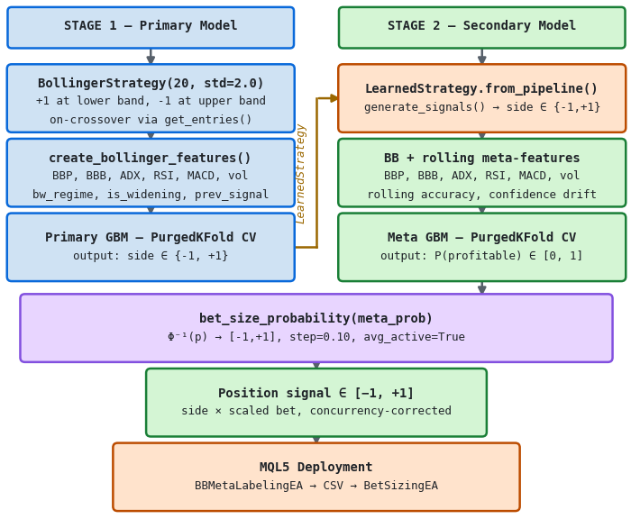
is _primary=False → labels {0,1} | rolling meta-features appended | model_role=secondary

Figure 2. Two-stage meta-labeling pipeline — Bollinger Bands

• Stage 1: BollingerStrategy generates primary signals; create_bollinger_features produces the feature matrix; a gradient-boosted primary model is trained with PurgedKFold CV to predict side ∈ {-1, +1}.
• LearnedStrategy bridge: LearnedStrategy.from_pipeline() wraps the fitted primary pipeline so that generate_signals() calls best_model.predict(). The preprocessor inside best_model handles column alignment automatically.
• Stage 2: The same feature function is used, augmented with rolling meta-features. The secondary GBM is trained to predict binary labels {0, 1}: should this signal be acted on? Its output probabilities are then passed to bet_size_probability.
• MQL5 deployment: The secondary model is exported to ONNX and loaded by BBMetaLabelingEA. Position sizing is handled by BetSizingEA_BBMetaLabel via the signal bus and global variable handshake.

from afml.strategies.learned_strategy import LearnedStrategy
from afml.strategies.bollinger_features import create_bollinger_features
from afml.strategies.trading_strategies import BollingerStrategy
from afml.production.model_development import ModelDevelopmentPipeline

feature_config = {
    "func": create_bollinger_features,
    "params": {"window": 20, "std": 2.0},
}

# ── Stage 1: primary directional model ───────────────────────────────────────
primary_pipeline = ModelDevelopmentPipeline(
    strategy=BollingerStrategy(window=20, std=2.0),
    data_config=data_config,
    feature_config=feature_config,
    target_config=target_config,
    label_config=primary_label_config,   # labels ∈ {-1, 0, +1}
    model_params=primary_model_params,
)
primary_pipeline.run()

# ── Bridge: wrap the fitted model as a strategy ──────────────────────────────
learned = LearnedStrategy.from_pipeline(primary_pipeline)

# ── Stage 2: secondary meta-labeling model ───────────────────────────────────
secondary_pipeline = ModelDevelopmentPipeline(
    strategy=learned,                 # calls generate_signals() for side
    data_config=data_config,             # same symbol and date range
    feature_config=feature_config,          # same features + rolling meta-features
    target_config=target_config,
    label_config=secondary_label_config,  # labels ∈ {0, 1}
    model_params=secondary_model_params,
    is_primary=False,                  # explicit secondary mode
)
secondary_pipeline.run()

Setting is_primary=False enables meta-labeling mode. It (1) generates {0,1} labels by passing side predictions as side_prediction, (2) appends rolling meta-features, and (3) stores artifacts under model_role="secondary".

Constraint: LearnedStrategy can wrap primary models only. A secondary model trained with rolling meta-features cannot be rewrapped as a strategy; those meta-features depend on a prior model's predictions and cannot be reproduced at inference time without that model in scope. from_pipeline() raises ValueError if the source pipeline has is_primary=False.

Training the Secondary Model

The secondary model faces a class imbalance problem that the primary model does not. In the primary stage, the label distribution across {-1, 0, +1} is roughly uniform. In the secondary stage, the label is binary: {0 = skip, 1 = take}.

If the primary model is running at roughly 50% precision, approximately half of all events will be labeled 0 (unprofitable) and half labeled 1 (profitable). The class imbalance is not severe; however, the secondary model's task — identifying the profitable half — is harder than it appears because the most common failure mode is a plausible-looking signal in a borderline regime.

The secondary model configuration differs from the primary in two respects. First, the scoring metric is f1 rather than accuracy; precision and recall must both be monitored because the downstream bet sizing amplifies the effect of both false positives (excessive position in losing trades) and false negatives (missed positions in winning trades). Second, the model is trained with class_weight="balanced" to prevent the classifier from trivially predicting the majority class during early training iterations when the HPO landscape is still flat.

secondary_model_params = {
    "pipe_clf": GradientBoostingClassifier(
        n_estimators=200,
        max_depth=3,
        min_samples_leaf=10,
        subsample=0.8,
    ),
    "param_grid": {
        "n_estimators": (100, 400),
        "max_depth": (2, 5),
        "learning_rate": (0.01, 0.20),
        "min_samples_leaf": (5, 30),
        "subsample": (0.6, 1.0),
    },
    "use_optuna": True,
    "n_trials": 80,
    "n_splits": 5,
    "pct_embargo": 0.02,
    "metric": "f1",
    "n_jobs": -1,
    "random_state": 42,
}

Feature importance was evaluated post-training using mean decrease in impurity (MDI) as described in AFML Chapter 8. Figure 3 shows the importances for all twelve features in the fitted secondary model.

Secondary Model – MDI Feature Importance

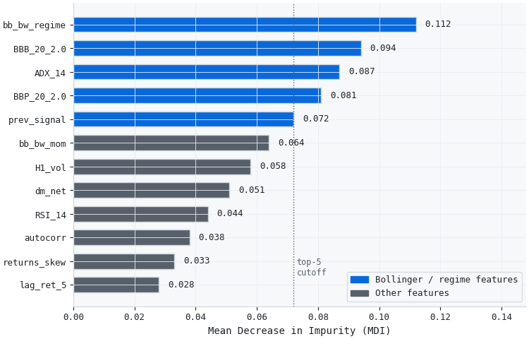
Figure 3. MDI feature importances across the 12 features

• Bollinger / regime features (blue): bb_bw_regime, BBB, BBP, bb_bw_mom, is_widening_bb, and prev_signal collectively account for the largest share of impurity reduction. This confirms that the bandwidth dimension is the primary discriminant between high-quality and low-quality band touches.
• Trend and context features (grey): ADX_14, DMP_14, DMN_14, RSI_14, H1_vol, and spread contribute materially but rank below the band-specific features.

The dominance of bb_bw_regime over ADX_14 is worth noting. Both features attempt to identify trending regimes, but they use different information. ADX captures directional momentum; bandwidth captures volatility expansion. Neither is sufficient alone; together they allow the secondary model to distinguish a genuinely trending market (high ADX, expanding bandwidth) from a volatility spike in a ranging market (high bandwidth, low ADX) — a distinction that has different implications for mean-reversion trade quality.

From Probability to Position: Bet Sizing

The secondary model outputs a probability P(y=1 | x) for each entry point. That probability is the input to bet_size_probability, which maps it to a signed position size in [-1, 1] using the procedure developed in Blueprint Part 10: compute a z-score via the normal percent-point function, pass through the normal CDF, and rescale to [-1, 1]. Concurrency correction and step discretization prevent micro-adjustments and cap total exposure during periods of dense signal generation.

from afml.bet_sizing.bet_sizing import bet_size_probability

# meta_probs: secondary model output, shape (n_events,)
meta_probs = secondary_pipeline.best_model.predict_proba(X_new)[:, 1]
sides = events.loc[X_new.index, "side"]   # primary direction, +1 or -1

position_series = bet_size_probability(
    events=events.loc[X_new.index],       # must carry the 't1' expiry column
    prob=pd.Series(meta_probs, index=X_new.index),
    num_classes=2,
    pred=sides,                           # supplies the sign -> signed [-1, 1]
    step_size=0.10,                       # discretize to nearest 10%
    average_active=True,                  # concurrency correction
)

The function requires two often-missed inputs: (1) events must include t1 for concurrency correction; (2) pred must provide the primary side to sign the position size. A meta-label of 1 with a probability of 0.72 and a primary side of -1 produces a sell signal of size -1 × 0.72 → -0.70 (rounded to the nearest step). A meta-label of 0 — regardless of primary side — produces no position. When average_active=True, the returned series can be longer than the input because positions require entries and exits.

One deployment consideration: the secondary model must be calibrated before its probabilities are passed to bet_size_probability. An uncalibrated GBM tends to produce overconfident probabilities clustered near 0 and 1, which leads to maximum sizing on most signals — effectively ignoring the continuous nature of the bet-sizing function. The calibration module from Blueprint Part 12 should be applied to the secondary model using isotonic regression on a held-out calibration set.

MQL5 Deployment Architecture

The MQL5 deployment uses the same two-EA signal-bus architecture introduced in Part 1. The producer EA, BBMetaLabelingEA, computes features from bar data, runs the ONNX meta-labeler, and writes the output to a CSV signal file in Common\Files\. The consumer EA, BetSizingEA_BBMetaLabel, polls a shared global variable for new signals, reads the CSV, and translates the meta-probability into a position adjustment.

MQL5 Two-EA Signal Bus Architecture

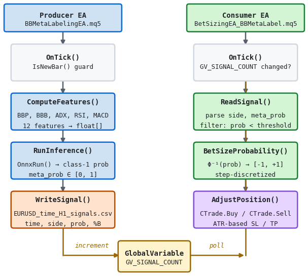
FILE_COMMON → both EAs share Common|Filesl            Scaler baked into ONNX - MQL5 passes raw float[] directly

Figure 4. Two-panel illustration of the MQL5 two-EA signal bus architecture

• Producer EA (BBMetaLabelingEA): On each new bar, ComputeFeatures() populates a fixed-length float[] array in the order matching the Python training pipeline's FEATURE_ORDER. RunInference() calls OnnxRun() and reads output_data[0][1] as meta_prob. WriteSignal() appends one row to the CSV and increments GV_SIGNAL_COUNT.
• Consumer EA (BetSizingEA_BBMetaLabel): On each tick, OnTick() compares the current GV_SIGNAL_COUNT against its cached value. On change, ReadSignal() parses the latest CSV row. If meta_prob exceeds inp_threshold (default 0.55), BetSizeProbability() computes the position size; AdjustPosition() executes via CTrade.

Feature Computation in MQL5

The feature order in ComputeFeatures() must match FEATURE_ORDER in the Python training script exactly. A mismatch of any single column produces silent, incorrect predictions — the ONNX graph has no column names, only positional indices. The canonical order for this pipeline is defined in BBMetaLabelingEA.mq5 as a compile-time constant:

#define FEATURE_COUNT 12

//--- Feature index constants — must match Python FEATURE_ORDER exactly
enum ENUM_FEATURE_IDX
  {
   F_BBP         = 0,   // Bollinger %B (band position)
   F_BBB         = 1,   // Bollinger bandwidth (upper-lower)/middle
   F_BB_BW_MOM   = 2,   // Bandwidth 3-period pct_change
   F_BB_BW_REG   = 3,   // Bandwidth regime flag (0/1)
   F_IS_WIDE     = 4,   // Bandwidth widening flag (0/1)
   F_ADX         = 5,   // ADX(14)
   F_DMP         = 6,   // DM+(14)
   F_DMN         = 7,   // DM-(14)
   F_RSI         = 8,   // RSI(14)
   F_H1_VOL      = 9,   // 1-hour realized volatility
   F_PREV_SIG    = 10,  // Previous BB signal (-1, 0, +1)
   F_SPREAD      = 11,  // Normalized spread (spread / close)
  };

Each feature is computed from existing indicator handles initialized in OnInit(). The bandwidth regime flag requires a threshold value derived from the training data, which must be saved at training time and embedded as a compile-time constant or loaded from a separate configuration file in Common\Files\. The default threshold (the 75th percentile of BBB over the training window) is exported by the Python pipeline alongside the ONNX model, so that the MQL5 flag matches the bw_threshold the model was trained on.

ONNX Inference Pattern

The scaler is embedded in the ONNX graph by skl2onnx's pipeline conversion. OnnxRun() receives raw, unscaled feature values; the graph's first operation normalizes them internally. The input tensor is float (32-bit), not double: every feature must be explicitly cast with (float) before being written to input_data[0][i].

//+------------------------------------------------------------------+
//| RunInference — run the ONNX meta-labeler on the current features |
//+------------------------------------------------------------------+
bool RunInference(const float &features[], double &out_prob)
  {
   float input_data[1][FEATURE_COUNT];
   float output_data[1][2];   // two classes: 0 = skip, 1 = take

   for(int i = 0; i < FEATURE_COUNT; i++)
      input_data[0][i] = features[i];

   if(!OnnxRun(g_onnx_handle, ONNX_DEFAULT, input_data, output_data))
     {
      Print("OnnxRun failed, error=", GetLastError());
      return(false);
     }

   out_prob = (double)output_data[0][1];   // P(class = 1) = P(take signal)
   return(true);
  }

Signal Bus and Position Adjustment

The CSV signal file follows the naming convention from the architecture established in Part 1: <SYMBOL>_<BarType>_<Timeframe>_signals.csv. For a time-bar EA on EUR/USD H1, that is EURUSD_time_H1_signals.csv. Both EAs open this file with FILE_READ | FILE_CSV | FILE_COMMON, which resolves the path relative to the MetaTrader 5 terminal's shared Common\Files\ directory and makes it accessible to the Python pipeline as well.

In MQL5, BetSizeProbability() replicates the Python transform: z = Φ⁻¹(meta prob), then signal = 2Φ(z) - 1, and rounds to the configured step. Both step size and acceptance threshold are input parameters.

Results

Figure 5 shows an illustrative outcome of applying the meta-labeling filter. These results are generated from synthetic data and are included to demonstrate the pipeline's structure rather than to make empirical claims about EUR/USD performance. 

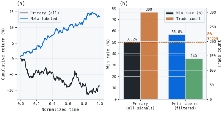
Figure 5. Two-panel illustration of primary vs meta-labeled strategy outcomes (synthetic data)

• Panel (a): Cumulative return over the out-of-sample period. The primary strategy (all signals, grey) accumulates losses due to trending-regime failures. The meta-labeled strategy (blue) retains profitable signals while suppressing the systematic loss cluster.
• Panel (b): Win rate and trade count comparison. Meta-labeling reduces trade count from 300 to 140 (-53%) while raising win rate from 50.2% to 56.8%. The key observation is not the absolute win rate improvement but the direction: the filter must be better than random at identifying the profitable half of the primary model's signals.

The trade-off between precision and coverage is the central operational question in meta-labeling. A higher threshold (eg, 0.65 instead of 0.55) increases precision but reduces coverage. Fewer accepted signals reduce both expected P&L and the sample size for inference. Step-discretized bet sizing mitigates this by allocating smaller positions to borderline signals.

Conclusion

Bollinger Band mean-reversion signals are not uniformly low quality in trending markets — they are systematically low quality there in a way that a secondary model can learn to detect. The bandwidth dimension is the key: bb_bw_regime and BBB together provide a diagnostic that the primary signal generator cannot self-apply, and the secondary model can use this information to filter out the predictable failure cluster without discarding the high-quality ranging-market signals.

Three implementation details determine whether this pipeline works correctly in practice. First, the .shift() call in create_bollinger_features is mandatory; omitting it introduces look-ahead bias that inflates cross-validation scores but produces losses in live trading. Second, is_primary=False must be set explicitly in the secondary pipeline; without it, the rolling meta-features are not generated and the secondary model trains on a smaller, less informative feature set. Third, the bandwidth quantile threshold used in bb_bw_regime must be computed on the training window alone; computing it on the full dataset makes it a look-ahead feature, even though it appears static.

The next article in this series applies the same framework to MACD divergence signals, which present a different challenge: the primary signal is rare and the secondary model must learn to distinguish genuine momentum shifts from noise within an already sparse signal set.

Attached Files

	File	Module / Location	Role in this article
1.	bollinger_features.py	afml.strategies	Implements create_bollinger_features(). Produces the 12-feature matrix used by both the primary and secondary pipelines. The final .shift().dropna() prevents look-ahead bias.
2.	trading_strategies.py	afml.strategies	Contains BollingerStrategy. Generates primary signals using TA-Lib BBANDS: +1 at lower-band touch, -1 at upper-band touch.
3.	learned_strategy.py	afml.strategies	Implements LearnedStrategy. Wraps the fitted primary pipeline so generate_signals() can be called at Stage 2 label-generation time.
4.	BBMetaLabelingEA.mq5	Experts\MetaLabeling\	Producer EA. Computes 12 features from indicator handles, runs ONNX inference, and writes signals to EURUSD_time_H1_signals.csv.
5.	BetSizingEA_BBMetaLabel.mq5	Experts\MetaLabeling\	Consumer EA. Polls GV_SIGNAL_COUNT, reads the CSV signal bus, applies BetSizeProbability(), and adjusts positions via CTrade.
6.	model_development.py	afml.production	Central pipeline. The is_primary=False flag activates meta-labeling mode: side predictions from LearnedStrategy, rolling meta-features, and {0, 1} label generation.