

The Deflated Sharpe Ratio in MQL5: Telling a Real Edge from a Lucky Backtest
 92
92
 0
0

Contents
- The Sharpe ratio that flatters a backtest
- The three reasons a raw Sharpe ratio is optimistic
- The Probabilistic Sharpe Ratio
- The deflated benchmark for the number of trials
- The class from scratch
- The best of 56 backtests
- Two controls with a known answer
- Files and how to run it
- Limitations
- Conclusion
The Sharpe ratio that flatters a backtest
You optimize a strategy. You review the results, and one variant stands out with a convincing Sharpe ratio. You publish it, or you trade it, and it does not hold. Nothing was faked. The backtest was real and the number was computed correctly. It still overstated the evidence, because a Sharpe ratio read off the best of many runs is biased upward by the selection itself.
This site already has articles about the ratio and about the risk of trusting one backtest. The article Mathematics in trading: Sharpe and Sortino ratios explains how the ratio is calculated and notes that it assumes normally distributed returns. The article Rolling Sharpe Ratio with Statistical Significance Bands in MQL5 plots a rolling Sharpe ratio of the bar returns with significance bands. The bands use Andrew Lo's standard error for independent, normally distributed returns. The article Hypothesis Testing for Trading Strategies builds a one-sample t-test in MQL5 for whether the mean return differs from 0. The article Stress Testing Trade Sequences with Monte Carlo in MQL5 resamples the trade results to build equity paths, a drawdown distribution and a probability of ruin.
Three more articles deal with the search itself. The article Combinatorially Symmetric Cross Validation In MQL5 estimates the probability of backtest overfitting from the bar-by-bar returns of every optimization pass. The article Unified Validation Pipeline Against Backtest Overfitting combines that method with other cross-validation methods in Python, and lists the Deflated Sharpe Ratio paper as further reading. The article From "Best Pass" to Robust Solutions: Exploring the Optimization Surface in MetaTrader 5 exports the metrics of every pass and looks for a stable plateau around the best pass.
None of these articles computes the Probabilistic Sharpe Ratio or the Deflated Sharpe Ratio. The first four work on one series of returns or trade results at a time and do not count how many variants were tried. The last three look at the whole search, but they do not give a probability for the Sharpe ratio of the selected variant. This article adds that calculation, and it complements those checks. It needs only the trade returns of the winner and one Sharpe ratio per variant.
Both ratios are implemented in one small native class. The Probabilistic Sharpe Ratio (PSR) accounts for sample length and the shape of the return distribution. The Deflated Sharpe Ratio (DSR) also accounts for the number of variants searched, which is the adjustment that applies when a result was picked during optimization. The class implements the moments, the normal distribution and its inverse itself, so it needs no Python, no DLL and no include file.
This is a technical and educational article, not a strategy and not financial advice. It delivers a reusable measurement for reading your own backtests.
The three reasons a raw Sharpe ratio is optimistic
The Sharpe ratio is the mean of returns divided by their standard deviation. As a number it is fine. As evidence of an edge it is optimistic for three separate reasons, and it helps to name them, because different adjustments handle different ones.
The first is sample length. A Sharpe ratio measured over 40 trades is a much noisier estimate than the same value measured over 400 trades, and the raw number does not tell you which one you have.
The second is the shape of the returns. Trading returns are rarely distributed as the bell curve that the textbook formula assumes. They are skewed and fat-tailed: many small winners and a few large losers, or the reverse. That shape changes how uncertain the ratio is, and the plain formula ignores it.
The third is selection. If you try 50 parameter sets and keep the best Sharpe ratio, that best value is biased upward by the search. The largest of many noisy estimates overstates, on average, the true value of the variant that produced it, even when none of the strategies has an edge.
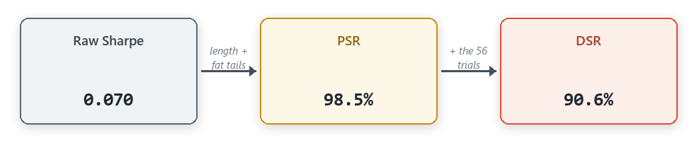
A raw Sharpe ratio ignores all three problems. The PSR accounts for sample length and the shape of the returns. The DSR also accounts for how many variants were tried, which is the adjustment for the bias of picking the winner. The values are those of the market example in the section The best of 56 backtests.
The first two are handled by the PSR. The third needs the DSR on top of it.
The Probabilistic Sharpe Ratio
The Probabilistic Sharpe Ratio was introduced by Bailey and Lopez de Prado in the paper "The Sharpe Ratio Efficient Frontier" (2012). It does not report a Sharpe ratio. It reports a probability: the probability that the true Sharpe ratio is above a chosen benchmark, given the sample. Instead of asking how large the ratio is, it asks how confident the data lets you be that the ratio is above the benchmark.
It uses the higher moments of the returns directly. The observed Sharpe ratio, the number of observations, the skewness and the kurtosis go into one expression whose output is a probability between 0 and 1. When the sample is long and close to normal, a modest Sharpe ratio can be highly significant. When the sample is short, a large Sharpe ratio can still fail to reach 95 percent.
To evaluate it you need the standard normal cumulative distribution function (CDF), the probability that a standard normal draw falls below a given value. The Standard Library provides one, MathCumulativeDistributionNormal, in Math\Stat\Normal.mqh. This class is meant to work as a single file with no includes, so it computes the distribution itself with a rational approximation of the error function. Its absolute error is below 0.000001, which is sufficient here.
//+------------------------------------------------------------------+
//| Standard normal CDF via a rational approximation of erf          |
//+------------------------------------------------------------------+
double CDeflatedSharpe::NormalCDF(const double z)
  {
   double x = z / MathSqrt(2.0);
   int    sign = (x < 0.0) ? -1 : 1;
   x = MathAbs(x);
   double t = 1.0 / (1.0 + 0.3275911 * x);
   double y = 1.0 - (((((1.061405429 * t - 1.453152027) * t) + 1.421413741) * t
                      - 0.284496736) * t + 0.254829592) * t * MathExp(-x * x);
   double erf = sign * y;
   return(0.5 * (1.0 + erf));
  }
The PSR itself is a direct translation of the formula. It takes the return series and a benchmark Sharpe ratio, computes the observed Sharpe ratio and the two higher moments, and returns the probability.
The kurtosis in this formula is Pearson kurtosis, on which a normal distribution scores 3. It is not excess kurtosis, on which a normal distribution scores 0. In the code g4 holds the Pearson value, which is why the term reads (g4 - 1) / 4. Written with excess kurtosis, the same term would be (excess kurtosis + 2) / 4. Both the skewness and the kurtosis are standardized with the sample standard deviation, the one that divides by n - 1.
//+------------------------------------------------------------------+
//| Probabilistic Sharpe Ratio: P(true Sharpe ratio > srStar)        |
//| Accounts for sample length, skewness and Pearson kurtosis        |
//| (normal = 3, not excess kurtosis).                               |
//+------------------------------------------------------------------+
double CDeflatedSharpe::PSR(const double &r[], const double srStar = 0.0)
  {
   int n = ArraySize(r);
   if(n < 4)
      return(0.0);
   double sr = Sharpe(r);
   double g3 = Skew(r);
   double g4 = Kurtosis(r);            // Pearson kurtosis (normal = 3), not excess kurtosis
   double denom = 1.0 - g3 * sr + ((g4 - 1.0) / 4.0) * sr * sr;
   if(denom <= 0.0)
      return(0.0);
   double z = (sr - srStar) * MathSqrt((double)(n - 1)) / MathSqrt(denom);
   return(NormalCDF(z));
  }
The skewness enters the denominator with a negative sign, multiplied by the Sharpe ratio. For a positive Sharpe ratio, negative skewness makes the ratio less certain. This is the long left tail of a strategy with many small gains and a few large losses. Positive skewness does the opposite. Higher kurtosis adds uncertainty. With a benchmark of 0 the result is the probability that the true Sharpe ratio is positive.
The deflated benchmark for the number of trials
The PSR judges one strategy in isolation. If you optimized 50 variants and passed it the best one, it reports that one as significant, because it has no information about the other 49.
The Deflated Sharpe Ratio comes from a later paper by the same authors, "The Deflated Sharpe Ratio: Correcting for Selection Bias, Backtest Overfitting and Non-Normality" (2014). It handles the search by raising the benchmark. Instead of testing against 0, it tests against the Sharpe ratio expected from the best of the trials when none of them has an edge. If you try enough strategies with no edge, the best of them still shows a positive Sharpe ratio, and that expected maximum can be estimated. This article calls that expected maximum the hurdle. It depends on the number of trials and on the dispersion of their Sharpe ratios. It also needs the inverse of the normal CDF, the quantile function, which the PSR does not use.
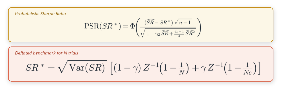
The PSR turns the observed Sharpe ratio, the sample size and the higher moments into a probability. The deflated benchmark is the Sharpe ratio expected from the best of N trials with no edge. The DSR is the PSR measured against that benchmark.
In both formulas SR with a hat is an observed Sharpe ratio, SR with a star is the benchmark, and the capital phi is the standard normal CDF. In the first formula n is the number of trades of the series, gamma 3 is its skewness and gamma 4 is its Pearson kurtosis. In the code they are g3 and g4. In the second formula N is the number of trials and k is the index of a trial. The variance is taken across the observed Sharpe ratios of those N trials. The gamma without a subscript is the Euler-Mascheroni constant, and e is Euler's number, 2.718.
In code the expected maximum is a short function. It takes the variance of the Sharpe ratios across the trials and the number of trials. It combines two normal quantiles with the Euler-Mascheroni constant, which is a standard approximation for the expected maximum of N independent normal draws.
//+------------------------------------------------------------------+
//| Expected maximum Sharpe ratio of nTrials independent strategies  |
//| with no edge, given the variance of their Sharpe ratios. With    |
//| correlated or structurally different trials it is an             |
//| approximation.                                                   |
//+------------------------------------------------------------------+
double CDeflatedSharpe::ExpectedMaxSharpe(const double varSR, const int nTrials)
  {
   if(nTrials <= 1 || varSR <= 0.0)
      return(0.0);
   double emc = 0.5772156649015329;      // Euler-Mascheroni constant
   double e   = 2.718281828459045;
   double q1  = NormalInv(1.0 - 1.0 / nTrials);
   double q2  = NormalInv(1.0 - 1.0 / (nTrials * e));
   return(MathSqrt(varSR) * ((1.0 - emc) * q1 + emc * q2));
  }
The variance input needs a precise definition, because the hurdle is proportional to its square root. In this article varSR is the sample variance of the observed Sharpe ratios of all the variants that were tried, the winner included. Every Sharpe ratio in that sample is the per-trade, non-annualized value that the class returns, computed on the same price history. The variance divides by N - 1. The paper defines this input as the variance across the estimated Sharpe ratios of the trials, and it assumes that the trials are independent. It does not state the divisor. With 56 trials, dividing by N instead would move the hurdle from 0.0279 to 0.0276.
That is a practical approximation, not an exact estimate of a theoretical variance. The observed spread mixes two things: real differences between the variants, and the estimation noise of each Sharpe ratio. The formula also treats the trials as independent draws from one distribution. With strongly correlated variants, such as neighboring lookback periods, or with structurally different strategies, the hurdle is approximate. It is an estimate and should not be read as a canonical value.
The hurdle is also measured from 0. It is the expected maximum under the hypothesis that no variant has an edge. It equals the standard deviation of the trial Sharpe ratios multiplied by a factor that depends only on the number of trials. For 56 trials that factor is 2.32. The hurdle is not centered on the average of the observed ratios. When the variants share a common component, as lookback periods of one strategy on one price series do, many of them can be above the hurdle at the same time.
The DSR is then the PSR measured against that raised benchmark instead of against 0. In code it takes two lines: one computes the hurdle and the other calls PSR with it. The result is read as the confidence that the Sharpe ratio of the winner is more than the best of that many trials with no edge would show.
//+------------------------------------------------------------------+
//| Deflated Sharpe Ratio: PSR of the best series against the        |
//| expected-maximum benchmark for nTrials. varSR is the sample      |
//| variance of the observed Sharpe ratios of all trials, the best   |
//| one included: a practical estimate, not an exact value.          |
//+------------------------------------------------------------------+
double CDeflatedSharpe::DSR(const double &rBest[], const double varSR, const int nTrials)
  {
   double srStar = ExpectedMaxSharpe(varSR, nTrials);
   return(PSR(rBest, srStar));
  }
The class from scratch
The class has only static methods, so any of them can be called without creating an object. The moments feed the significance tests. The normal distribution and its inverse make the probabilities computable. The results built on them are the Sharpe ratio, the PSR, the hurdle and the DSR.
//+------------------------------------------------------------------+
//| Probabilistic and Deflated Sharpe Ratio, from scratch            |
//+------------------------------------------------------------------+
class CDeflatedSharpe
  {
public:
   //--- sample moments of a return series
   static double     Mean(const double &x[]);           // arithmetic mean
   static double     Std(const double &x[]);            // sample standard deviation (divides by n - 1)
   static double     Skew(const double &x[]);           // skewness, third standardized moment
   static double     Kurtosis(const double &x[]);       // Pearson kurtosis, normal = 3

   //--- native normal distribution
   static double     NormalCDF(const double z);         // standard normal cumulative probability
   static double     NormalInv(const double p);         // inverse of the standard normal CDF

   //--- Sharpe ratio and its significance
   static double     Sharpe(const double &r[]);         // observed Sharpe ratio, per observation, not annualized
   static double     PSR(const double &r[], const double srStar = 0.0);                 // Probabilistic Sharpe Ratio against a benchmark
   static double     ExpectedMaxSharpe(const double varSR, const int nTrials);          // deflation hurdle for nTrials
   static double     DSR(const double &rBest[], const double varSR, const int nTrials); // Deflated Sharpe Ratio
  };
The moments are ordinary sums. The standard deviation is the sample one, which divides by n - 1. The Sharpe ratio is the mean divided by that standard deviation. It is a per-observation value: with one return per trade it is a per-trade Sharpe ratio, and it is not annualized.
//+------------------------------------------------------------------+
//| Sample standard deviation (divides by n - 1)                     |
//+------------------------------------------------------------------+
double CDeflatedSharpe::Std(const double &x[])
  {
   int n = ArraySize(x);
   if(n < 2)
      return(0.0);
   double m = Mean(x);
   double s = 0.0;
   for(int i = 0; i < n; i++)
      s += (x[i] - m) * (x[i] - m);
   return(MathSqrt(s / (n - 1)));
  }
//+------------------------------------------------------------------+
//| Observed Sharpe ratio of a return series: mean divided by the    |
//| sample standard deviation, per observation, not annualized       |
//+------------------------------------------------------------------+
double CDeflatedSharpe::Sharpe(const double &r[])
  {
   double sd = Std(r);
   if(sd == 0.0)
      return(0.0);
   return(Mean(r) / sd);
  }
The skewness and the kurtosis standardize each return with that mean and that standard deviation. Kurtosis is the fourth standardized moment on the Pearson scale, where a normal distribution scores 3. This is the convention the PSR formula expects. Skew follows the same pattern with the third power, and Mean is a plain average. Both are in the attached file.
//+------------------------------------------------------------------+
//| Kurtosis (fourth standardized moment, normal distribution = 3)   |
//+------------------------------------------------------------------+
double CDeflatedSharpe::Kurtosis(const double &x[])
  {
   int n = ArraySize(x);
   if(n < 4)
      return(3.0);
   double m = Mean(x);
   double sd = Std(x);
   if(sd == 0.0)
      return(3.0);
   double s = 0.0;
   for(int i = 0; i < n; i++)
     {
      double z = (x[i] - m) / sd;
      s += z * z * z * z;
     }
   return(s / n);
  }
The last piece is the inverse normal, the quantile function. It turns a probability back into the value that a standard normal variable stays below with that probability. The Standard Library provides it as MathQuantileNormal in the same include file. The class uses Acklam's rational approximation instead, with a relative error of about 0.000000001. The deflated benchmark calls it twice.
//+------------------------------------------------------------------+
//| Inverse standard normal CDF (Acklam's rational approximation)    |
//+------------------------------------------------------------------+
double CDeflatedSharpe::NormalInv(const double p)
  {
   if(p <= 0.0)
      return(-1.0e10);
   if(p >= 1.0)
      return(1.0e10);
   double a1 = -3.969683028665376e+01, a2 =  2.209460984245205e+02;
   double a3 = -2.759285104469687e+02, a4 =  1.383577518672690e+02;
   double a5 = -3.066479806614716e+01, a6 =  2.506628277459239e+00;
   double b1 = -5.447609879822406e+01, b2 =  1.615858368580409e+02;
   double b3 = -1.556989798598866e+02, b4 =  6.680131188771972e+01;
   double b5 = -1.328068155288572e+01;
   double c1 = -7.784894002430293e-03, c2 = -3.223964580411365e-01;
   double c3 = -2.400758277161838e+00, c4 = -2.549732539343734e+00;
   double c5 =  4.374664141464968e+00, c6 =  2.938163982698783e+00;
   double d1 =  7.784695709041462e-03, d2 =  3.224671290700398e-01;
   double d3 =  2.445134137142996e+00, d4 =  3.754408661907416e+00;
   double plow = 0.02425, phigh = 1.0 - 0.02425;
   double q, r;
   if(p < plow)
     {
      q = MathSqrt(-2.0 * MathLog(p));
      return((((((c1 * q + c2) * q + c3) * q + c4) * q + c5) * q + c6) /
             ((((d1 * q + d2) * q + d3) * q + d4) * q + 1.0));
     }
   if(p > phigh)
     {
      q = MathSqrt(-2.0 * MathLog(1.0 - p));
      return(-(((((c1 * q + c2) * q + c3) * q + c4) * q + c5) * q + c6) /
             ((((d1 * q + d2) * q + d3) * q + d4) * q + 1.0));
     }
   q = p - 0.5;
   r = q * q;
   return((((((a1 * r + a2) * r + a3) * r + a4) * r + a5) * r + a6) * q /
          (((((b1 * r + b2) * r + b3) * r + b4) * r + b5) * r + 1.0));
  }
The best of 56 backtests
A formula is convincing when you see it flag a false positive. The demo has two steps. The first is a market example, where the true answer is unknown. The second is a pair of synthetic controls, where it is known.
The market example does what an optimization does. It sweeps a simple moving-average strategy across every lookback period from 5 to 60, one trial per period, and keeps the variant with the highest Sharpe ratio. The strategy is long above its average and short below it, and it books a return on every flip.
//+------------------------------------------------------------------+
//| Run one moving-average strategy and collect its per-trade        |
//| returns. Long when price is above its average, short when below; |
//| a return is booked on every flip. Returns the number of trades.  |
//+------------------------------------------------------------------+
int RunVariant(const double &price[], const int period, double &ret[])
  {
   ArrayResize(ret, 0);
   int bars = ArraySize(price);
   if(bars <= period + 2)
      return(0);

   int    pos = 0;            // +1 long, -1 short, 0 flat
   double entry = 0.0;
   for(int i = period; i < bars - 1; i++)
     {
      double ma = 0.0;
      for(int k = 0; k < period; k++)
         ma += price[i - k];
      ma /= period;

      int want = (price[i] > ma) ? 1 : -1;
      if(want != pos)
        {
         if(pos != 0)
           {
            double r = pos * (price[i] - entry) / entry;   // return of the closed trade
            int n = ArraySize(ret);
            ArrayResize(ret, n + 1);
            ret[n] = r;
           }
         pos = want;
         entry = price[i];
        }
     }
   return(ArraySize(ret));
  }
The script ran on XAUUSD H1, and the parameter sweep produced 56 variants. We compute the observed Sharpe ratio of each of the 56 variants on the same 6,000-bar window, with the same per-trade method, and use their sample variance as varSR. The winner is part of that sample. The script skips a variant with fewer than 10 trades, and a skipped variant is left out of the sample and of the trial count. None was skipped here: the variants had between 357 and 1,619 trades. The call in the script is varSR = VarianceOf(trialSharpe), and VarianceOf is a plain sample variance.
//+------------------------------------------------------------------+
//| Variance of an array (sample, divides by n - 1)                  |
//+------------------------------------------------------------------+
double VarianceOf(const double &x[])
  {
   int n = ArraySize(x);
   if(n < 2)
      return(0.0);
   double m = 0.0;
   for(int i = 0; i < n; i++)
      m += x[i];
   m /= n;
   double s = 0.0;
   for(int i = 0; i < n; i++)
      s += (x[i] - m) * (x[i] - m);
   return(s / (n - 1));
  }
Here varSR is 0.000144, a standard deviation of 0.012 between variants. The winner used a lookback of 18, with 711 trades and a per-trade Sharpe ratio of 0.070. Every other variant is below it, most of them between 0.02 and 0.05.
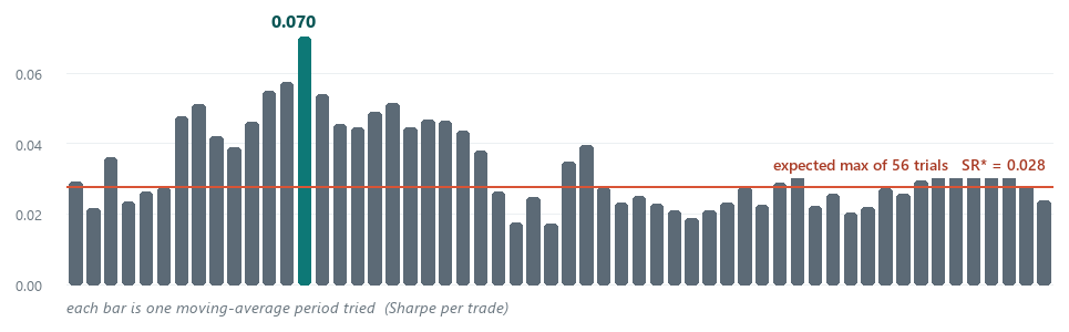
Each bar is one moving-average period that was tried. The horizontal line is the hurdle, 0.028: the Sharpe ratio expected from the best of 56 trials with no edge and the same spread. It is measured from 0 and not from the average of the bars, which is 0.034, so 31 of the 56 bars are above it. The winner at period 18 is about 1.3 standard errors of its own Sharpe ratio above the line.
The script prints this in the Experts tab. Lines 8 to 11 belong to the two controls of the next section.
Window: 6000 H1 bars of XAUUSD from 2025.08.12 10:00 to 2026.08.18 08:00, server LiteFinance-MT5-Demo.
Trials: 56 moving-average periods. Sample variance of their Sharpe ratios (varSR): 0.000144.
Best variant: period 18, 711 trades, per-trade Sharpe ratio 0.0704 (skewness 4.24, Pearson kurtosis 33.59).
PSR against 0 (sample length and shape of the returns): 98.5%.
Hurdle for 56 trials: 0.0279.
DSR (also accounts for the 56 trials): 90.6%.
Verdict: the best variant does not clear the 95% bar.
Control without an edge: 56 synthetic strategies, 600 trades each, seed 12345.
Best Sharpe ratio 0.1122, PSR 99.7%, hurdle 0.1013, DSR 60.5%: does not clear the 95% bar.
Control with a per-trade Sharpe ratio of 0.10: the same random draws plus the edge.
Best Sharpe ratio 0.2157, PSR 100.0%, hurdle 0.1015, DSR 99.7%: clears the 95% bar.
Wrote DeflatedSharpe_result.csv to the common Files folder.
The PSR accounts only for the 711 trades and for the shape of the returns: a skewness of 4.24 and a Pearson kurtosis of 33.6, which is 30.6 in excess terms. The result is 98.5 percent. In this sample the positive skewness outweighs the kurtosis. The expression under the square root, denom in the code, is 0.742, against 1.002 for normal returns. With normal returns, the same Sharpe ratio and trade count would give 96.9 percent. On its own, 98.5 percent looks like a significant result.
Then the deflation is applied. The hurdle for 56 trials is 0.028. Against that hurdle instead of 0, the same test gives a DSR of 90.6 percent. That is below the 95 percent bar that a result usually has to clear to be called significant. In standard errors, the winner is 1.3 above the hurdle, and 95 percent requires 1.645.
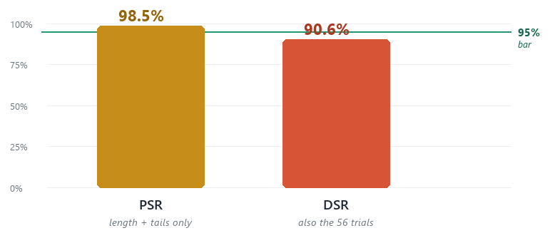
The same winning strategy, scored two ways. With the adjustment for sample length and the shape of the returns only, it clears the 95 percent bar. With the adjustment for the 56 variants as well, it does not. The gap between the two bars, about 8 percentage points, is what counting the search costs this result.
The result does not show that the strategy is bad, or that it is proven to be noise. It shows that the evidence does not clear the bar once the search is counted. A high Sharpe ratio read off the best of many runs is not, on its own, evidence of skill. The DSR takes the number of trials into account, and it is the figure to report after an optimization.
These figures come from one specific run: XAUUSD H1 on the LiteFinance-MT5-Demo server, with a window of 6,000 bars whose last bar opens at 2026.08.18 08:00 server time. The last bar of the window is left out of the calculation, because in a live run it is still forming. The values depend on the broker's price history, its server time zone, the symbol, the timeframe and the depth of the history. If any of them changes, the numbers change. To repeat this exact run, set InpEndTime to 2026.08.18 08:00 on that server. With the default of 0 the script takes the latest bars, so a run today gives different values.
Within a narrow range the conclusion is less sensitive than the decimals. We repeated the calculation on 81 windows, moving the end of the window by up to 40 bars in either direction. The best period stayed at 18 in all of them. The number of trades moved between 705 and 723, the PSR between 98.0 and 98.9 percent, the hurdle between 0.027 and 0.032, and the DSR between 88.9 and 91.2 percent. These windows overlap almost entirely, so this checks the decimals and is not an independent test.
Two controls with a known answer
In the market example the true answer is unknown. A test that rejects everything carries no information, and neither does a test that accepts everything. Before relying on the DSR, we have to see it on cases where the answer is known.
So the demo runs the same search twice more, on synthetic strategies. Each synthetic strategy draws 600 returns from a normal distribution. In the first control the mean is 0, so no strategy has an edge. In the second control every return gets a small positive mean, so every strategy has a known per-trade Sharpe ratio of 0.10. Both controls start from the same seed, 12345, so they use the same random draws and differ only in that mean. Each control has 56 strategies, the same count as the market sweep.
//+------------------------------------------------------------------+
//| One standard-normal draw by the Box-Muller transform             |
//+------------------------------------------------------------------+
double Gauss(void)
  {
   double u1 = (MathRand() + 1.0) / 32769.0;
   double u2 = (MathRand() + 1.0) / 32769.0;
   return(MathSqrt(-2.0 * MathLog(u1)) * MathCos(2.0 * M_PI * u2));
  }
//+------------------------------------------------------------------+
//| A synthetic strategy with a known per-trade Sharpe ratio: n      |
//| normal returns whose mean is edgeSharpe standard deviations.     |
//| With edgeSharpe = 0 the strategy has no edge.                    |
//+------------------------------------------------------------------+
void RunSynthetic(const double edgeSharpe, const int n, double &ret[])
  {
   double sigma = 0.01;
   double mu    = edgeSharpe * sigma;
   ArrayResize(ret, n);
   for(int i = 0; i < n; i++)
      ret[i] = mu + sigma * Gauss();
  }
The best strategy of each control is scored with PSR and DSR, the same two functions that score the market winner. The hurdle of a control comes from the variance of its own 56 Sharpe ratios, not from the market sweep.
//+------------------------------------------------------------------+
//| Control: the same search over nTrials synthetic strategies with  |
//| a known edge. Returns the DSR of the best one. varSR is the      |
//| sample variance of the Sharpe ratios of this set. The seed is    |
//| set again on every call, so two calls use the same random draws. |
//+------------------------------------------------------------------+
double RunControl(const double edgeSharpe, const int nTrials, double &bestSR, double &psr, double &srStar)
  {
   MathSrand(InpSeed);
   double sharpe[];             // Sharpe ratio of every synthetic strategy
   double best[];               // returns of the best one
   ArrayResize(sharpe, nTrials);
   bestSR = -1.0e10;
   for(int t = 0; t < nTrials; t++)
     {
      double r[];
      RunSynthetic(edgeSharpe, InpCtrlObs, r);
      sharpe[t] = CDeflatedSharpe::Sharpe(r);
      if(sharpe[t] > bestSR)
        {
         bestSR = sharpe[t];
         ArrayResize(best, ArraySize(r));
         ArrayCopy(best, r);
        }
     }
   double varSR = VarianceOf(sharpe);
   psr    = CDeflatedSharpe::PSR(best, 0.0);
   srStar = CDeflatedSharpe::ExpectedMaxSharpe(varSR, nTrials);
   return(CDeflatedSharpe::DSR(best, varSR, nTrials));
  }
Without an edge, the best of the 56 strategies shows a Sharpe ratio of 0.112 and a PSR of 99.7 percent. That PSR looks like a significant result, although no strategy in this set has an edge. The hurdle for this set is 0.1013, and the DSR is 60.5 percent. This is a false positive with a known answer, and the DSR does not pass it.
With the edge of 0.10, the best strategy reaches a Sharpe ratio of 0.216. That is about twice the edge it was built with, which is the selection effect again. Its PSR rounds to 100.0 percent. The hurdle for this set is 0.1015, almost the same as in the first control, and the DSR is 99.7 percent, above the 95 percent bar. With this edge in all 56 strategies and 600 trades each, the adjustment did not hide it.
The hurdle of the second control is about the same as the edge the strategies were built with. Read as a plain PSR, the DSR would say that the true Sharpe ratio is above 0.1015, and here it is 0.10. The DSR of a selected winner is not read that way. The hurdle is a rejection threshold under the hypothesis of no edge. It estimates how much the selection adds to the best observed Sharpe ratio when no strategy has an edge. Here 0.2157 minus 0.1015 leaves 0.1142, which is close to the edge of 0.10 and 2.8 standard errors above 0.
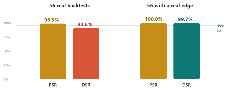
The same test on three cases. On 56 market backtests the winner does not clear the bar once the search is counted. On 56 synthetic strategies without an edge the PSR of the best one is 99.7 percent and its DSR is 60.5 percent. On the same 56 strategies with an edge of 0.10 the DSR is 99.7 percent.
The controls do not read the price history. With the default seed and 56 trials, their figures do not depend on the broker or the symbol.
The controls differ from the market example in more than the edge. The synthetic returns are normal and independent, with 600 trades per strategy. The market variants share one price history and have between 357 and 1,619 trades, and the returns of the winner are fat-tailed. In the second control all 56 strategies share the edge, which is a favorable case for the test. A search in which only one variant has an edge is a harder case, and the article does not test it. The controls show that the test separates these two synthetic cases. They are one seed and one edge size, not a study of how often the test is right.
Files and how to run it
The article has two attached files.
| File | What it holds |
|---|---|
| DeflatedSharpe.mqh | The CDeflatedSharpe class: the sample moments, the normal CDF and its inverse, the Sharpe ratio, the PSR, the hurdle and the DSR. All methods are static and the file has no includes. |
| DeflatedSharpeDemo.mq5 | A script that sweeps a moving-average strategy over a range of lookback periods, keeps the variant with the best Sharpe ratio, and prints its PSR and DSR. It then runs the same search on synthetic strategies without an edge and with a known edge. It writes DeflatedSharpe_result.csv with every variant and the results, and it does not trade. |
To reproduce it:
- Put DeflatedSharpe.mqh and DeflatedSharpeDemo.mq5 in the same folder under MQL5\Scripts and compile the script.
- Open a chart with enough history. A liquid symbol on an hourly timeframe works well. Attach the script to the chart and keep the defaults, or change the period range. With InpEndTime at 0 the window ends at the latest bar. Set a date and time to fix the window and repeat a run.
- Read the results in the Experts tab: the window, the trials and varSR, the best variant, the PSR, the hurdle, the DSR and the two controls. The file DeflatedSharpe_result.csv is in the common Files folder.
To evaluate your own strategy, you need per-trade returns in a double array. In the Strategy Tester you can build that array in OnTester. Load the closed deals with HistorySelect and read each realized profit with HistoryDealGetDouble and DEAL_PROFIT. Then divide that profit by the money at risk on the trade, or by the account equity at the time. DEAL_PROFIT is an amount of money, not a return, and with a changing position size it distorts the Sharpe ratio.
For a single strategy, pass the array to PSR. For an optimization, compute the per-trade Sharpe ratio of every pass with CDeflatedSharpe::Sharpe and take the sample variance of those values. Then pass the returns of the best pass, that variance and the number of passes to DSR. Each pass runs separately, so the per-pass values have to be collected with frames, or exported and processed afterwards. Do not use the Sharpe Ratio value of the tester report for this. It is not computed from per-trade returns, so it is in different units.
Limitations
- The DSR assumes that the trials are independent and that their Sharpe ratios are roughly normal. Neighboring lookback periods on one price series are strongly correlated, so the 56 trials are not 56 independent draws. In this run the spread between variants, 0.012, is smaller than the 0.032 standard error of the winner's own Sharpe ratio, which is what variants that move together produce. Correlation acts on the hurdle in two ways. The number of independent trials is below 56, but the script still passes 56, which keeps the hurdle high. The spread that varSR measures is smaller than for independent trials, which lowers the hurdle. The article does not measure how far the second effect offsets the first, and the verdict depends on it. With the same varSR, the DSR of the winner is 90.6 percent for 56 independent trials, 94.9 percent for 8 and 95.2 percent for 7.
- The number of trials must be counted in full. If you tried 100 variants over a week and only remember the last 50, the deflation is too weak. Counting fewer trials than were run lowers the hurdle and raises the DSR.
- The moments are estimated from the sample, so on short histories the skewness and the kurtosis are themselves noisy. In this run every variant had between 357 and 1,619 trades. The script itself only skips variants with fewer than 10 trades.
- The DSR measures statistical significance. It does not measure profitability after costs or performance out of sample. A strategy can pass the DSR and still fail on slippage, a regime change or a walk-forward split. It is one necessary check among several, and the 95 percent bar it is read against is a common convention.
- The tests assume that the per-trade returns are independent. They do not adjust for autocorrelation between consecutive trades or for overlapping market conditions, which can make the confidence look firmer than it is. They also work in per-trade units. A per-trade Sharpe ratio is not a time-based or annualized one, and variants with very different trade frequencies are not directly comparable on a time basis.
- The expected-maximum benchmark assumes that the Sharpe ratios of the trials are normally distributed. A skewed or fat-tailed spread of those values would move the hurdle up or down, so it is an estimate. The formula is also an approximation. For 56 independent normal draws it gives 2.32 standard deviations, and the exact expected maximum is 2.29.
- The trial count should include every research decision, not only the one parameter swept here. The symbol, the timeframe, the entry and exit rule, the history window and any filters all add to the real number of trials. Leaving them out understates the search.
- The DSR that the class returns is a probability between 0 and 1. It is not an adjusted Sharpe ratio.
- The moving-average example is a plain illustration. It uses close-to-close per-trade returns with no spread, commission or slippage. For a strategy that reverses this often, costs would change the return distribution and the result.
- The market example is one run: one symbol, one timeframe, one broker's history and one 6,000-bar window, checked only against shifts of up to 40 bars. The controls are one seed, one edge size and 600 normal, independent returns per strategy. Neither is a study of how often the test is right.
- Not clearing the bar is not evidence that there is no edge. A real but smaller edge, or a shorter sample, can also fall below 95 percent. With the input InpEdge set to 0.05 and the same seed, the best synthetic strategy has a DSR of 93.7 percent and does not clear the bar. The article does not measure that power in general, and it does not test the market winner out of sample.
Conclusion
A Sharpe ratio from a backtest is a starting point. The PSR turns it into a confidence statement that takes into account how many trades there are and how their returns are distributed. The DSR adds the adjustment that applies once you optimize: the number of variants tried before keeping the best.
On XAUUSD H1 the winner scored 98.5 percent on its own and 90.6 percent once all 56 variants were counted, below the 95 percent bar. That says the evidence is not sufficient at that threshold. It does not say that the strategy is proven worthless. On synthetic strategies the same test did not pass the best of 56 strategies without an edge, and it passed the best of 56 strategies with an edge of 0.10.
To use the class in your own research, pass it your per-trade returns, the variance of the Sharpe ratios of your trials and the trial count. It reports whether the evidence for the edge still clears the bar once the search is counted.
A final note: this is an educational article about a measurement tool, not a trading strategy and not financial advice. The value is the native, dependency-free code and a way to read your own backtests that counts the search.
Warning: All rights to these materials are reserved by MetaQuotes Ltd. Copying or reprinting of these materials in whole or in part is prohibited.
This article was written by a user of the site and reflects their personal views. MetaQuotes Ltd is not responsible for the accuracy of the information presented, nor for any consequences resulting from the use of the solutions, strategies or recommendations described.

 Features of Custom Indicators Creation
 Swing Extremes and Pullbacks (Part 5): Filtering Weak Swings Using Candle Imbalance
 Features of Experts Advisors
 Neural Networks in Trading: Robust Trading Signals in Any Market Regime (Conclusion)

- Free trading apps
- Over 8,000 signals for copying
- Economic news for exploring financial markets
You agree to website policy and terms of use