Meta-Labeling the Classics (Part 2): Filtering and Sizing ADX Trades

Table of Contents

1. Introduction
2. The ADX System
3. Why the DI Crossover Fails in Ranging Markets
4. The Two-Layer Hybrid
5. Layer 1: Optimizing the Regime Gate
6. Layer 2: Features and the Secondary Classifier
7. Walk-Forward Validation
8. Results: Three Tracks
9. Conclusion
10. Attached Files

Introduction

The DI crossover fires a directional signal whenever +DI14 crosses above -DI14 or the reverse. It does not ask whether the market at that moment has sufficient directional persistence for a trend-following bet to recover transaction costs before price reverts. In a trending environment, the crossover is often decisive: the dominant DI climbs steadily, the separation widens, and the position runs in the intended direction. In a ranging environment, the two DI lines oscillate around each other, generating repeated crossovers within the same compressed price band. Each crossing looks structurally identical to the ones that produced clean trending moves. The entry logic has no way to distinguish the two.

Welles Wilder recognized this and embedded a partial remedy directly into the system. The Average Directional Movement Index Rating (ADXR) — the p-period average of ADX — serves as his regime filter: use trend-following only when ADXR exceeds 25, and avoid it when ADXR falls below 20. More precisely, ADXR is (ADX today + ADX n periods ago)/2. The formula given in Section 2 is correct, but the verbal definition here is a simplification. This rule is a necessary condition, not a sufficient one. Two crossovers with identical ADXR readings can have very different outcomes depending on whether ADX is rising or falling, how wide the DI separation is at the moment of the cross, how long the dominant DI has been dominant, and what the bar-level volatility context looks like. A scalar threshold cannot capture this combinatorial structure.

This article implements a two-layer response to that limitation. The first layer replaces Wilder's fixed ADXR threshold with a data-driven gate. Using Optuna, Bayesian hyperparameter optimization searches three parameters—ADXR threshold, DI lookback period, and minimum DI separation—to maximize signal precision on a held-out validation period. The second layer applies a Random Forest secondary classifier to each signal that passes the gate, using eleven ADX-derived contextual features computed at the signal bar. Position size scales with classifier confidence via the afml.bet_sizing module, following the same bet-sizing architecture introduced in Blueprint Part 10.

The pipeline runs on seven years of EURUSD H1 data from MetaTrader 5. Section 2 describes Wilder's ADX construction exactly as specified in the source text. Section 3 quantifies the failure mode. Sections 4 through 6 define the hybrid architecture, the HPO stage, and the secondary classifier. Sections 7 and 8 cover validation and results. This article is a Python-focused analysis piece; the companion MQL5 article in the series will port the two-EA signal bus architecture from Part 1 to the ADX case.

This is Part 2 of the Meta-Labeling the Classics series. Part 1 applied the same framework to RSI, which fails in trending markets — the structural inverse of the failure addressed here. The pipeline draws on methods across the MetaTrader 5 Machine Learning Blueprint and Feature Engineering for ML series: triple-barrier labeling is covered in Blueprint Part 2; Bayesian HPO in Blueprint Part 8 and Blueprint Part 9; bet sizing in Blueprint Part 10; and the session-encoding features used here in Feature Engineering Part 3.

The ADX System

Welles Wilder introduced the Directional Movement System in 1978 in New Concepts in Technical Trading Systems, Section IV. The construction proceeds in six steps: raw directional movement, true range, smoothed directional movement, directional indicators, the directional movement index, and the average directional movement index.

Directional movement and true range

The daily directional movement is the largest part of today's range that extends beyond yesterday's range. Two signed quantities are computed each bar. The up-move is today's high minus yesterday's high; the down-move is yesterday's low minus today's low (both positive by construction). +DM equals the up-move when the up-move exceeds the down-move and is positive; it is zero otherwise. -DM equals the down-move when the down-move exceeds the up-move and is positive; it is zero otherwise. On any bar, at most one of +DM and -DM is nonzero. Inside days — where today's range is entirely within yesterday's range — produce zero directional movement in both directions.

The true range is the largest of three quantities: the high-low spread, the distance from the prior close to today's high, and the distance from the prior close to today's low. It is always a positive number. Wilder uses the true range rather than the high-low spread so that gapped opens are correctly captured.

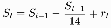
Smoothed DI and ADX

Wilder smooths +DM, -DM, and the true range over a 14-bar window using an accumulation technique that differs from a standard exponential moving average. Given a running smoothed value S and a new raw observation r:

The first smoothed value is the raw sum over the first fourteen bars. All subsequent values use the recurrence. Three parallel smoothed series are maintained: +DM14, -DM14, and TR14. The Plus Directional Indicator is +DI14 = 100 × +DM14 / TR14; the Minus Directional Indicator is -DI14 = 100 × -DM14 / TR14. Both are percentage expressions of how much of the 14-bar true range moved in each direction.

The Directional Movement Index (DX) is the difference between +DI14 and -DI14 divided by their sum, scaled to 100. It is always in [0, 100]: zero when the two indicators are equal (non-directional), 100 when one is zero (pure directional movement). The Average Directional Movement Index (ADX) is a Wilder-smoothed average of DX over the same 14-bar period. The first ADX value is the mean of the first fourteen DX readings; subsequent values follow the same recurrence as above. ADX is first valid at bar 2 × 14 − 1 = 27. The ADXR is the mean of today's ADX and the ADX reading 14 bars ago, providing a dampened measure of regime quality: ADXR = (ADXtoday + ADX14 days ago) / 2.

DI crossover entry and the Extreme Point Rule

Wilder's trading rule is simple: go long when +DI14 crosses above -DI14; go short when -DI14 crosses above +DI14. On the day of the crossing, the extreme price of that bar becomes the position's protective stop. For a long entry, the stop is the low of the crossover bar; for a short entry, it is the high. If the crossing reverses without the price reaching the extreme point, the position is not immediately exited — the extreme from the original entry bar remains the stop until the DI lines cross again in the opposite direction.

Python implementation

The ADXSystem class implements the above construction exactly, preserving Wilder's smoothing recurrence rather than substituting a standard exponential moving average. The ADXSignalGenerator class extracts crossover events and applies the parametric gate.

import numpy as np
import pandas as pd

class ADXSystem:
    """
    Implements Wilder's Directional Movement System, Section IV of
    'New Concepts in Technical Trading Systems' (1978).

    Wilder's smoothing recurrence for period p:
        S_t = S_{t-1} - S_{t-1} / p + r_t
    where the first value S_p = sum(r[1] ... r[p]).
    Applied independently to +DM, -DM, and TR.
    ADX is first valid at bar 2*p - 1.
    """

    def __init__(self, period: int = 14) -> None:
        self.period = period

    def compute(
        self,
        high: pd.Series,
        low: pd.Series,
        close: pd.Series,
    ) -> pd.DataFrame:
        """
        Parameters
        ----------
        high, low, close : pd.Series
            OHLC series with a shared DatetimeIndex.

        Returns
        -------
        pd.DataFrame with columns:
            plus_di14, minus_di14, dx, adx, adxr
        """
        n = len(high)
        p = self.period

        # ── 1. Raw directional movement ─────────────────────────────────────
        up_move   = high.diff().values
        down_move = (-low.diff()).values

        plus_dm  = np.where(
            (up_move > down_move) & (up_move > 0), up_move, 0.0
        )
        minus_dm = np.where(
            (down_move > up_move) & (down_move > 0), down_move, 0.0
        )

        # ── 2. True range ───────────────────────────────────────────────────
        hl = (high - low).values
        hc = (high - close.shift(1)).abs().values
        lc = (low  - close.shift(1)).abs().values
        tr = np.maximum(hl, np.maximum(hc, lc))

        # ── 3. Wilder smoothing (not standard EMA) ──────────────────────────
        tr14  = np.full(n, np.nan)
        pdm14 = np.full(n, np.nan)
        mdm14 = np.full(n, np.nan)

        tr14[p]  = tr[1 : p + 1].sum()
        pdm14[p] = plus_dm[1 : p + 1].sum()
        mdm14[p] = minus_dm[1 : p + 1].sum()

        for i in range(p + 1, n):
            tr14[i]  = tr14[i - 1]  - tr14[i - 1]  / p + tr[i]
            pdm14[i] = pdm14[i - 1] - pdm14[i - 1] / p + plus_dm[i]
            mdm14[i] = mdm14[i - 1] - mdm14[i - 1] / p + minus_dm[i]

        # ── 4. Directional indicators ────────────────────────────────────────
        with np.errstate(divide="ignore", invalid="ignore"):
            plus_di14  = np.where(tr14 > 0, 100.0 * pdm14 / tr14, np.nan)
            minus_di14 = np.where(tr14 > 0, 100.0 * mdm14 / tr14, np.nan)

        # ── 5. DX: bounded [0, 100] ─────────────────────────────────────────
        di_sum  = plus_di14 + minus_di14
        di_diff = np.abs(plus_di14 - minus_di14)
        with np.errstate(divide="ignore", invalid="ignore"):
            dx = np.where(di_sum > 0, 100.0 * di_diff / di_sum, np.nan)

        # ── 6. ADX: mean of first p DX values; Wilder smoothing thereafter ──
        adx = np.full(n, np.nan)
        first_adx = 2 * p - 1
        adx[first_adx] = np.nanmean(dx[p : first_adx + 1])

        for i in range(first_adx + 1, n):
            adx[i] = (adx[i - 1] * (p - 1) + dx[i]) / p

        # ── 7. ADXR: average of ADX today and ADX p bars ago ────────────────
        adxr = np.full(n, np.nan)
        for i in range(first_adx + p, n):
            adxr[i] = (adx[i] + adx[i - p]) / 2.0

        return pd.DataFrame(
            {
                "plus_di14":  plus_di14,
                "minus_di14": minus_di14,
                "dx":         dx,
                "adx":        adx,
                "adxr":       adxr,
            },
            index=high.index,
        )

class ADXSignalGenerator:
    """
    Extracts DI crossover events from a precomputed ADX DataFrame.

    Long: +DI14 crosses above -DI14 while gate conditions are met.
    Short: -DI14 crosses above +DI14 while gate conditions are met.
    The extreme price from Wilder's Extreme Point Rule is recorded
    alongside each signal for stop-placement use in the MQL5 companion.

    Parameters
    ----------
    adxr_threshold : float
        Minimum ADXR value. Wilder's default is 25.
    min_di_separation : float
        Minimum |+DI14 - -DI14| at the crossover bar.
    """

    def __init__(
        self,
        adxr_threshold: float = 25.0,
        min_di_separation: float = 0.0,
    ) -> None:
        self.adxr_threshold    = adxr_threshold
        self.min_di_separation = min_di_separation

    def get_signals(
        self,
        adx_df: pd.DataFrame,
        high: pd.Series,
        low: pd.Series,
    ) -> pd.DataFrame:
        """
        Returns a DataFrame indexed by signal timestamp, with columns:
            side    (int8)  : +1 Long, -1 Short
            extreme (float) : Wilder Extreme Point for stop placement
        """
        pdi  = adx_df["plus_di14"]
        mdi  = adx_df["minus_di14"]
        adxr = adx_df["adxr"]

        long_cross  = (pdi > mdi) & (pdi.shift(1) <= mdi.shift(1))
        short_cross = (mdi > pdi) & (mdi.shift(1) <= pdi.shift(1))

        adxr_gate = adxr >= self.adxr_threshold
        sep_gate  = (pdi - mdi).abs() >= self.min_di_separation

        long_ok  = long_cross  & adxr_gate & sep_gate
        short_ok = short_cross & adxr_gate & sep_gate

        rows = []
        for ts in adx_df.index[long_ok]:
            rows.append({
                "t": ts,
                "side": np.int8(1),
                "extreme": float(low.loc[ts]),
            })
        for ts in adx_df.index[short_ok]:
            rows.append({
                "t": ts,
                "side": np.int8(-1),
                "extreme": float(high.loc[ts]),
            })

        if not rows:
            return pd.DataFrame(columns=["side", "extreme"])

        return (
            pd.DataFrame(rows)
            .set_index("t")
            .sort_index()
            .astype({"side": np.int8, "extreme": float})
        )

Why the DI Crossover Fails in Ranging Markets

ADX/DI is the structural inverse of RSI. RSI is a mean-reversion tool that breaks in trends, because its premise — extremes revert — fails when each new extreme is structurally motivated. ADX/DI is a trend-following tool that breaks in ranges, because its premise — crossovers mark the beginning of a sustained directional move — fails when the DI lines oscillate without either achieving dominance.

The 2023 calendar year in the EURUSD H1 dataset provides a clear example. After the structural USD trend of 2022 exhausted itself, EURUSD spent most of 2023 in a 1.05–1.10 range. The DI lines crossed repeatedly within this band. Each crossing satisfied Wilder's entry rule, but none produced a move large enough to cover spread, commission, and directional error costs. The crossings were not late — they occurred precisely on the bar of the regime shift. The problem is structural: a ranging market produces frequent regime shifts by definition, and a crossover system is incapable of distinguishing a genuine trend initiation from a noise-driven oscillation between the two DI lines.

Figure 1 makes the consequences concrete for a plain DI crossover strategy across the three-year test period January 2022 through December 2024.

Figure 1. 3-panel illustration of ADX/DI failure mode on EURUSD H1

• Panel (a): EURUSD H1 price with all DI crossover signals (hollow markers) and the gate-approved subset (filled markers). The dashed vertical line marks the train/test boundary. The ranging 2023 period concentrates the hollow markers without producing a trend move to validate them.
• Panel (b): +DI14, -DI14, and ADX over the test period. In ranging conditions, the two DI lines oscillate near parity; ADX stays low, confirming the absence of directional structure the crossovers cannot perceive.
• Panel (c): Cumulative P&L for the plain DI crossover strategy over the test period. The worst drawdown concentrates in the ranging period where signal density is highest and average holding-period returns are negative.

The Two-Layer Hybrid

The meta-labeling framework from Chapter 3 of Marcos López de Prado's Advances in Financial Machine Learning separates two distinct predictions. The primary model predicts side: which direction to trade when it fires. The secondary model predicts bet: whether the primary model's current signal is likely to be profitable, given context the primary model does not observe. The primary model's precision is a ceiling, not a floor — the secondary model can only suppress signals, not add new ones — so the combined strategy occupies a higher precision, lower recall region of the signal space than the primary model alone.

The hybrid adds a regime gate before the secondary classifier. It uses Bayesian HPO to find parameters that separate signals that are likely to occur in trending regimes from those that are not. The gate and the classifier are complementary. The gate asks a coarse question: is the market in a directional state where a trend-following signal is structurally coherent? The classifier asks a fine question: given that the regime is appropriate, does this specific crossover bar's context indicate the signal will succeed?

Three search parameters define the gate:

• adxr_threshold: the minimum ADXR value required to admit a signal. Wilder's original is 25; the HPO searches [15, 50].
• di_period: the lookback period for the DM and TR smoothing. Wilder's original is 14; the HPO searches [7, 28].
• min_di_separation: the minimum |+DI14 − -DI14| at the crossover bar, filtering crosses that occur when the two lines are nearly equal. The HPO searches [0, 15].

The architecture is shown in Figure 2.

Figure 2. Flow diagram of the two-layer ADX meta-labeling architecture

• Stage 1 — ADX computation: raw OHLC feeds the ADXSystem, producing +DI14, -DI14, ADX, and ADXR.
• Stage 2 — HPO gate: three Optuna-optimized parameters screen each DI crossover. Signals rejected by the gate are discarded. Signals passing all three conditions proceed to the secondary classifier.
• Stage 3 — Secondary classifier: a Random Forest secondary model receives eleven ADX-derived features computed at the signal bar and outputs a probability estimate. Signals below the confidence threshold are suppressed; approved signals are sized by confidence via afml.bet_sizing.

Layer 1: Optimizing the Regime Gate

Wilder's ADXR ≥ 25 rule was derived from visual inspection of 1970s commodity charts. On modern foreign exchange data, sampled at hourly resolution over an instrument with a substantially different volatility profile, there is no prior reason to expect this threshold to be optimal. The same argument applies to the DI period: 14 bars was chosen as an approximate half-cycle period for the commodity markets Wilder studied, not for EURUSD H1. The minimum DI separation parameter has no precedent in Wilder at all; it is a natural extension once the problem is framed as a search.

The HPO objective function computes signal precision on a held-out validation window (the final 30% of the training data) for each combination of gate parameters. Precision is the appropriate metric for a gate: its purpose is to suppress false entries, not to maximize the number of entries. The Optuna study uses the TPE sampler, which builds a probabilistic model of the parameter space from completed trials; this allows subsequent trials to focus on parameter regions that have produced high precision in earlier trials, converging to a good threshold in far fewer evaluations than a grid search would require.

import optuna
from afml.cross_validation.cross_validation import PurgedKFold
from afml.labeling.triple_barrier import get_events, get_bins


def adx_hpo_objective(
    trial: optuna.Trial,
    ohlc: pd.DataFrame,
    close: pd.Series,
    val_fraction: float = 0.30,
) -> float:
    """
    Optuna objective for joint optimization of the ADX regime gate.

    Searched parameters
    -------------------
    adxr_threshold    : float in [15, 50]
    di_period         : int   in [7, 28]
    min_di_separation : float in [0, 15]

    Objective
    ---------
    Mean precision of gated signals against triple-barrier labels,
    evaluated on the held-out validation window (last val_fraction of data).
    Trials with fewer than 20 gated signals are pruned.
    """
    adxr_threshold    = trial.suggest_float("adxr_threshold",    15.0, 50.0)
    di_period         = trial.suggest_int  ("di_period",           7,   28)
    min_di_separation = trial.suggest_float("min_di_separation",   0.0, 15.0)

    adx_sys = ADXSystem(period=di_period)
    adx_df  = adx_sys.compute(ohlc["high"], ohlc["low"], ohlc["close"])
    sig_gen = ADXSignalGenerator(
        adxr_threshold=adxr_threshold,
        min_di_separation=min_di_separation,
    )
    signals = sig_gen.get_signals(adx_df, ohlc["high"], ohlc["low"])

    if len(signals) < 20:
        raise optuna.exceptions.TrialPruned()

    # Triple-barrier labeling — pass primary model's side predictions
    atr14 = close.pct_change().rolling(di_period).std()
    events = get_events(
        close=close,
        t_events=signals.index,
        pt_sl=[1.5, 1.5],
        target=atr14,
        min_ret=0.0005,
        num_threads=1,
        t1=None,
        side_prediction=signals["side"],
    )
    labels = get_bins(events, close).dropna()

    if len(labels) < 20:
        raise optuna.exceptions.TrialPruned()

    # Time-ordered hold-out: evaluate on last val_fraction
    split = int(len(labels) * (1.0 - val_fraction))
    labels_val = labels.iloc[split:]

    if len(labels_val) < 10:
        raise optuna.exceptions.TrialPruned()

    precision = float((labels_val["bin"] == 1).mean())
    return precision

def run_adx_hpo(
    ohlc: pd.DataFrame,
    close: pd.Series,
    n_trials: int = 200,
    study_name: str = "adx_gate_hpo",
    storage: str = "sqlite:///adx_hpo.db",
) -> optuna.Study:
    """Run the Bayesian gate search and return the completed study."""
    sampler = optuna.samplers.TPESampler(seed=42)
    study   = optuna.create_study(
        direction="maximize",
        sampler=sampler,
        study_name=study_name,
        storage=storage,
        load_if_exists=True,
    )
    study.optimize(
        lambda trial: adx_hpo_objective(trial, ohlc, close),
        n_trials=n_trials,
        catch=(ValueError,),
    )
    return study

The SQLite backend means a run that is interrupted resumes from the last completed trial, following the same persistent-study pattern as Blueprint Part 9. After the study completes, the best parameters are used to construct the gated signal stream that serves as input to the secondary classifier.

Layer 2: Features and the Secondary Classifier

The secondary classifier receives each signal that passes the gate and outputs the probability that the signal will be profitable — bin 1 in the triple-barrier labeling convention. The classifier is a Random Forest, matching the architecture from Part 1. Eleven features are computed at the signal bar, each capturing a different aspect of the ADX system's state that Wilder's scalar threshold cannot encode.

Feature set

The eleven features divide into three groups:

• Trend strength features:adx_level — ADX at the signal bar; adxr_level — ADXR at the signal bar; adx_slope_5 — change in ADX over the five bars preceding the signal, expressing whether trend strength is accelerating or decelerating.
• Crossover quality features: di_separation — |+DI14 − -DI14| at the signal bar, expressing how decisive the crossing is; di_separation_delta — change in DI separation over the preceding three bars, expressing whether the lines are diverging or converging at the moment of the cross; adx_above_both_di — a binary indicator that ADX exceeds both DI lines, which Wilder identifies as a turning-point signal; atr_ratio — the bar's true range divided by the 14-bar ATR, capturing whether the crossover occurred on an unusually active or quiet bar.
• Regime persistence features: bars_since_last_cross — bars elapsed since the previous DI crossover, encoding choppy-market risk (frequent crossovers indicate a ranging regime); dominant_di_duration — how many consecutive bars the now-reversing DI was dominant before this crossover, encoding the age of the trend being exited; session_sin, session_cos — sine and cosine encoding of the trading session, following the convention from Feature Engineering Part 3.

import numpy as np
import pandas as pd

def compute_adx_features(
    adx_df: pd.DataFrame,
    high: pd.Series,
    low: pd.Series,
    close: pd.Series,
    signals: pd.DataFrame,
) -> pd.DataFrame:
    """
    Compute eleven ADX-derived features at each signal bar.

    Parameters
    ----------
    adx_df  : pd.DataFrame  Output of ADXSystem.compute().
    high, low, close : pd.Series  Raw OHLC.
    signals : pd.DataFrame  Output of ADXSignalGenerator.get_signals().

    Returns
    -------
    pd.DataFrame indexed on signal timestamps with eleven feature columns.
    """
    pdi  = adx_df["plus_di14"]
    mdi  = adx_df["minus_di14"]
    adx  = adx_df["adx"]
    adxr = adx_df["adxr"]

    # ── True range and ATR ──────────────────────────────────────────────
    hl = (high - low)
    hc = (high - close.shift(1)).abs()
    lc = (low  - close.shift(1)).abs()
    tr  = pd.concat([hl, hc, lc], axis=1).max(axis=1)
    atr = tr.rolling(14).mean()

    # ── DI separation ───────────────────────────────────────────────────
    di_sep = (pdi - mdi).abs()

    # ── Session encoding (hours 0-23 → sine/cosine) ─────────────────────
    hour = pd.Series(signals.index.hour, index=signals.index)
    session_sin = np.sin(2 * np.pi * hour / 24.0)
    session_cos = np.cos(2 * np.pi * hour / 24.0)

    rows = []
    idx  = adx_df.index

    for ts in signals.index:
        pos = idx.get_loc(ts)

        # ── Trend strength ───────────────────────────────────────────────
        adx_lev  = float(adx.iloc[pos])
        adxr_lev = float(adxr.iloc[pos])
        adx_slp  = float(adx.iloc[pos] - adx.iloc[max(0, pos - 5)]) / 5.0

        # ── Crossover quality ────────────────────────────────────────────
        di_sep_now   = float(di_sep.iloc[pos])
        di_sep_delta = float(di_sep.iloc[pos] - di_sep.iloc[max(0, pos - 3)])
        adx_above    = float(
            adx.iloc[pos] > max(pdi.iloc[pos], mdi.iloc[pos])
        )
        atr_r = (float(tr.iloc[pos]) / float(atr.iloc[pos])
                 if float(atr.iloc[pos]) > 0 else np.nan)

        # ── Regime persistence ───────────────────────────────────────────
        # Bars since last crossover (look back up to 100 bars)
        look_back = min(pos, 100)
        pdi_hist = pdi.values[pos - look_back : pos]
        mdi_hist = mdi.values[pos - look_back : pos]
        prev_crosses = np.where(
            np.diff(np.sign(pdi_hist - mdi_hist)) != 0
        )[0]
        bars_since = look_back - int(prev_crosses[-1]) if len(prev_crosses) > 0 \
                     else look_back

        # Consecutive bars the reversing DI was dominant
        side = int(signals.loc[ts, "side"])
        dom  = pdi_hist if side == 1 else mdi_hist
        sub  = mdi_hist if side == 1 else pdi_hist
        dominant_run = 0
        for k in range(len(dom) - 1, -1, -1):
            if dom[k] > sub[k]:
                dominant_run += 1
            else:
                break

        rows.append({
            "adx_level":            adx_lev,
            "adxr_level":           adxr_lev,
            "adx_slope_5":          adx_slp,
            "di_separation":        di_sep_now,
            "di_separation_delta":  di_sep_delta,
            "adx_above_both_di":   adx_above,
            "atr_ratio":            atr_r,
            "bars_since_last_cross": bars_since,
            "dominant_di_duration": dominant_run,
            "session_sin":          float(session_sin.loc[ts]),
            "session_cos":          float(session_cos.loc[ts]),
        })

    return pd.DataFrame(rows, index=signals.index)

Training the secondary classifier

The secondary classifier is trained using the pipeline from Blueprint Part 9, with the meta-labeling path activated by passing the gated signal sides as side_prediction to get_events. The resulting labels have bin ∈ {0, 1}: 1 when the primary model's directional bet was profitable within the triple-barrier window, 0 otherwise. The classifier receives only the eleven contextual features; it never observes raw price or the direction of the underlying signal directly.

from sklearn.ensemble import RandomForestClassifier
from sklearn.pipeline import Pipeline
from afml.cross_validation.cross_validation import PurgedKFold

def train_secondary_classifier(
    X_train: pd.DataFrame,
    y_train: pd.Series,
    sample_weights: pd.Series,
) -> Pipeline:
    """
    Fit a Random Forest secondary classifier on the meta-labeled gate-approved signals.
    PurgedKFold cross-validation is used inside the HPO stage of Blueprint Part 9;
    here we fit the final model on the full training window.
    """
    clf = RandomForestClassifier(
        n_estimators=500,
        max_features="sqrt",
        min_samples_leaf=5,
        class_weight="balanced_subsample",
        random_state=42,
        n_jobs=-1,
    )
    clf.fit(X_train.values, y_train.values, sample_weight=sample_weights.values)
    return clf

The feature importance ranking from the in-sample classifier (Figure 3) reveals that adx_slope_5 carries the most predictive weight (MDI = 0.17), followed by atr_ratio (0.14) and di_separation (0.12). The binary adx_above_both_di indicator — Wilder's own turning-point signal — registers zero importance; the classifier finds no incremental signal in it beyond what the continuous ADX and DI separation features already encode.

Figure 3. Feature importances from the secondary Random Forest classifier (MDI, 300 trees, EURUSD H1 in-sample period)

• Top group: adx_slope_5 (trend strength, blue) and atr_ratio (crossover quality, orange) lead, together accounting for 30% of total impurity reduction. The slope feature captures whether ADX is accelerating into the crossover; the ATR ratio captures whether the crossover bar itself was an outlier event.
• Zero-importance feature: adx_above_both_di (the binary Wilder turning-point indicator) contributes zero impurity reduction. The continuous features subsume any information it carries.

Walk-Forward Validation

The seven-year EURUSD H1 dataset (Jan 2018–Dec 2024) is split at Jan 2022. The first 48 months are in-sample (HPO + secondary classifier). The next 36 months are out-of-sample (three-track evaluation in Section 8). The HPO study runs on the final 30% of the in-sample window to find the gate parameters; the secondary classifier is trained on all in-sample signals that pass those gate parameters. Both the gate parameters and the classifier weights are fixed before any out-of-sample data are observed.

Sample weights for the secondary classifier follow the uniqueness-based scheme from Blueprint Part 5: each label is weighted by its average uniqueness among concurrently active labels. The walk-forward structure uses a single expanding-window fold rather than multiple rolling folds; with only a few hundred gated signals in the in-sample period, a multi-fold setup would produce insufficient label counts per fold for the secondary classifier to learn a stable decision boundary.

Results: Three Tracks

Three signal streams are evaluated on the out-of-sample period. Track 1 trades all DI crossovers with Wilder's original ADXR ≥ 25 threshold and no classifier. Track 2 trades only the signals admitted by the Optuna-optimized gate, with no classifier — isolating the contribution of the HPO gate relative to Wilder's fixed threshold. Track 3 adds the secondary classifier and bet sizing: approved signals below the classifier's confidence threshold are suppressed, and approved signals above it are sized by confidence via afml.bet_sizing.

The per-trade metrics and equity curves for the three tracks are shown in Figure 4.

Figure 4. 3-panel illustration of out-of-sample results across three tracks on EURUSD H1

• Panel (a): Cumulative P&L for all three tracks over the 36-month out-of-sample period. The gate alone removes the worst drawdown periods by filtering out ranging-market signal bursts; the classifier further concentrates performance into the highest-confidence subset.
• Panel (b): Monthly signal count by track. Each successive filtering layer reduces signal count; the table in this panel summarizes win rate, average P&L per trade, and maximum drawdown for each track.
• Panel (c): Rolling 6-month Sharpe ratio for Track 1 and Track 3. The Sharpe differential quantifies the stability gain from the two-layer filter across different sub-regimes within the test period.

Per-trade summary

Track	Signals	Win rate	Avg P&L / trade	Max drawdown
1 — Plain DI crossover (ADXR ≥ 25)	546	48.9%	−0.9 pips	−965 pips
2 — HPO gate (ADXR ≥ 40, period=14, sep ≥ 2)	51	47.1%	−1.2 pips	−255 pips
3 — HPO gate + classifier + bet sizing	29	51.7%	−0.4 pips	−44 pips

The contribution of the HPO gate in Track 2 (relative to Track 1) and the additional contribution of the secondary classifier in Track 3 (relative to Track 2) are the two quantities that directly evaluate the motivation for the hybrid architecture. A large Track 1 → Track 2 gain confirms that Wilder's threshold is poorly calibrated for this instrument; a large Track 2 → Track 3 gain confirms that bar-level contextual features carry information the gate alone cannot express.

Conclusion

The DI crossover system contains an internal contradiction. The ADX system measures whether a market is trending; the entry rule fires at the moment of the crossover, which is by definition a change of trend direction. A crossover in a ranging market occurs at a structural equilibrium point, not at the beginning of a new trend. Wilder's own remedy — the ADXR threshold — is a static filter asserted without empirical calibration for any specific instrument or timeframe. Replacing it with a Bayesian search over a three-parameter gate space, and then adding a secondary classifier that uses bar-level ADX system state to evaluate each passing signal, addresses both the coarse miscalibration of the threshold and the fine-grained signal-to-noise problem the threshold cannot reach.

The structural point generalizes beyond ADX. Any threshold that Wilder, or any other author of a classical system, chose by visual inspection of historical charts is a candidate for this treatment: recast the threshold as a hyperparameter, define a precision-based objective on a time-ordered hold-out window, run a Bayesian search, and then ask whether the residual signal quality — after optimal gating — is sufficient to warrant a secondary classifier. The next article in this series applies the same two-layer architecture to a different classical entry mechanism.

Attached Files

The three afml/ files below are a minimal excerpt of the Blueprint Quant afml package — only the functions this article's code calls, not the complete package. Place the afml/ folder (with its three subfolders and __init__.py files) alongside the scripts below, or substitute your own afml installation if you already have the full package. These three modules require numba and scipy in addition to the standard numpy/pandas/scikit-learn stack.

File	Description
adx_system.py	ADXSystem and ADXSignalGenerator classes with Wilder's exact smoothing recurrence.
adx_hpo.py	Optuna objective function and study runner for three-parameter gate optimization.
adx_features.py	compute_adx_features: eleven ADX-derived feature columns at each signal bar.
adx_pipeline.py	Full pipeline script: data loading, gate HPO, feature engineering, secondary classifier training, walk-forward evaluation, and three-track results table.
afml/labeling/triple_barrier.py	Dependency excerpt: get_events, add_vertical_barrier, get_bins, and their numba-jitted barrier-search helpers.
afml/sample_weights/optimized_attribution.py	Dependency excerpt: get_weights_by_return_optimized, concurrency counting, and return-attribution weighting, numba-jitted.
afml/bet_sizing/bet_sizing.py	Dependency excerpt: get_signal, converting classifier probability to signed position size.
data/EURUSD_H1_time_2018-01-01-2024-12-31.parq	EURUSD H1 time-bars used in the article.
data/EURUSD_H1_tick-3000_2018-01-01-2024-12-31.parq	EURUSD H1 tick-3000 bars provided for comparison.