Machine Learning Under Constraint (Part 2): Calibrating Position Size to the Remaining Drawdown Budget

Table of Contents

1. Introduction
2. Why a Sigmoid, Not a Threshold
3. The Calibration Chain (WParamCalibrator)
4. What the Chain Actually Outputs
5. Production Problem: A Constraint With No Consumer Anywhere
6. Opinion: Two More Hardcoded Numbers That Should Stay Hardcoded
7. Conclusion
8. Attached Files

Introduction

Part 1 of this series tackled the foundational problem of abstraction. It replaced FundedNext's rigid, hardcoded rule constants with an explicit PropFirmRuleSet and refactored PropFirmAccountState to compute the remaining risk budget (risk_budget_pct) dynamically. With that refactor in place, the system can correctly interpret the daily and overall loss limits for any loaded program—whether it follows the fixed 5% daily limit of FundedNext, the variable scaling of a dynamic drawdown program, or a custom proprietary structure. However, as noted in the conclusion of Part 1, computation without consumption is inert. The account state knows exactly how much leash remains, but the position sizing engine was still looking at the old, hardcoded rules.

This article bridges that gap by implementing the consumer of that knowledge: the WParamCalibrator. This calibrator takes the abstract risk_budget_pct and translates it into a concrete sigmoid w parameter. This w-parameter is then fed into PropFirmAwareSizer, which scales every new position continuously between full size and zero as the daily budget erodes. This architecture is deliberately modular: the calibrator does not care whether the underlying program uses a daily limit, an overall limit, or a trailing maximum drawdown. It only sees the consolidated remaining budget fraction. This separation of concerns means that when we introduce a new prop firm rule set in the future, the sizing logic remains untouched.

This installation covers the calibration chain in detail. It explains why a sigmoid is used instead of a hard threshold, derives the calibration math, and visualizes the output across the full daily budget range. The article also identifies a gap found during a deep-dive review: the sizer validates max_leverage but never enforces it. Rather than patching this oversight haphazardly, I scope where the fix properly belongs. Finally, the article includes a dedicated tuning guide for the safety_factor—a parameter that quants often misconstrue as a static constant when it is, in fact, highly strategy-dependent.

Why a Sigmoid, Not a Threshold

At first glance, the problem of position sizing under a loss limit appears to be a textbook case for a threshold function. The logic seems intuitive: while risk_budget_pct remains above a certain cutoff (say, 20% of the daily limit remaining), trade at full size. Once the budget drops below that cutoff, cease trading entirely. This binary approach is exceptionally simple to implement, easy to reason about, and trivial to explain in a risk memo to stakeholders. It is also deceptively dangerous in a path-dependent trading environment.

A threshold creates a discontinuity in the sizing function. Imagine a scenario where a strategy takes a series of five small losses, each consuming 4% of the daily budget. The account starts at 100%, moves to 96%, 92%, 88%, 84%, and finally 80%. If the threshold is set at 80%, the trader is trading full size through the first four losses and then, upon the fifth loss, the position size drops from full to zero instantaneously. There is no warning, no gradual tightening of risk, and no signal that the edge of the cliff is approaching until the strategy has already fallen off it. In an automated system, this sudden shift can trigger catastrophic whipsaw effects, especially if the strategy relies on momentum or mean-reversion that typically strengthens during drawdowns.

bet_size_sigmoid and get_w, as defined in AFML Snippet 10.4, were originally designed to solve a different but structurally identical problem: mapping a forecast-price divergence into a bounded position size. Part 11 of the MetaTrader 5 Machine Learning Blueprint series borrowed that machinery and repurposed its input. Instead of calibrating against price divergence, WParamCalibrator calibrates against the remaining risk budget. The sigmoid maps each incremental budget decrease to a smooth decrease in the maximum allowable position size. As the budget approaches zero, the gradient of the position size curve increases, effectively tightening the leash at an accelerating rate without ever introducing a vertical cliff. The threshold's hard edge becomes a continuous, monotonic decline, avoiding the bar-to-bar discontinuity that can plague threshold-based systems. The only exception occurs at true exhaustion—when the budget is mathematically zero—which Section 3 covers as an explicit branch rather than a limit of the formula.

The Calibration Chain (WParamCalibrator)

The calibration chain is a three-step transformation pipeline. Each step performs a distinct mathematical operation, and the output of one feeds directly into the next. Understanding this flow is critical for quants who wish to modify the system's behavior.

risk_budget_pct  --[stop_loss_pct, safety_factor]  -->  cal_bet_size
cal_bet_size     --[cal_divergence, get_w]         -->  w_param
w_param          --[bet_size_sigmoid]              -->  sigmoid_scale

def calibrate(self, state: PropFirmAccountState) -> float:
    """Compute the sigmoid w parameter from the current account state."""
    risk_budget_pct = state.risk_budget_pct

    # Maximum allowable bet size at full signal strength:
    #   position x stop_loss <= risk_budget x safety_factor
    cal_bet_size = (risk_budget_pct * self.safety_factor) / self.stop_loss_pct
    cal_bet_size = float(np.clip(cal_bet_size, 0.0, 0.98))

    if cal_bet_size < 0.02:
        return np.inf  # budget exhausted - sigmoid collapses to zero

    return get_w(
        price_div=self.cal_divergence,
        m_bet_size=cal_bet_size,
        func="sigmoid",
    )

The first step calculates cal_bet_size. This value answers a precise quantitative question:

given the fraction of the loss budget still available, and given a fixed per-trade stop-loss percentage (as a fraction of the account equity), what is the largest fractional bet size the account can afford if the signal is at full confidence?

The formula is a direct proportionality: cal_bet_size = (risk_budget_pct * safety_factor) / stop_loss_pct. The safety_factor (typically less than 1.0) acts as a buffer. It holds back a portion of the budget to absorb non-stop-loss costs such as commissions, swaps, and—critically—the gap risk that occurs when the market jumps over the stop-loss level during high volatility. If the safety factor were set to 1.0, the calibrator would allow the full budget to be placed at risk, leaving zero room for transaction costs. In practice, setting it this high is almost guaranteed to breach the daily limit due to execution friction.

Tuning the safety_factor for Your Strategy: This is not a global constant; it must be derived from the strategy's specific cost structure and the instrument's volatility profile. For a high-turnover intraday scalper who executes dozens of trades per day, cumulative commissions and bid-ask slippage can easily consume 10–15% of the daily loss budget. For such a strategy, a safety factor of 0.60 to 0.65 is appropriate. Conversely, a swing trader who holds positions for several days and trades only once or twice a week faces negligible commission drag but must contend with overnight gap risk—the factor should be set higher, closer to 0.80 or 0.85, to ensure that a gap beyond the stop does not wipe out the budget. A robust tuning method involves running a backtest over a sample of high-volatility periods, recording the actual slippage (the difference between the stop price and the fill price) and the total commission paid per trade. The safety factor should be calibrated so that the cumulative costs never exceed the buffer in the worst-case scenario. This transforms the factor from an arbitrary number into a data-driven safeguard.

Once cal_bet_size is determined, the second step inverts the sigmoid via get_w. This function finds the w parameter that forces bet_size_sigmoid to output exactly cal_bet_size at the reference divergence cal_divergence. The result is that a fully-confident signal (where stage1_signal equals cal_divergence) will land precisely on the ceiling that the budget allows. Any signal with lower confidence will produce a position size that scales proportionally below this ceiling. The inversion itself is computationally non-trivial—it typically involves a numerical root-finding routine (such as bisection or Newton-Raphson) because the sigmoid equation cannot be solved analytically for w in closed form. This computational cost is acceptable because the calibrator is invoked once per sizing decision, not on every price tick in between.

Two numbers in this function are deliberately hardcoded rather than drawn from PropFirmRuleSet: the 0.98 ceiling and the 0.02 exhaustion floor. Section 6 provides a detailed justification for why these belong in the calibration logic itself rather than in the configuration layer, but the short version is that they are arithmetic safety guards for the sigmoid transformation, not business rules prescribed by any prop firm.

What the Chain Actually Outputs

Running WParamCalibrator with its default parameters (stop_loss_pct=0.01, safety_factor=0.70, cal_divergence=0.90) across the complete domain of risk_budget_pct produces a curve whose shape is both surprising and instructive. Figure 1 visualizes this relationship in two panels.

The w-parameter calibration chain's output across a full budget range

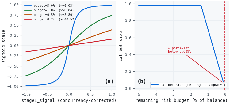
Figure 1. Two-panel illustration of the w-parameter calibration chain

• Left panel: bet_size_sigmoid as a function of stage1_signal at four distinct calibrated w values, each corresponding to a different budget level. At 5% of the balance remaining, w is extremely small (0.03), yielding a sigmoid that approximates a step function. This means the sizer reaches full size almost immediately as the signal crosses zero. At the opposite extreme, with only 0.2% of the budget remaining, w spikes to 40.5, and the sigmoid flattens dramatically. Even a perfect, fully-confident signal barely manages to reach a position size of 0.15.
• Right panel: The derived cal_bet_size ceiling—the maximum allowable position for a fully-confident signal—plotted directly against the remaining budget. The curve is perfectly flat at the 0.98 cap until the remaining budget drops below approximately 1.4% of the account balance. After this inflection point, the ceiling falls linearly toward the exhaustion floor.

The flat region in the right panel is the most important empirical finding of this analysis. It directly contradicts the intuition that de-risking should be a gradual, day-long process. With the default settings, solving the equation risk_budget_pct * 0.70 / 0.01 = 0.98 yields the threshold of 1.4%. In practical terms, on a $100,000 FundedNext account with a 5% daily loss limit ($5,000), the calibrator imposes essentially no constraint on position sizing until the account has already lost $3,600 of that $5,000 buffer — 72% of the daily limit consumed with the ceiling still sitting at 0.98. Only the last $1,400 (the remaining 28%) triggers the scaling mechanism. This means the great majority of the calibrator's dynamic range is compressed into the final fifth of the budget, not spread evenly across it.

This is a direct mechanical consequence of the default stop_loss_pct and safety_factor, not an inherent property of the sigmoid curve itself. If a trader employs a wider stop-loss (e.g., 2% instead of 1%), the flat region shrinks, and the de-risking begins earlier. Conversely, a narrower stop pushes the threshold even closer to zero. Before deployment, re-derive the threshold using your own stop_loss_pct. Do not assume the 1.4% figure applies to other configurations.

Cumulative Loss	risk_budget_pct	cal_bet_size	Position Ceiling
$0	0.0500	3.50 → 0.98 (capped)	Full size
$1,000	0.0400	2.80 → 0.98 (capped)	Full size
$2,000	0.0300	2.10 → 0.98 (capped)	Full size
$3,000	0.0200	1.40 → 0.98 (capped)	Full size
$3,600 (threshold)	0.0140	0.98	At ceiling — begins to decline
$4,000	0.0100	0.70	70% of full size
$4,500	0.0050	0.35	35% of full size
$4,900	0.0010	0.07	7% of full size

Table 1. cal_bet_size at representative cumulative-loss points, $100,000 account, 5% ($5,000) FundedNext daily limit, stop_loss_pct=0.01, safety_factor=0.70. Reproduced from the calibration formula in Section 3, not re-derived independently — Figure 1's right panel plots this same relationship continuously.

This raises an empirical question that static analysis cannot answer. Is concentrating calibration into the last 1.4% beneficial, or does it under-protect the account earlier and overreact at the end? The answer hinges entirely on the joint distribution between stage1_signal and risk_budget_pct. If losing streaks (which drive the budget down) tend to coincide with periods of high signal confidence—perhaps because the strategy's edge is strongest during trending markets, which also produce low-volatility losses—then the calibrator's aggressive full-sizing is justified.

Conversely, if losses tend to occur when the signal is already weak, the lack of early de-risking is a structural flaw. This is a question for backtesting, not algebra. A follow-up article in this series will present comprehensive backtest results across multiple prop-firm rule sets, examining whether the calibrated sigmoid reduces the probability of a daily-limit breach without prematurely cutting winning trades. For now, the calibration analysis confirms that the chain behaves as mathematically intended; the performance evaluation remains an open empirical question.

Production Problem: A Constraint With No Consumer Anywhere

This issue was not discovered by scanning the code in isolation; it surfaced from a direct, pragmatic question:

why does max_leverage never appear in any sizing calculation, despite being rigorously validated in PropFirmRuleSet.__post_init__ and being explicitly defined in rule sets such as FUNDEDNEXT_STELLAR_2STEP (where it is typically set to 100:1 for FX, 30:1 for commodities and 1:1 for crypto)?

On the surface, this looks like a simple oversight—a missing line of code. However, upon deeper inspection, it reveals a fundamental architectural gap in the pipeline.

Every quantity that WParamCalibrator and PropFirmAwareSizer compute is a fractional bet size in the range [-1, 1]. This is purely a risk-allocation signal, representing the percentage of the equity the strategy is willing to risk on a single trade. It is not a lot size, and it is not a notional exposure in dollars. max_leverage, on the other hand, constrains a completely different quantity: the margin-to-equity ratio. The relationship is defined as:

margin_required = notional / max_leverage, where the notional is the lot size multiplied by the instrument's price and contract size.

The current subpackage lacks the conversion logic that translates a fractional bet size into a lot size. That conversion happens downstream, in the execution layer—the backtester or the Expert Advisor—that turns final_size into an actual order volume (e.g., 1.5 lots). Because this translation layer does not exist within afml.prop_firm, there is no point in the pipeline where max_leverage could even be checked. The constraint is not checked in the wrong place; it has no place to be checked at all.

This is a distinctly different category of gap from the unused constants described in Part 1. Fields like min_trading_days and commission_per_lot were factual metadata sitting inert, waiting for a future consumer to use them. max_leverage, however, is a hard constraint that sits in the same logical category as daily_loss_limit_pct. Risk-based sizing does not automatically respect leverage caps. The two constraints are mathematically orthogonal: risk-based sizing controls the cost incurred if the stop-loss is hit, whereas leverage caps control the maximum notional exposure that can be opened in the first place, entirely independent of where the stop is placed. They only happen to align by coincidence, and that coincidence breaks down severely on instruments where the contract size is large relative to typical stop distances. Consider Gold (XAUUSD) at $2,500 per ounce with a standard 100 oz lot, making one lot worth $250,000 in notional. On a $100,000 account with max_leverage set to 30:1, the maximum allowable lots are calculated as:

max_lots = (account_equity × max_leverage) / (price × contract_size)

max_lots = (100,000 × 30) / (2,500 × 100) = 12.0 lots

If the risk-based sizing logic returns 15 lots (e.g., a high-confidence signal with a tight stop), the leverage cap would truncate this to 12 lots. Without this check, the EA would attempt to place an order for 15 lots, which the broker would likely reject. Worse, some brokers might accept it with an "over-leverage" warning, exposing the trader to a margin call and a violation of the prop firm's terms. The issue is even more pronounced on smaller accounts. A $25,000 account would have a maximum of 3 lots, which is drastically lower than what the risk-based sizing might suggest. The fix requires a dedicated function:

leverage_cap_lots(account_equity, price, contract_size, max_leverage)

applied at the precise point where final_size is translated into an order volume:

lots = min(risk_based_lots, leverage_cap_lots(...))

That translation layer, which converts fractional size to lots, does not currently exist in afml.prop_firm. Consequently, the fix does not belong in sizing.py as a quick patch; it belongs as the foundational piece of whatever module eventually owns the order execution interface. Implementing it as a patch would be an architectural violation, coupling the risk logic with execution details. This is out of scope for this article and is a strong candidate for a later installment in this series.

Opinion: Two More Hardcoded Numbers That Should Stay Hardcoded

Part 1's Opinion section argued that the 80%/30% thresholds inside derisking_factor belong outside PropFirmRuleSet because they represent a discretionary strategy choice rather than a factual rule of the prop firm. That argument set a precedent for delineating "business logic" from "arithmetic safety." WParamCalibrator.calibrate introduces two numbers that test this principle: the 0.98 ceiling and the 0.02 exhaustion floor. I argue that these should remain hardcoded for the same reasons.

Neither 0.98 nor 0.02 describes any aspect of FundedNext's terms of service, nor does it describe any other prop firm's rule set. You will not find a clause in any contract requiring the sigmoid to cap at 98% or floor at 2%. 0.98 is a pragmatic engineering margin against a mathematical artifact: the sigmoid function's range approaches 1.0 asymptotically but never actually reaches it at a finite w. Requiring get_w to solve for exactly 1.0 would force the numerical solver to search for an infinite value, which is computationally wasteful and produces no practical improvement in sizing accuracy. The 0.02 floor serves an analogous purpose. If the remaining budget is so depleted that the calculated cal_bet_size falls below 2% of a fractional bet, the resulting lot size would be so minuscule that it falls below the broker's minimum step_size. In most configurations, the discretization of lot sizes (e.g., 0.01 lot increments) would round such a value to zero anyway. Returning np.inf at this point simply short-circuits the calibration to collapse the sigmoid immediately, saving compute cycles and avoiding floating-point instability.

This distinction is worth emphasizing because the opposite temptation is strong. These numbers look like universal constants—they are round, intuitive percentages. A developer might look at this code and think, "This should be configurable so users can tune the aggressiveness of the calibrator." But tuning them is not a statement about how a trader wants to interact with a firm's rules; it is a statement about how conservative the calibration math itself should be regarding numerical limits. PropFirmRuleSet exists to hold the first kind of fact—business rules that vary by program. It does not exist to hold the second kind—arithmetic safety margins that are invariant across all use cases. Moving these constants into configuration would pollute the rule set with implementation details and create the false impression that changing them modifies the behavior of the strategy in a meaningful, risk-adjusted way, rather than just adjusting the precision of the underlying sigmoid inversion.

Conclusion

Part 1 built an account state that knows how much risk budget is left, under any rule set. This article built the thing that spends that knowledge: a sigmoid calibration chain that turns a shrinking budget into a shrinking position size continuously, with no threshold to cross and no discontinuity to be caught on the wrong side of. The implementation is now mathematically complete and ready for integration. Key takeaways from this deep dive:

• A continuous calibration avoids a threshold's specific failure mode. A hard cutoff can take a position from full size to zero in one bar with no warning; a calibrated sigmoid cannot, because it maps every incremental budget change to an incremental position change.
• The calibration's dynamic range is concentrated, not spread evenly. At default parameters, nothing constrains position size until roughly 70% of the daily budget is already gone. Re-derive this threshold for your own stop_loss_pct and safety_factor before assuming it holds.
• safety_factor is a strategy-specific parameter, not a constant. It must be tuned using historical slippage and commission data. High-turnover strategies require lower factors to avoid commission drag; low-turnover strategies facing gap risk require higher factors.
• Risk-based sizing and leverage caps are orthogonal constraints. Nothing in this subpackage currently checks the second one, and the fix belongs at a translation layer that does not exist yet, not as a patch to this article's code.
• Not every hardcoded number belongs in PropFirmRuleSet.0.98 and 0.02 describe the calibration's own arithmetic, not a firm's rules, extending Part 1's boundary principle to a case that looked, at first, more like a universal constant than a design choice.
• The empirical question remains for backtesting. Whether the concentrated de-risking profile improves or harms overall performance depends on the signal–budget joint distribution; a follow-up article will present results across multiple rule sets.

Part 3 pivots to derisking_factor and the phase-progress curve: why it responds to a different input than WParamCalibrator does, and what happens when both modifiers are active on the same trade near the end of a profitable day.

Attached Files

1.	phase.py	afml.prop_firm	Phase enumeration, split out to avoid a circular import.
2.	rule_set.py	afml.prop_firm	PropFirmRuleSet dataclass and the FUNDEDNEXT_STELLAR_2STEP preset.
3.	account_state.py	afml.prop_firm	PropFirmAccountState, refactored to consume a PropFirmRuleSet, with current_balance tracked as a running total across days and calls, and daily/overall limits respecting drawdown_basis.
4.	sizing.py	afml.prop_firm	WParamCalibrator, kelly_payoff_multiplier, derisking_factor, news_window_factor, PropFirmAwareSizer, make_sizer, and the deduplicated prop_firm_sl_ceiling.
5.	test_prop_firm.py	afml.prop_firm	Test suite: rule-set validation, day-scoped and cumulative account-state verification, generalization to a non-FundedNext rule set, modifier thresholds, and an end-to-end sizer smoke test.

Further Reading

• López de Prado, M. (2018). Advances in Financial Machine Learning, Chapter 10 (Snippet 10.4). John Wiley & Sons.