MetaTrader 5 Machine Learning Blueprint (Part 3): Trend-Scanning Labeling Method

Introduction
Welcome to the third installment of our MetaTrader 5 Machine Learning Blueprint series. We've come a long way from the foundational data integrity issues addressed in Part 1 and the revolutionary labeling techniques introduced in Part 2. Now we're ready to tackle the implementation of the adaptive trend-scanning labeling method.
The financial markets are not static. What worked yesterday might fail tomorrow, and what seems like a strong signal might actually be redundant noise created by overlapping observations. This article addresses these challenges head-on with powerful techniques from Marcos López de Prado's research. We'll implement the trend-scanning method, which revolutionizes how we think about prediction horizons. Instead of arbitrarily choosing to predict 5 or 10 days ahead, trend-scanning dynamically determines the most statistically significant horizon for each market condition. It's like having a telescope that automatically adjusts its focus to capture the clearest image of market trends.
This article builds directly on the concepts from Part 2, so if you haven't read it yet, we strongly recommend doing so first. By the end of this article, you'll have a complete, production-ready labeling system that adapts to market conditions. This isn't just academic theory—it's a practical framework that addresses real-world trading challenges.
Trend-Scanning Labeling Method
Theory and Motivation
The triple-barrier method we explored in Part 2 was a significant improvement over fixed-time horizon labeling, but it still relied on predetermined time limits for our vertical barriers. We had to decide upfront whether to hold positions for 50 bars, 100 bars, or some other arbitrary duration. This approach assumes that the optimal prediction horizon is constant across all market conditions—an assumption that anyone who's traded volatile markets knows is fundamentally flawed. Consider two different market scenarios: a trending bull market where momentum persists for weeks, and a choppy, range-bound market where trends reverse every few days. Using the same time horizon for both scenarios is like wearing the same jacket in both summer and winter; it might sometimes work, but it's rarely optimal.
The trend-scanning method solves this problem elegantly by letting the data determine the optimal prediction horizon for each observation. Instead of imposing a fixed timeframe, it tests multiple forward-looking periods and selects the one with the strongest statistical evidence of a trend.
Here's how it works: For each potential trade entry point, the algorithm looks ahead and calculates t-statistics for various forward-looking horizons (say, 5 bars, 10 bars, 15 bars, up to some maximum). It then selects the horizon that produces the most statistically significant result, essentially asking, “At what future point is the trend most clearly defined?”
This approach offers several key advantages over fixed horizons:
- Market Adaptability: During volatile periods, the algorithm might select shorter horizons where trends are more decisive. During calm, trending markets, it might choose longer horizons to capture sustained moves.
- Statistical Rigor: Rather than arbitrary cut-offs, labels are based on statistical significance. A trend is only labeled as such if it meets rigorous statistical criteria.
- Noise Reduction: By requiring statistical significance, the method naturally filters out random price movements that aren't meaningful trends.
- Dynamic Response: As market conditions change, the optimal horizon automatically adjusts without manual intervention.
The mathematical foundation is straightforward but powerful. For each potential horizon h, we calculate the t-statistic for the linear trend in returns over that period. The t-statistic measures how many standard deviations the observed trend is away from zero (no trend). Higher absolute values indicate stronger statistical evidence of a trend.
The algorithm selects the horizon that maximizes the absolute t-statistic, but only if it exceeds a minimum threshold for significance. This ensures we're not just picking the “least noisy” option among random fluctuations but rather identifying genuinely significant trends.
One of the most elegant aspects of trend-scanning is how it handles different types of market behavior automatically. In trending markets, it typically selects longer horizons to capture the full move. In mean-reverting markets, it chooses shorter horizons where reversals are most statistically evident. During consolidation periods, it might find no statistically significant trends at any horizon, naturally generating “hold” signals.
This adaptability makes trend-scanning particularly valuable for strategies that need to perform across different market regimes. Instead of optimizing for specific conditions and hoping they persist, the algorithm continuously adapts its analytical focus to current market dynamics.
Implementation
The code snippets implementing the trend-scanning method in Marcos López de Prado's Machine Learning for Asset Managers (Section 5.4) are shared below.
import numpy as np
import pandas as pd
import statsmodels.api as sm

from multiprocess import mp_pandas_obj


# SNIPPET 5.1 T-VALUE OF A LINEAR TREND
# ---------------------------------------------------
def tValLinR(close):
    # tValue from a linear trend
    x = np.ones((close.shape[0], 2))
    x[:, 1] = np.arange(close.shape[0])
    ols = sm.OLS(close, x).fit()
    return ols.tvalues[1]
# SNIPPET 5.2 IMPLEMENTATION OF THE TREND-SCANNING METHOD
def getBinsFromTrend(close, span, molecule):
    """
    Derive labels from the sign of t-value of linear trend
    Output includes:
    - t1: End time for the identified trend
    - tVal: t-value associated with the estimated trend coefficient
    - bin: Sign of the trend
    """
    out = pd.DataFrame(index=molecule, columns=["t1", "tVal", "bin"])
    hrzns = range(*span)

    for dt0 in molecule:
        df0 = pd.Series()
        iloc0 = close.index.get_loc(dt0)
        if iloc0 + max(hrzns) > close.shape[0]:
            continue
        for hrzn in hrzns:
            dt1 = close.index[iloc0 + hrzn - 1]
            df1 = close.loc[dt0:dt1]
            df0.loc[dt1] = tValLinR(df1.values)
        dt1 = df0.replace([-np.inf, np.inf, np.nan], 0).abs().idxmax()
        out.loc[dt0, ["t1", "tVal", "bin"]] = (
            df0.index[-1],
            df0[dt1],
            np.sign(df0[dt1]),
        )  # prevent leakage

    out["t1"] = pd.to_datetime(out["t1"])
    out["bin"] = pd.to_numeric(out["bin"], downcast="signed")
    return out.dropna(subset=["bin"])
def trendScanningLabels(close, span, num_threads=4, verbose=True):
    out = mp_pandas_obj(
        getBinsFromTrend,
        ("molecule", close.index),
        num_threads,
        verbose=verbose,
        close=close,
        span=span,
    )
    return out.astype({"bin": "int8"})
Despite trendScanningLabels making use of the multiprocessing engine accessed by calling mp_pandas_obj (see attached multiprocess.py), the original implementation is too slow for deployment in live trading. My optimized version below uses Numba to compile the core loop into fast machine code, eliminating Python's performance bottlenecks. These improvements make the function approximately 350x faster, while also introducing key functionality updates that resolve limitations in the original code.
from numba import njit, prange


@njit(parallel=True, cache=True)
def _window_stats_numba(y, window_length):
    """
    Compute slopes, t-values, and R² for all fixed-length windows.
    This function is optimized for performance using Numba's JIT compilation.

    :param y: (np.ndarray) The input data array.
    :param window_length: (int) The length of the sliding window.
    :return: (tuple) A tuple containing:
        - t_values: (np.ndarray) The t-values for each window.
        - slopes: (np.ndarray) The slopes for each window.
        - r_squared: (np.ndarray) The R² values for each window.
    """
    n = len(y)
    num_windows = n - window_length + 1

    t_values = np.empty(num_windows)
    slopes = np.empty(num_windows)
    r_squared = np.empty(num_windows)

    t = np.arange(window_length)
    mean_t = t.mean()
    Var_t = ((t - mean_t) ** 2).sum()

    for i in prange(num_windows):
        window = y[i : i + window_length]
        mean_y = window.mean()
        sum_y = window.sum()
        sum_y2 = (window**2).sum()

        # Slope estimation
        S_ty = (window * t).sum()
        slope = (S_ty - window_length * mean_t * mean_y) / Var_t
        slopes[i] = slope

        # SSE calculation
        beta0 = mean_y - slope * mean_t
        SSE = sum_y2 - beta0 * sum_y - slope * S_ty

        # R² calculation
        SST = sum_y2 - (sum_y**2) / window_length
        epsilon = 1e-9
        r_squared[i] = max(0.0, 1.0 - SSE / (SST + epsilon)) if SST > epsilon else 0.0

        # t-value calculation
        sigma2 = SSE / (window_length - 2 + epsilon)
        se_slope = np.sqrt(sigma2 / Var_t)
        t_values[i] = slope / (se_slope + epsilon)

    return t_values, slopes, r_squared
The function below is the main orchestrator used to obtain trend-scanning labels.
from typing import List, Tuple, Union

import numpy as np
import pandas as pd

from loguru import logger

def trend_scanning_labels(
    close: pd.Series,
    span: Union[List[int], Tuple[int, int]] = (5, 20),
    volatility_threshold: float = 0.1,
    lookforward: bool = True,
    use_log: bool = True,
    verbose: bool = False,
) -> pd.DataFrame:
    """
    `Trend scanning <https://papers.ssrn.com/sol3/papers.cfm?abstract_id=3257419>`_ is both a classification and
    regression labeling technique.
    It fits OLS regressions over multiple rolling windows and selects the one with the highest absolute t-value.
    The sign of the t-value indicates trend direction, while its magnitude reflects confidence.
    The method incorporates volatility-based masking to avoid spurious signals in low-volatility regimes.
    This implementation offers a robust, leakage-proof trend-scanning label generator with:
      - Expanding, data-adaptive volatility thresholding
      - Full feature masking (t-value, slope, R²) in low-volatility regimes
      - Boundary protection to avoid look-ahead leaks
      - Support for both look-forward and look-backward scan

    Parameters
    ----------
    close : pd.Series
        Time-indexed raw price series. Must be unique and sorted (monotonic).
    span : list[int] or tuple(int, int), default=(5, 20)
        If list, exact window lengths to scan. If tuple `(min, max)`, uses
        `range(min, max)` as horizons.
    volatility_threshold : float, default=0.1
        Quantile level (0-1) on the expanding rolling std of log-prices. Windows
        below this vol threshold are zero-masked.
    lookforward : bool, default=True
        If True, labels trend on `[t, t+L-1]`; else on `[t-L+1, t]` by reversing.
    use_log : bool, default=True
        Apply log transformation before trend analysis
    verbose : bool, default=False
        Print progress for each horizon.

    Returns
    -------
    pd.DataFrame
        Indexed by the valid subset of `close.index`. Columns:
        - t1 : pd.Timestamp
        End of the event window (lookforward) or start (lookbackward).
        - window : int
        Chosen optimal horizon (argmax |t-value|).
        - slope : float
        Estimated slope over that window.
        - t_value : float
        t-stat for the slope (clipped to ±min(var, 20)).
        - r_squared : float
        Goodness-of-fit (zero if below vol threshold).
        - ret : float
        Hold-period return over the chosen window.
        - bin : int8
        Sign of `t_value` (-1, 0, +1), zero if |t_value|≈0.

    Notes
    -----
    1. Log-transformation stabilizes variance before regression.
    2. Uses a precompiled Numba `_window_stats_numba` for the heavy sliding
       O(N·H) regressions.
    3. Boundary slices ensure no forward-looking data leak into features.
    """
    # Input validation and setup
    close = close.sort_index() if not close.index.is_monotonic_increasing else close.copy()
    hrzns = list(range(*span)) if isinstance(span, tuple) else span
    max_hrzn = max(hrzns)

    if lookforward:
        valid_indices = close.index[:-max_hrzn].to_list()
    else:
        valid_indices = close.index[max_hrzn - 1 :].to_list()

    if not valid_indices:
        return pd.DataFrame(columns=["t1", "window", "slope", "t_value", "rsquared", "ret", "bin"])

    # Log transformation
    if use_log:
        close_processed = close.clip(lower=1e-8).astype(np.float64)
        y = np.log(close_processed).values
    else:
        y = close.values.astype(np.float64)

    N = len(y)

    # Compute volatility threshold
    volatility = pd.Series(y, index=close.index).rolling(max_hrzn, min_periods=1).std().ffill()
    vol_threshold = volatility.expanding().quantile(volatility_threshold).ffill().values

    # Precompute all window stats
    window_stats = np.full((3, N, len(hrzns)), np.nan)
    for k, hrzn in enumerate(hrzns):
        if verbose:
            print(f"Processing horizon {hrzn}", end="\r", flush=True)
        y_window = y if lookforward else y[::-1]
        t_vals, slopes, r_sq = _window_stats_numba(y_window, hrzn)
        if not lookforward:
            t_vals, slopes, r_sq = t_vals[::-1], slopes[::-1], r_sq[::-1]
            start_idx = hrzn - 1
        else:
            start_idx = 0
        n = len(t_vals)
        valid_vol = volatility.iloc[start_idx : start_idx + n].values
        mask = valid_vol > vol_threshold[start_idx : start_idx + n]
        window_stats[0, start_idx : start_idx + n, k] = np.where(mask, t_vals, 0)
        window_stats[1, start_idx : start_idx + n, k] = np.where(mask, slopes, 0)
        window_stats[2, start_idx : start_idx + n, k] = np.where(mask, r_sq, 0)

    # Integer positions for events
    event_idx = close.index.get_indexer(valid_indices)

    # Extract sub-blocks for these events
    t_block = window_stats[0, event_idx, :]  # shape: (E, H)
    s_block = window_stats[1, event_idx, :]
    rsq_block = window_stats[2, event_idx, :]

    # Best horizon per event (argmax of abs t-value)
    best_j = np.nanargmax(np.abs(t_block), axis=1)  # (E,)

    # Gather optimal metrics
    opt_tval = t_block[np.arange(len(event_idx)), best_j]
    opt_slope = s_block[np.arange(len(event_idx)), best_j]
    opt_rsq = rsq_block[np.arange(len(event_idx)), best_j]
    opt_hrzn = np.array(hrzns)[best_j]

    # Compute t1 indices vectorised
    if lookforward:
        t1_idx = np.clip(event_idx + opt_hrzn - 1, 0, N - 1)
    else:
        t1_idx = np.clip(event_idx - opt_hrzn + 1, 0, N - 1)

    # Map to timestamps and returns
    t1_arr = close.index[t1_idx]
    a, b = (event_idx, t1_idx) if lookforward else (t1_idx, event_idx)
    rets = close.iloc[b].array / close.iloc[a].array - 1

    # Filter labels by t-value
    tval_abs = np.abs(opt_tval)
    mask = (tval_abs > 1e-6)
    bins = np.where(mask, np.sign(opt_tval), 0).astype("int8")

    # Assemble DataFrame
    df = pd.DataFrame(
        {
            "t1": t1_arr,
            "window": opt_hrzn,
            "slope": opt_slope,
            "t_value": opt_tval,
            "rsquared": opt_rsq,
            "ret": rets,
            "bin": bins,
        },
        index=pd.Index(valid_indices),
    )

    return df
Note that the trend-scanning regression y = α + βt + ε assumes constant error variance, which is violated by raw prices but satisfied by log prices.
Key Improvements Over the Original Implementation
1. Volatility Regime Filtering
The original trend-scanning method treats all market conditions equally. Our implementation introduces dynamic volatility thresholding:
# Expanding volatility percentile calculation
vol_threshold = volatility.expanding().quantile(volatility_threshold).ffill().values

# Zero out statistics during low-volatility periods
vol_mask = valid_vol > vol_threshold[start_idx : start_idx + n]
This prevents the algorithm from generating spurious signals during low-activity periods when price movements are primarily noise. By using expanding quantiles, the threshold adapts to changing market volatility regimes.
2. Dual-Purpose Design: Labels and Features
Our implementation can operate in two modes:
- lookforward=True: Generate labels by scanning future trends from each observation point
- lookforward=False: Generate features by scanning past trends up to each observation point
# Feature generation example (no data leakage)
trend_features = trend_scanning_labels(
    close_prices,
    span=(5, 20),
    lookforward=False,  # Look backward for features
    verbose=True
)

# Label generation example
trend_labels = trend_scanning_labels(
    close_prices,
    span=(5, 20),
    lookforward=True,   # Look forward for labels
    verbose=True
)
This dual capability allows the same robust trend-detection logic to serve both feature engineering and label generation within a unified framework.
3. Rigorous Boundary Protection
Unlike the original implementation, ours includes strict boundary protection:
# Remove observations that would require future data
iloc0 = slice(0, -max_hrzn) if lookforward else slice(max_hrzn - 1, None)
t_series = t_series.iloc[iloc0]
This ensures that no forward-looking information contaminates the features or labels, maintaining temporal integrity essential for reliable backtesting and live trading.
Why This Implementation is Superior
- Production Ready: Handles real-world data issues like volatility regimes and numerical instability
- Leakage-Free: Strict temporal boundaries prevent any forward-looking bias
- Computationally Efficient: Numba JIT compilation provides significant speedups
- Flexible: Single implementation serves both feature generation and labeling needs
- Robust: Volatility masking and t-value capping improve signal quality
This enhanced trend-scanning implementation forms the foundation for truly adaptive machine learning labels that respond to market conditions while maintaining the temporal integrity essential for reliable algorithmic trading systems. Trend-scanning labels can be used in regression models to predict the magnitude of the trend by setting the t-values as the target, or in classification models by setting the label as the target and using the t-values as sample weights.
Trend-Scanning Label Performance Analysis
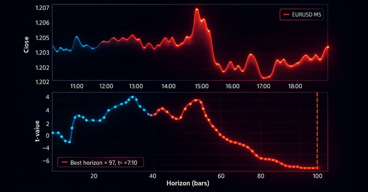
Now let's put trend-scanning to the test using EURUSD M5 data from 2018-01-01 to 2021-12-31. We will use a moving average crossover strategy with MA20 and MA50 as the primary model and apply meta-labeling to the labels generated by the fixed-time horizon, triple-barrier and trend-scanning labeling methods. The trade events (t_events) input to triple_barrier_labels and trend_scanning_labels are determined by the crossovers of the moving averages. To implement meta-labeling with trend-scanning, I only classify a trade as 1 if both the side predicted by the moving average crossover strategy and the trend-scanning labels agree; otherwise, I classify it as 0. I trained a random forest using features that would be predictive for a trend-following model, such as various moving averages, trend features such as ADX, and those obtained by running trend_scanning_labels with lookforward=False (see attached ma_crossover_feature_engine.py). The trend-scanning labels were generated by scanning windows between 5 and 99, by setting span=(5, 100). I used the triple-barrier labeling method to set my stop-loss threshold, but with no profit-taking barrier so that trends run until the horizontal barrier is reached. Below are the relevant settings:
- volatility target = 20-day EWM standard deviation of returns (see get_daily_vol in attached volatility.py).
- profit-taking barrier = 0
- stop-loss barrier = 2
- horizontal barrier = 100
The charts below show trend-scanning in action with the above parameters:


Classification Reports
The results below show the precision, recall and F1-score for various volatility thresholds of the trained random forest classifier, both when unweighted and when the t-values were used as sample weights.
Trend-Scanning Classification Metrics by Volatility Threshold
| 0.0 | 0.05 | 0.1 | 0.2 | 0.3 | ||
|---|---|---|---|---|---|---|
| Class | ||||||
| -1 | precision | 0.505 | 0.489 | 0.486 | 0.448 | 0.428 |
| -1 | recall | 0.545 | 0.382 | 0.408 | 0.440 | 0.413 |
| -1 | f1-score | 0.524 | 0.429 | 0.444 | 0.444 | 0.420 |
| -1 | support | 1043 | 985 | 909 | 752 | 622 |
| 0 | precision | NaN | 0.176 | 0.297 | 0.525 | 0.658 |
| 0 | recall | NaN | 1.000 | 0.926 | 0.875 | 0.858 |
| 0 | f1-score | NaN | 0.299 | 0.449 | 0.656 | 0.745 |
| 0 | support | NaN | 115 | 256 | 566 | 840 |
| 1 | precision | 0.495 | 0.479 | 0.464 | 0.444 | 0.425 |
| 1 | recall | 0.455 | 0.319 | 0.259 | 0.228 | 0.260 |
| 1 | f1-score | 0.474 | 0.383 | 0.332 | 0.301 | 0.323 |
| 1 | support | 1022 | 965 | 900 | 747 | 603 |
| accuracy | 0.500 | 0.387 | 0.407 | 0.482 | 0.550 |
| 0.0 | 0.05 | 0.1 | 0.2 | 0.3 | ||
|---|---|---|---|---|---|---|
| Class | ||||||
| -1 | precision | 0.514 | 0.514 | 0.509 | 0.502 | 0.490 |
| -1 | recall | 0.513 | 0.585 | 0.538 | 0.516 | 0.468 |
| -1 | f1-score | 0.513 | 0.548 | 0.523 | 0.509 | 0.479 |
| -1 | support | 1043 | 945 | 865 | 721 | 596 |
| 1 | precision | 0.504 | 0.513 | 0.506 | 0.501 | 0.485 |
| 1 | recall | 0.505 | 0.442 | 0.478 | 0.487 | 0.508 |
| 1 | f1-score | 0.504 | 0.475 | 0.492 | 0.494 | 0.496 |
| 1 | support | 1022 | 935 | 858 | 719 | 589 |
| accuracy | 0.509 | 0.514 | 0.508 | 0.501 | 0.488 |
| Threshold | Unweighted accuracy | Weighted accuracy |
|---|---|---|
| 0.0 | 0.500 | 0.509 |
| 0.05 | 0.387 | 0.514 |
| 0.1 | 0.407 | 0.508 |
| 0.2 | 0.482 | 0.501 |
| 0.3 | 0.550 | 0.488 |
| Class | Metric | 0.0 | 0.05 | 0.1 | 0.2 | 0.3 |
|---|---|---|---|---|---|---|
| Unweighted model | ||||||
| -1 | f1-score | 0.524 | 0.429 | 0.444 | 0.444 | 0.420 |
| 0 | f1-score | NaN | 0.299 | 0.449 | 0.656 | 0.745 |
| 1 | f1-score | 0.474 | 0.383 | 0.332 | 0.301 | 0.323 |
| Weighted model (t-values as sample weights) | ||||||
| -1 | f1-score | 0.513 | 0.548 | 0.523 | 0.509 | 0.479 |
| 0 | f1-score | N/A (binary classification) | ||||
| 1 | f1-score | 0.504 | 0.475 | 0.492 | 0.494 | 0.496 |
Considerations: when to use weighted vs. unweighted models
Weighted model (t-values as sample weights)
- Emphasize statistically stronger signals: Down-weights noisy or weak labels to reflect evidence strength.
- Stability over peak: Prefer consistent performance across thresholds rather than a single high-accuracy point.
- Production readiness: Robustness and reliability for live trading systems.
- Class imbalance handling: Mitigates dominance of neutral or noisy classes.
Unweighted model
- Explore raw signal quality: Baseline the edge without weighting bias.
- Model neutral/no-trade zones: Retains the flat class (0) where relevant for decision boundaries.
- Research and prototyping: Rapid experimentation before introducing statistical constraints.
- Optimize for peak threshold: If a single operational threshold is targeted and variance is acceptable.
Out of Sample Performance
The results below use uniform bet sizes for trades placed on the occurrence of crossovers of MA20 and MA50 for EURUSD M5 from 2021-12-31 to 2024-12-31. The trend-scanning meta-labels were generated using predictions from a random forest trained with trend-scanning labels with a volatility threshold of 0.05 and with the t-values as sample weights.

Meta‑Labeling vs. Primary Model Performance Comparison (MACrossover 20/50)
| Metric | Fixed Horizon | Triple Barrier | Trend Scanning |
|---|---|---|---|
| Total Return | -12.49% (↓88.4%) | -5.04% (↑34.5%) | 4.53% (↔ 0.0%) |
| Annualized Return | -4.35% (↓92.4%) | -1.71% (↑35.1%) | 1.49% (↔ 0.0%) |
| Sharpe Ratio | -3.72 (↓360%) | -1.66 (↓5.1%) | 2.62 (↑37.3%) |
| Sortino Ratio | -5.09 (↓354%) | -3.66 (↓2.2%) | 4.25 (↑88.5%) |
| Calmar Ratio | -0.285 (↓22.3%) | -0.138 (↑28.9%) | 0.121 (↔ 0.0%) |
| Max Drawdown | 15.27% (↓57.4%) | 12.38% (↑8.8%) | 12.32% (↔ 0.0%) |
| Win Rate | 49.6% (↔) | 40.3% (↑14.5%) | 21.2% (↑88.5%) |
| Profit Factor | 0.96 (↓3.0%) | 0.98 (↔) | 1.04 (↔) |
| Expectancy | -0.0046% (↓332%) | -0.0016% (↓18%) | -0.0762% (↑34%) |
| Kelly Criterion | -0.0206 (↓308%) | -0.0068 (↓14%) | -0.3255 (↑34%) |
Key Insights
The out‑of‑sample results highlight clear differences between the three meta‑labeling approaches:
- Fixed Horizon consistently degraded performance, with negative returns, poor Sharpe and Sortino ratios, and deeper drawdowns. This suggests that rigid time‑based exits are ill‑suited for this strategy.
- Triple Barrier delivered modest improvements in returns and drawdown control, but risk‑adjusted metrics (Sharpe, Sortino) remained weak. It offered some stability but not a decisive edge.
- Trend Scanning stood out with the strongest uplift in risk‑adjusted returns. Sharpe improved by over 37% and Sortino nearly doubled, while drawdowns stayed flat. This indicates that weighting trades by their statistical significance yields more robust and consistent performance.
In practice, Fixed Horizon may be useful only for benchmarking, Triple Barrier for moderate risk control, and Trend Scanning for production‑grade deployment where stability and risk‑adjusted returns matter most.
Extended Meta-Labeled Performance Metrics
| fixed_horizon | triple_barrier | trend_scanning | |
|---|---|---|---|
| total_return | -0.124942 | -0.050359 | 0.045288 |
| annualized_return | -0.043504 | -0.017072 | 0.01487 |
| volatility | 0.888104 | 0.709836 | 0.521126 |
| downside_volatility | 0.649197 | 0.323178 | 0.32075 |
| sharpe_ratio | -3.722773 | -1.66439 | 2.616468 |
| sortino_ratio | -5.092763 | -3.655701 | 4.251009 |
| var_95 | -0.005302 | -0.003206 | -0.002467 |
| cvar_95 | -0.007848 | -0.004445 | -0.003576 |
| skewness | -0.107052 | 1.311478 | 2.165464 |
| kurtosis | 3.459559 | 4.599455 | 14.055488 |
| positive_concentration | 0.000775 | 0.000923 | 0.003244 |
| negative_concentration | 0.000796 | 0.000342 | 0.000683 |
| time_concentration | 0.004943 | 0.004943 | 0.004943 |
| max_drawdown | 0.152723 | 0.123841 | 0.123154 |
| avg_drawdown | 0.021861 | 0.016572 | 0.013556 |
| drawdown_duration | 91 days 05:53:45 | 64 days 09:48:32 | 51 days 23:37:23 |
| ulcer_index | 0.04722 | 0.035056 | 0.029828 |
| calmar_ratio | -0.284854 | -0.137858 | 0.120745 |
| avg_trade_duration | 0 days 06:01:02 | 0 days 07:39:46 | 0 days 04:24:31 |
| bet_frequency | 26 | 66 | 33 |
| bets_per_year | 8 | 21 | 10 |
| num_trades | 2665 | 2665 | 2665 |
| trades_per_year | 888 | 888 | 888 |
| win_rate | 0.495685 | 0.403002 | 0.212383 |
| avg_win | 0.002258 | 0.002348 | 0.002342 |
| avg_loss | -0.002311 | -0.001612 | -0.0016 |
| best_trade | 0.017643 | 0.017643 | 0.017643 |
| worst_trade | -0.01916 | -0.012522 | -0.012522 |
| profit_factor | 0.961558 | 0.983383 | 1.038523 |
| expectancy | -0.000046 | -0.000016 | -0.000762 |
| kelly_criterion | -0.020585 | -0.00681 | -0.325531 |
| consecutive_wins | 6 | 6 | 3 |
| consecutive_losses | 8 | 12 | 3 |
| ratio_of_longs | 0.5 | 0.484375 | 1.0 |
| signal_filter_rate | 0.469546 | 0.469546 | 0.469546 |
| confidence_threshold | 0.5 | 0.5 | 0.5 |
Performance Summary: Labeling Strategies
Trend-Scanning emerges as the most robust strategy across multiple metrics:
- Returns: Only strategy with positive total (+4.5%) and annualized (+1.5%) return.
- Risk-Adjusted Performance: Highest Sharpe (2.62) and Sortino (4.25) ratios, lowest volatility (0.52) and ulcer index (0.03).
- Drawdown Resilience: Shortest drawdown duration (52 days) and lowest average drawdown (0.0136).
- Tail Behavior: Strong positive skew (2.17) and high kurtosis (14.06) suggest asymmetric upside potential.
- Trade Efficiency: Highest profit factor (1.04) despite lowest win rate (21.2%).
- Bias: Fully long-biased (ratio of longs = 1.0), with highest positive concentration (0.0032).
Fixed-Horizon and Triple-Barrier show negative returns and weaker risk-adjusted metrics, though Triple-Barrier offers better downside volatility control and trade frequency.
Conclusion
The trend-scanning methodology proves valuable when properly filtered, though its impact depends on the evaluation framework. Not every trend signal is worth trading—focusing on high-confidence periods delivers far better results.
We’ve progressed from flawed timestamps and rigid labels to an adaptive, probabilistic system that reflects real trading behavior. The key insight is methodological: align your labels with trading reality. Every design choice shapes what your model learns—get it wrong, and complexity won’t save you; get it right, and even simple models can excel.
The future of financial machine learning lies not in more complex algorithms, but in smarter data preparation. With these foundations in place, we’re ready to explore the next frontier: sample weights, model selection, cross-validation, and live deployment. The journey continues.
Warning: All rights to these materials are reserved by MetaQuotes Ltd. Copying or reprinting of these materials in whole or in part is prohibited.
This article was written by a user of the site and reflects their personal views. MetaQuotes Ltd is not responsible for the accuracy of the information presented, nor for any consequences resulting from the use of the solutions, strategies or recommendations described.

- Free trading apps
- Over 8,000 signals for copying
- Economic news for exploring financial markets
You agree to website policy and terms of use
Sorry, but for me the figures don't add up at all:
Total Return +4.53%, Sharpe 2.62, Max DD 12.32%, Win Rate 21.2% and then:
Avg. Win = 0.002342 VS Avg. Loss = -0.0016 -> Expectancy of -0.000762 (-0.076% per trade) is about right
This results in a PR of 0.395 and not 1.038 and with the number of trades of 2665 results in a total return of -203% (2665 * -0.000762)
My God, you still believe these articles about the Machine Learning?
I had a serious flaw in the way I calculated the performance indicators, which I only noticed later. I apologise for this. It's a pity that authors don't have an opportunity to edit their mistakes.
It's none of my business what the service does. Oh, and your translator wrote Ministry of Defence instead of machine learning)))))
I had a serious flaw in the way I calculated the performance indicators, which I only noticed later. I apologise for this. It is a pity that authors do not have the possibility to edit their mistakes.