Feature Engineering for ML (Part 14): Trend-Scanning Features in MQL5

Table of Contents

1. Introduction
2. From O(H·L) to O(H) per Bar
3. Executing the Header Text, Not a Reimplementation
4. The Sign Bug: Same Kernel, Reversed Input, Unreversed Sign
5. What This Means for Part 13
6. Volatility Masking: Why volatility_threshold=0.0 Is a Running Minimum
7. The Indicator: Buffers and the OnCalculate Contract
8. Results: Compiled-Level Performance and Parity
9. The Selection Rule Does Not Select Significance
10. Reading the Features From an EA
11. Conclusion
12. References
13. Attached Files

Introduction

Part 13 wrapped afml.labeling.trend_scanning in a causal-only feature interface, get_trend_scanning_features, that removes the lookforward argument rather than documenting it, because the labeling default is unsafe to call from a feature matrix. This article ports the same causal computation to MQL5 as CTrendScanningFeatures.mqh. Implementing it from first principles instead of relying on the reversal trick used in Python exposed a defect inherited by the Python code: trend_scanning_labels(lookforward=False) returns slope and t-value with the wrong sign.

Section 4 and Section 5 document the finding and its impact on the shipped Part 13 wrapper, with supporting evidence. Section 9 covers a second and separate finding, which concerns the method rather than the code: the rule for choosing among candidate windows does not select the most significant trend, and the t-value it reports cannot be read against the nominal Student-t threshold on price data. Both claims are established by simulation rather than argument.

The rest of the article covers the engineering the port required on its own terms: an O(1)-per-horizon incremental update in place of Part 13's full-window recomputation, a volatility-masking simplification that falls out of the module's own default parameter, and a chart indicator exposing four causal feature buffers through the same iCustom contract used throughout this series.

From O(H·L) to O(H) per Bar

trend_scanning_labels recomputes every candidate window from a Numba kernel that sums the window from scratch: for H horizons averaging length L, that is O(H·L) work per bar. MQL5 has no vectorized reduction to absorb that cost the way NumPy does in the Python original, so a direct translation would pay the full O(H·L) cost as an explicit loop on every bar. CTrendScanningFeatures instead keeps three running sums per horizon and updates them in O(1) per bar.

The identity follows from how the kernel indexes time. A window of length L is fit against a local time index t = 0..L-1, with 0 assigned to the oldest point in the window. Write the three sums the fit needs as:

sum_y(t)  = sum_{i=0}^{L-1} y[t-L+1+i]
sum_y2(t) = sum_{i=0}^{L-1} y[t-L+1+i]^2
sum_ty(t) = sum_{i=0}^{L-1} y[t-L+1+i] * i

When the window slides forward by one bar, every retained point's local index decreases by one and the new point enters at local index L-1. Substituting and collecting terms:

sum_ty(t+1) = sum_ty(t) - sum_y(t) + y_leaving + y_entering * (L-1)
sum_y(t+1)  = sum_y(t)  - y_leaving + y_entering
sum_y2(t+1) = sum_y2(t) - y_leaving^2 + y_entering^2

Each update is four multiplications and a handful of additions, independent of L. mean_t and var_t depend only on L, not on the data, so they are computed once at Init from a closed form rather than re-derived per bar:

const double mean_t = (L - 1) / 2.0;
//--- closed form for sum((t - mean_t)^2), t = 0..L-1: L*(L^2-1)/12
const double var_t  = L * ((double)L * L - 1.0) / 12.0;

The three sums live in a per-horizon struct, and a single ring buffer of length max_horizon + 1 supplies both the entering value (the bar just pushed) and the leaving value (the oldest point of the window one bar back) that every horizon's update needs:

struct HorizonState
  {
   int               L;
   double            mean_t;
   double            var_t;
   double            sum_y;
   double            sum_y2;
   double            sum_ty;
   bool              ready;
  };

A horizon's first valid bar cannot use the incremental update, since there is no previous window to slide from; it is seeded once with a full O(L) sum, as the reference does on every bar. Every bar after that is O(1). Section 8 measures what this is worth in practice, and it is smaller than the O(H·L) versus O(H) description suggests on its own.

Executing the Header Text, Not a Reimplementation

The verification method is the one used for the structural break and fractal engines earlier in this series: CTrendScanningFeatures.mqh is mechanically transformed into compilable C++ (dynamic arrays become std::vector, MQL5 print built-ins are shimmed) and the transformed header text itself is compiled and run, not a hand-written C++ port of the same logic. A driver feeds it a CSV of closes and writes the four output columns; a Python harness runs the identical series through the reference implementation and diffs the two.

g++ -O2 -std=c++17 -I test -o test/run_engine test/run_engine.cpp
python3 test/parity_test.py

Five parameter sets — three span widths, both use_log settings — all matched the Python reference to within 1e-9 on slope and R², and within a relative 3e-5 on t-value. That last tolerance is wider than the others for a specific, checkable reason: a handful of windows in the test data fit a near-perfectly straight line (R² above 0.9999995), and the t-value is computed by dividing by a fitted standard error that is close to zero there. Both implementations are numerically unstable at that degeneracy; the incremental engine's running sums accumulate a few more bits of floating-point drift than a fresh sum over 3-4 points, and that drift is amplified by the same division that makes both versions sensitive in the first place. It is not a logic error, and it is the kind of thing that is easy to miss without a harness that actually executes the shipped code.

The Sign Bug: Same Kernel, Reversed Input, Unreversed Sign

Building the incremental engine independently from the fitting math (rather than from the reversal trick) provided an additional check. Its output was compared bar by bar to trend_scanning_labels(lookforward=False). The magnitudes matched to machine precision. Every slope and t-value had the opposite sign.

The mechanism is in how the backward mode is implemented. It reverses the price series, runs the same forward-only kernel used for labeling, then reverses the order of the results back to bar positions:

y_window = y if lookforward else y[::-1]
t_vals, slopes, r_sq = _window_stats_numba(y_window, hrzn)
if not lookforward:
    t_vals, slopes, r_sq = t_vals[::-1], slopes[::-1], r_sq[::-1]

The kernel always treats index 0 of whatever array it receives as local time zero. In the reversed array, index 0 is the newest original point, not the oldest, so the fitted slope describes how price changes as the local time index increases toward the oldest point; that is a fit against a reversed time axis. Reversing the output order afterward puts each statistic back at the correct bar, but it does not undo the sign consequence of having fit against time running backward.

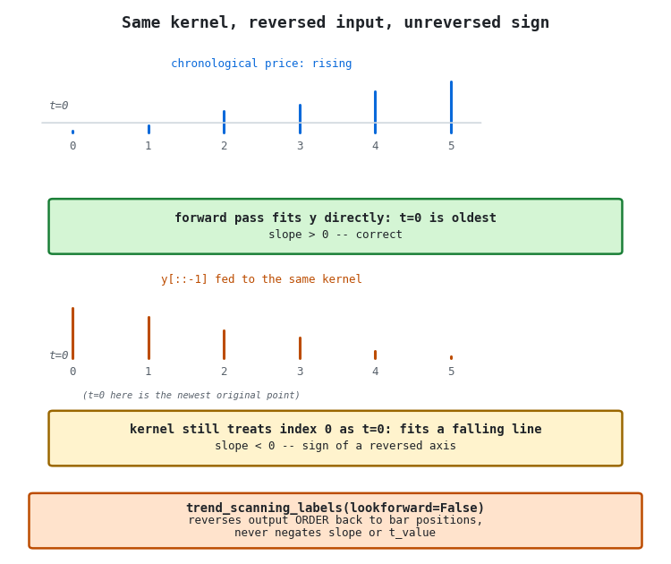
Figure 1. Single-panel illustration of the mechanism behind the sign inversion

• Top: the forward pass fits chronologically rising price directly; local time 0 is the oldest point, and the slope is correctly positive.
• Bottom: the backward pass fits the same six points reversed; local time 0 is now the newest original point, and the same kernel returns a negative slope.
• Base: trend_scanning_labels(lookforward=False) reorders the reversed pass's output back to bar positions but never negates it.

An unambiguous probe confirms it directly. A monotonically rising, lightly noised price series has no legitimate reading under which a causal trend feature should report a negative slope:

close = pd.Series(np.linspace(1.10, 1.14, 40) + noise)

fwd = trend_scanning_labels(close, span=(5,12), lookforward=True)   # slope = +0.001016
bwd = trend_scanning_labels(close, span=(5,12), lookforward=False)  # slope = -0.001016

Across a 1,500-bar synthetic series with three injected drift regimes, the sum of the reference's t-value and the independently-built incremental engine's t-value at every matching bar is zero to within 3e-6, and the corresponding sum for slope is zero to within 2e-13. Window and R², which do not depend on sign, already matched exactly. The forward mode (used correctly for labeling throughout the earlier Blueprint series) does not have this defect: it fits the array directly, with no reversal step to lose a sign across.

What This Means for Part 13

get_trend_scanning_features called trend_scanning_labels(lookforward=False) and returned its slope and t-value unchanged, which means it inherited the inverted sign described in Section 4. The wrapper has been corrected to negate both columns, with the mechanism recorded in its docstring so a future reader does not need to rediscover it:

features = raw.drop(columns=_LABEL_ONLY_COLUMNS)
# the backward call's slope/t_value are measured against a reversed
# time axis and must be negated to read as true chronological direction
features["slope"]   = -features["slope"]
features["t_value"] = -features["t_value"]

The practical impact on Part 13's results is limited. The leak measurement used the forward mode, which is unaffected. The causal hit-rate was computed from sign(t_value) agreement on a symmetric random walk; negating all predictions maps p to 1-p, so a value near 50% remains near 50%. Therefore, the no-leak conclusion is unchanged. The log-defect comparison used the same backward call on both sides of its own comparison, so a shared sign flip cancels out of the agreement and correlation figures reported there.

One figure did depend on the wrapper's absolute sign: the feature panel coloring price by t-value. It has been regenerated with the corrected wrapper and is included in Part 13's attached files. No other figure, table, or numeric claim in Part 13 required a correction.

Volatility Masking: Why volatility_threshold=0.0 Is a Running Minimum

The reference masks any window whose local volatility falls below an expanding quantile of the volatility series itself, and the default for that quantile, in both trend_scanning_labels and Part 13's wrapper, is 0.0. A 0th-percentile quantile is the minimum by definition, and an expanding minimum needs only one running value rather than an order-statistics structure over the whole history:

s.expanding().quantile(0.0) == s.expanding().min()   # identical for every s, verified directly

The engine implements exactly that: one running minimum, updated in O(1) whenever a new volatility value clears the two-point minimum needed for a defined standard deviation. This is the behavior the module actually ships at its default and the only setting Part 13's wrapper exposes. A non-zero volatility_threshold requires a genuine expanding quantile over an unbounded number of past values, which is a materially different, more expensive data structure (an order-statistics tree or a sorted insertion buffer) and is outside the scope of this port. Calling for that setting is a signal this module's masking approach may not be the right fit; the fix belongs in the research design, not in a heavier MQL5 primitive.

The Indicator: Buffers and the OnCalculate Contract

TrendScanViewer.mq5 follows the buffer-class split established in Part 12: a chart-window trend line colored by direction for display, and four calculation buffers — window, slope, t_value, rsquared — that are the only buffers an EA should read.

int horizons[];
CTrendScanningFeatures::BuildHorizons(InpMinHorizon, InpMaxHorizon, horizons);
g_engine.Init(horizons, InpUseLog);

BuildHorizons mirrors list(range(*span)): the maximum is excluded, matching the reference's own convention rather than the more intuitive inclusive reading. Getting this backward would silently drop the widest candidate window from every fit without any error.

The engine is stateful in the same way the fractal engine is: its running sums and ring buffer assume every bar is consumed exactly once, in order. OnCalculate enforces that by stopping one bar short of the array end, so the still-forming bar — which changes on every tick — never reaches the engine:

//--- only closed bars are fed: the forming bar would be reprocessed on
//--- every tick, and the engine consumes each bar exactly once
const int last_closed = rates_total - 2;
TrendScanRow row;

for(int t = g_processed; t <= last_closed; t++)
  {
   ClearBar(t);
   if(!g_engine.ProcessBar(close[t], row))
      return(0);
   StoreRow(t, row, close[t]);
   g_processed = t + 1;
  }

Results: Compiled-Level Performance and Parity

A first attempt at measuring the incremental design's benefit compared pure-Python implementations of both paths, and the two came out within a few percent of each other. That result did not survive scrutiny. The naive side used NumPy array slicing, whose C-level vectorized reduction absorbs most of an O(L) window sum's cost regardless of L for the window sizes here, and the comparison ended up measuring interpreter and array-allocation overhead shared by both paths rather than the sum computation the incremental design actually changes.

The fair comparison is at the level MQL5 actually runs at: both paths compiled, doing identical downstream work (slope, SSE, R², t-value, and the argmax over horizons), differing only in how the three running sums are obtained.

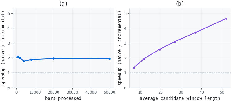
Figure 2. Two-panel illustration of the measured speedup, both paths verified to agree numerically

• Panel (a): speedup versus series length at the span used throughout this series, span(5,20); roughly flat, since both implementations are O(bars) overall and only the per-bar constant differs.
• Panel (b): speedup versus average candidate window length at a fixed 50,000 bars, rising from 1.35x at span(5,10) to 4.65x at span(5,100).

For the span used throughout this series, span(5,20), the incremental design yields about a 2× speedup, not an order-of-magnitude improvement. The downstream statistics (slope, SSE, R², t-value) cost the same either way and are not small next to a short window's sum; the saving is concentrated in the sum computation itself, and that computation is a shrinking share of the total as L grows, which is exactly the trend panel (b) shows. Every reported number in both panels comes from the two implementations agreeing to a relative difference under 1e-6 on the same run, printed alongside the timing so a discrepancy could not be posted as a legitimate result by accident.

Numerical parity between the executed MQL5 header and the Python reference, across all four output columns:

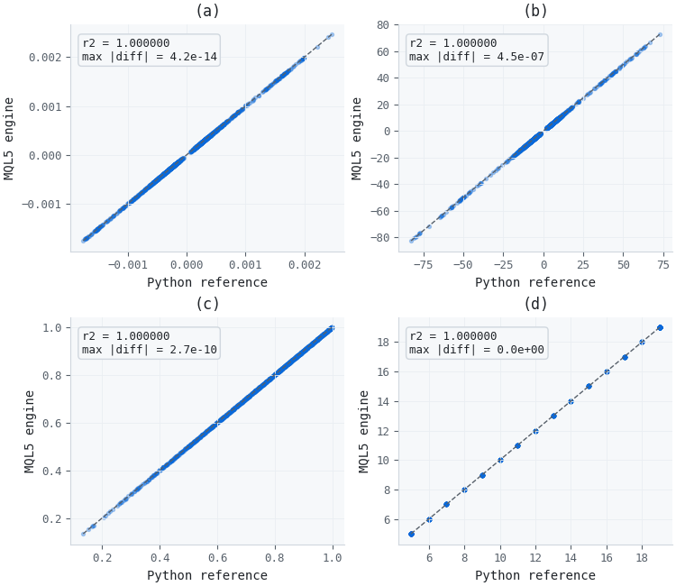
Figure 3. Four-panel illustration of numerical agreement between the two implementations

• Panel (a): slope.
• Panel (b): t-value.
• Panel (c): R².
• Panel (d): chosen window length, matching on every bar.

The Selection Rule Does Not Select Significance

The port reproduces the reference implementation, and that includes reproducing its rule for choosing among candidate windows: fit every horizon, keep the one with the largest absolute t-value. Section 5.4 of Machine Learning for Asset Managers introduces that rule with a specific justification, namely that it labels each observation according to the most statistically significant trend among the periods evaluated. Building a calibration harness for the indicator showed that the rule does not accomplish what that sentence claims.

The reason is that the t-value is not a quantity that can be compared across windows of different length. A t-statistic is referred to a Student-t distribution with L - 2 degrees of freedom, and the shape of that distribution changes with L. A five-bar window has three degrees of freedom and a distribution with heavy tails; a forty-bar window has thirty-eight and a distribution close to normal. The same numerical t-value therefore carries a different amount of evidence depending on which window produced it, and taking the maximum over raw t-values systematically favors the shortest windows in the span.

A deterministic series quantifies the size of the effect. Take y[i] = 100 + 0.05i + 3sin(0.3i), fit on log price, and evaluate all windows from 5 to 40 bars ending at bar 199. The largest absolute t-value is -12.840, produced by the five-bar window. Its two-sided p-value on three degrees of freedom is 1.02e-3. The twenty-bar window produces a t-value of only +6.572, but on eighteen degrees of freedom that carries a p-value of 3.57e-6. The window the prescribed rule discards is roughly 286 times more significant than the window it selects.

The two windows also disagree about which way price is moving. The five-bar fit is falling and the twenty-bar fit is rising, so on this bar the rule as published reports a downtrend where the more significant reading is an uptrend. This is not a pathological construction; it happens whenever a short reversal is embedded in a longer move, which on intraday data is common.

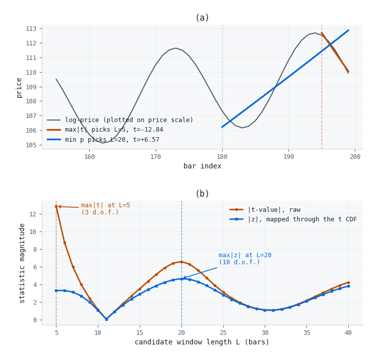
Figure 4. Two-panel illustration of the two selection rules reaching opposite conclusions on one bar

• Panel (a): the five-bar window chosen by the raw rule and the twenty-bar window chosen after length correction, both fitted on the same final bar and pointing in opposite directions.
• Panel (b): the profile of both statistics across the candidate span, showing raw absolute t-value peaking at the short end while the corrected statistic peaks near twenty bars.

The correction is to put every candidate on a common scale before comparing them. Mapping each t-value through its own t distribution produces a p-value, and mapping that p-value back through the standard normal quantile produces a score whose units no longer depend on window length. MQL5 has no gamma function among its built-ins, so the t distribution function has to be supplied. A Lanczos log-gamma feeding a regularized incomplete beta is sufficient and is self-contained:

//+------------------------------------------------------------------+
//| TSS_TTwoSidedP: two-sided p-value for a t-statistic              |
//+------------------------------------------------------------------+
double TSS_TTwoSidedP(const double t, const int df)
  {
   if(df <= 0)
      return(1.0);
   return(TSS_Betai(0.5 * df, 0.5, df / (df + t * t)));
  }

//+------------------------------------------------------------------+
//| TSS_SignedZ: put a t-statistic on the standard-normal scale      |
//+------------------------------------------------------------------+
double TSS_SignedZ(const double t, const int df)
  {
   double p = TSS_TTwoSidedP(t, df);
   if(p < 1.0e-300)
      p = 1.0e-300;
   if(p > 1.0)
      p = 1.0;
   const double z = -TSS_InvNormCdf(0.5 * p);
   return(t >= 0.0 ? z : -z);
  }

The selection loop then compares MathAbs(TSS_SignedZ(t_value, L - 2)) in place of MathAbs(t_value). Everything else in the engine is unchanged, because the per-horizon fitting math is not what was wrong.

The engine attached to this article keeps the raw rule as its default. That is deliberate: Section 3 and Section 8 establish parity against the Python reference, and changing the selection rule would break the property those sections verify. The corrected comparison is supplied as a separate include so it can be switched on without disturbing the parity result.

The nominal threshold is a second, larger problem

Correcting the comparison across windows does not make the resulting p-value trustworthy, because the p-value rests on an assumption that price data violates. Ordinary least squares assumes serially independent residuals. Price levels are integrated of order one, so a fitted trend leaves residuals that are strongly autocorrelated, the standard error is understated, and the t-value is inflated. This is the spurious regression problem described by Granger and Newbold in 1974, and it applies to a trend fitted to prices exactly as it applies to a regression between two unrelated random walks.

Simulation puts a number on it. Generating twenty thousand driftless random walks of 260 observations and scanning windows from 5 to 40 bars on each, the 95th percentile of the maximum absolute t-value is 21.04 and the 99th percentile is 28.24. The nominal two-sided five percent threshold on thirty-eight degrees of freedom is 2.024. Applying that nominal threshold to these trendless series flags 99.94 percent of bars as significantly trending.

The same experiment run on independent noise rather than a random walk returns a 95th percentile of 4.22 for the scan and 2.03 for a single forty-bar window. That second figure matching the nominal 2.024 almost exactly is the control: it confirms the t-value calculation in the engine is correct, and that the inflation seen on price-like data is a property of the data rather than an error in the implementation.

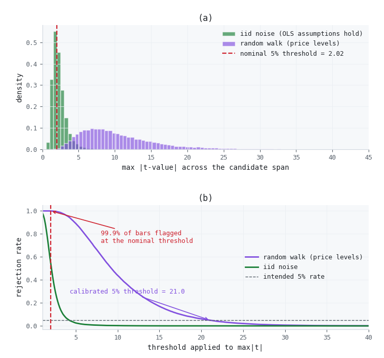
Figure 5. Two-panel illustration of the scan statistic under a null containing no trend

• Panel (a): distribution of the maximum absolute t-value across the candidate span for independent noise and for a random walk, against the nominal five percent threshold.
• Panel (b): fraction of trendless bars declared significant as a function of the threshold applied, with the calibrated five percent point marked.

Decomposing the inflation is worth doing, because it changes which remedy is appropriate. A single forty-bar window on a random walk already reaches a 95th percentile of 17.32. Scanning thirty-six windows and keeping the extreme value raises that only to 21.04, a factor of about 1.21. Almost all of the distortion comes from fitting a trend to an integrated series, and only a small residual comes from searching over horizons. A multiple-testing adjustment on the number of horizons, such as a Bonferroni or Sidak correction, would therefore address the smaller of the two effects and leave the larger one untouched.

What does work is simulating the statistic that is actually reported, on data generated with no trend, using the same candidate span the engine is configured with, and taking the upper quantiles of that simulated distribution as the thresholds. The procedure is short: draw a driftless random walk of max(L) increments, compute the statistic on every trailing window in the span, record the maximum, repeat several thousand times, and sort. Because the statistic at one bar depends only on the trailing max(L) observations, each replication needs no more history than that, which makes a few thousand replications cheap enough to run once at initialization. A fixed seed keeps the resulting thresholds reproducible across restarts.

Two caveats belong with this. A driftless random walk is a convenient null rather than a correct model of price, so the thresholds it produces are a calibration and not an exact test; a null with fat tails or volatility clustering would shift them. And a calibrated threshold says only that the observed trend is larger than a trendless series of the same length usually produces. It says nothing about whether the trend continues on the next bar.

Reading the Features From an EA

As with the fractal viewer of Part 12, only the confirmation-bar buffers are safe to read, and shift 1 rather than shift 0 is the correct read point, since shift 0 is the still-forming bar the indicator deliberately leaves empty:

int handle = iCustom(_Symbol, _Period, "TrendScanViewer", 5, 20, true);

double t_value[];
double window[];
if(CopyBuffer(handle, 4, 1, 1, t_value) < 1)
   return;
if(CopyBuffer(handle, 2, 1, 1, window) < 1)
   return;

//--- compare on the length-corrected scale, against a threshold
//--- calibrated for this candidate span rather than the nominal 2.0.
//--- See Section 9: the nominal threshold flags almost every bar.
const int    df    = (int)window[0] - 2;
const double score = TSS_SignedZ(t_value[0], df);

if(score > g_calibrated_crit95)
   OpenLong();

A positive t_value now means what it should: the fitted trend, using only bars up to and including the current one, is rising. That was not true of the equivalent Python call before the correction in Section 5, which is the reason this section exists at all rather than being a one-line footnote.

The threshold in that example is a calibrated value, not the nominal 2.0 a t-statistic would normally be compared against. Section 9 explains why that comparison flags essentially every bar on price data. The window buffer is read here for a second reason beyond diagnostics: the degrees of freedom needed to interpret the t-value depend on which window was selected, so the two values have to be read together.

Conclusion

The incremental design ported cleanly: the same three running sums that make the O(1) update possible in MQL5 are exactly the quantities the fitting math needs, verified by executing the shipped header text as C++ rather than trusting a parallel reimplementation. Its performance benefit is real but modest at the span this series has used, roughly 2x, growing with the width of the candidate span because the per-horizon statistics that do not benefit from the incremental update become a smaller share of the total as windows lengthen.

The more consequential finding came from building that verification independently rather than from optimizing it. trend_scanning_labels(lookforward=False) fits a reversed time axis and never corrects for it, so its slope and t-value carry the wrong sign; Part 13's feature wrapper inherited that defect and has been corrected, as Section 5 sets out. The forward mode used for labeling throughout the earlier Blueprint series does not share this defect. Readers running any pipeline that called the backward mode directly, rather than through the corrected wrapper, should check the sign of anything downstream of it.

A second finding came out of building the indicator rather than the engine, and it concerns the method rather than any implementation of it. Choosing the candidate window by the largest absolute t-value does not choose the most significant trend, because t-values from windows of different length are referred to distributions with different degrees of freedom; on the worked example in Section 9 the rule selects a window roughly 286 times less significant than one it discards, and reports the opposite trend direction. Separately, the t-value itself cannot be read against the nominal threshold on price data at all: under a driftless random walk containing no trend, 99.94 percent of bars exceed the nominal five percent value. Almost all of that inflation comes from fitting a trend to an integrated series rather than from searching over horizons, which is why a multiple-testing adjustment on the horizon count is the wrong remedy and simulating the reported statistic under a trendless null is the right one.

This is the second installment in this series where the causal, MQL5-facing half of a feature family surfaced a defect the Python half had already shipped: Part 12 caught a series-indexed feed silently inverting the fractal confirmation lag, and this article caught a sign inversion in trend-scanning's own labeling module. Verifying a port by executing it, rather than assuming the reference it is checked against is correct, has now paid for itself twice in this series.

References

1. Lopez de Prado, M. Advances in Financial Machine Learning: Lecture 3/10.
2. Lopez de Prado, M. (2018). Advances in Financial Machine Learning. Wiley.
3. Lopez de Prado, M. (2020). Machine Learning for Asset Managers, Section 5.4. Cambridge University Press.
4. Granger, C. W. J. and Newbold, P. (1974). Spurious regressions in econometrics.Journal of Econometrics, 2(2), 111-120.

Attached Files

	File	Location	Description
1.	CTrendScanningFeatures.mqh	MQL5\Include\Features	Incremental engine. Init, Reset, ProcessBar for bar-by-bar use, and the static BuildHorizons helper.
2.	TrendScanViewer.mq5	MQL5\Indicators\Features	Chart indicator with one display plot and four calculation buffers, addressable through iCustom.
3.	TrendScanValidation.mq5	MQL5\Scripts\Features	Exports bars and all four features to CSV at sixteen significant digits.
4.	incremental_scanner.py	MQL5\Files\Features	Independent incremental reference used to cross-check the MQL5 port; not a copy of the MQL5 code translated back.
5.	validate_trend_scan.py	MQL5\Files\Features	Parity checker for the MQL5 export. Reports maximum absolute deviation per column and a relative check for t-value.
6.	trend_scanning_features.py	MQL5\Files\Features	Part 13's wrapper, corrected per Section 5. Superseded copy for anyone tracking the diff.
7.	TrendScanSignificance.mqh	MQL5\Include\Features	Section 9 add-on. Lanczos log-gamma, regularized incomplete beta, two-sided t p-value, inverse normal, and the random-walk threshold calibrator. Leaves the parity-verified engine untouched.
8.	selection_rule_evidence.py	MQL5\Files\Features	Reproduces every number quoted in Section 9 and regenerates Figures 4 and 5, including the decomposition of the inflation into its two sources.