

Building Volatility Models in MQL5: Implementing the APARCH Volatility Process
 141
141
 0
0

Contents
- Introduction
- The Problem with Fixing Delta
- Asymmetric Power ARCH
- APARCH MQL5 Implementation
- SLSQP Solver Updates
- Nesting Existing Models with APARCH
- The APARCH Volatility Indicator
- Benchmarking APARCH
- Conclusion
Introduction
The GARCH-like volatility processes implemented so far are defined by configurable lag lengths and fixed power parameters. This aligns with standard specifications of ARCH, GARCH, EGARCH, GJR-GARCH, HARCH, TARCH, and FIGARCH, where the framework fixes the exponent before optimization begins. If an alternative, optimal exponent exists, no diagnostic flags the issue; the optimizer simply operates within the assigned constraint, silently narrowing the parameter space. In asymmetric volatility models, the exponent's interaction with the asymmetry term can directly alter parameter estimation. This limitation belongs to the same class of design trade-offs that motivated EGARCH's log-variance formulation: a restriction adopted for operational convenience that quietly restricts the universe of candidate models.
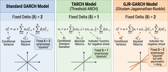
Ding, Granger, and Engle proposed a framework that jointly estimates the power parameter with the other model coefficients: the Asymmetric Power ARCH (APARCH) model. This article implements APARCH as the CAparchProcess class in the CVolatilityProcess hierarchy. It explains why fixing the power term is unnecessarily restrictive, then describes the MQL5 implementation (recursion, bounds, stationarity constraints, and initialization).
It also summarizes optimizer changes. Finally, it demonstrates nesting by constraining APARCH to reproduce close estimates of GARCH and GJR-GARCH conditional volatility before presenting the APARCH volatility indicator built on the new process. It should be noted that this text does not claim that APARCH is a superior modeling framework; it merely suggests that it is a useful addition to the library, providing an alternate approach to conditional volatility modeling. This will be investigated by a script comparing the model's performance in out-of-sample testing.
The Problem with Fixing Delta
Traditional GARCH models dictate that conditional variance depends strictly on squared returns. However, empirical studies indicate that the autocorrelation of squared returns drops off faster than that of absolute returns or intermediate powers. The delta parameter controls the power to which conditional volatility is raised before being modeled linearly. Standard GARCH fixes delta at 2 to model conditional variance, whereas TARCH implicitly uses a delta of 1 to model standard deviation. Rather than assuming a specific response to shocks, freeing delta allows the data to reveal its optimal functional form. Empirically, financial returns often fit better with a delta closer to 1 than 2—meaning volatility responds more linearly to shock magnitudes than classical specifications assume.
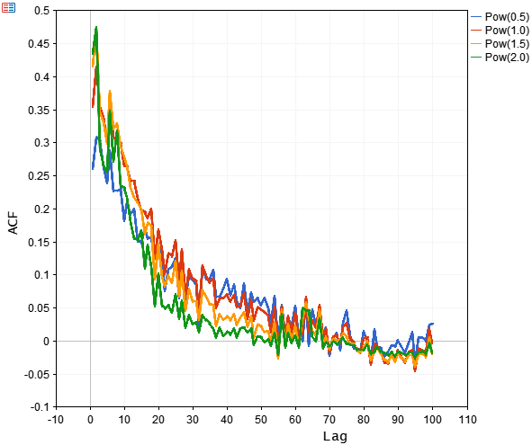
The empirical observation that absolute returns often display higher and longer-lasting serial autocorrelation than squared returns is known as the Taylor Effect. While the Taylor Effect provides compelling motivation to explore alternative power transformations, it does not guarantee that a given delta estimate captures the true underlying volatility dynamics. To illustrate the Taylor effect, the script Taylor_Effect_Visualization.mq5 fetches historical market data, calculates return transformations across power parameters {0.5, 1.0, 1.5, 2.0}, and plots their autocorrelation decay functions over 100 lags.
#include<aparch\Arch\univariate\acf.mqh>
//--- input parameters
input datetime         StartDate = D'2025.01.01';      //--- Historical capture anchor stop date
input ulong            HistoryLen = 5000;              //--- Total historical data bars to request
//---
ulong      Max_Lags = 100;
double     Powers_Start = 0.5;
double     Powers_Stop = 2.0;
double     Powers_Step = 0.5;
//+------------------------------------------------------------------+
//| Script program start function                                    |
//+------------------------------------------------------------------+
void OnStart()
  {
//---
   vector prices;
//--- --- Historical Data Fetch ---
//--- Pull close prices directly into an array using native vector operations
   if(!prices.CopyRates(NULL,PERIOD_CURRENT, COPY_RATES_CLOSE, StartDate, HistoryLen))
     {
      Print(" failed to get close prices for ", _Symbol, ". Error ", GetLastError());
      return;
     }
//--- --- Transform Prices to Returns ---
//--- Map closing prices to logarithmic space
   prices = log(prices);
//--- Compute log returns: r_t = ln(P_t) - ln(P_{t-1})
   vector returns = np::diff(prices) * 100.0;
//--- Demean the data and
   vector demeaned_returns = returns - returns.Mean();
   vector abs_returns = fabs(demeaned_returns);
   vector powers = np::arange(Powers_Start,Powers_Stop+Powers_Step,Powers_Step);
//--- Compute the Autocorrelation at different powers of absolute returns
//--- This is the data plotted on the y-axis of the graph
   vector t_series;
   ACFResult acf_result;
   vector acf_results[];
   ArrayResize(acf_results,(int)powers.Size());
   for(ulong i = 0; i<powers.Size(); ++i)
     {
      t_series = pow(abs_returns,powers[i]);
      acf_result = acf(t_series,Max_Lags,0.05,true,true,false,true);
      acf_results[i] = np::sliceVector(acf_result.acf,1);
     }
//--- The data on x-axis of plot
   vector lags = np::arange(Max_Lags,1.0,1.0);

//--- Plot the graph
//--- Prepare curve labels
   string ylabels[];
   ArrayResize(ylabels,(int)powers.Size());
   for(uint i = 0; i<ylabels.Size(); ++i)
      ylabels[i] = "Pow("+string(powers[i])+")";
//--- Show the graphic
   np::plotxys(lags,acf_results,ylabels,"Autocorrelation Drop-off","Lag","ACF",false,0,0,0,0,750,500,true,3,CURVE_LINES,30);
//---
   return;
  }
Running the script on a daily S&P 500 chart yielded the following graphic:
Asymmetric Power ARCH
The APARCH conditional volatility equation is defined as follows:
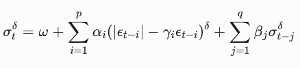
Four groups of parameters govern the process. Omega is the baseline scale term, expressed in the model's power-transformed units rather than raw variance units; it plays the same anchoring role as omega in GARCH and EGARCH. The beta coefficients measure persistence—governing how slowly a shock to the power-transformed variance decays.
Unlike standard GARCH processes where simple bounds on the autoregressive sum suffice, the covariance stationarity of an APARCH process depends on a joint condition across the parameters as well as the moments of the underlying innovation distribution—specifically requiring that the combined persistence from past variance and the expected asymmetric, power-transformed residual shock stays below 1 to prevent volatility from exploding over time. The alpha coefficients scale the (shifted, powered) magnitude of past shocks, playing the same role as alpha in GARCH. What differs is what gets scaled: rather than the raw squared or absolute residual, the term scaled by alpha is itself shock-dependent through gamma before any exponent is applied.
The gamma coefficients introduce asymmetry into the model. When gamma = 0, the shift term vanishes, treating positive and negative shocks identically and collapsing the model back to a symmetric Power-ARCH specification. When gamma > 0, a negative shock impacts volatility more heavily than a positive shock of equal magnitude, meaning negative returns generate more volatility—reflecting the familiar equity leverage effect. A negative gamma reverses this, producing the inverse leverage effect more commonly seen in commodity markets. Gamma is bounded within the open interval (-1, 1). When outside this range, the shift term can turn negative for a specific shock sign, which is not meaningful once raised to a fractional power.
Finally, delta is the exponent, estimated jointly with every other parameter rather than fixed by the user. A delta close to 2 recovers models built around squared residuals, while a delta close to 1 recovers models built around absolute residuals. Intermediate values, which are common in equity estimation, indicate that neither standard convention describes the data particularly well. Because delta, alpha, gamma, and beta are estimated jointly, APARCH nests several existing models. For example, delta = 2 and gamma = 0 with one alpha and one beta will reproduce GARCH(1,1). Delta = 1 with one asymmetry lag reproduces TARCH. Setting q = 0 yields an asymmetric power ARCH model without persistence. This nesting property is used later in the article to validate the new implementation against previously verified library code.
APARCH MQL5 Implementation
The implementation follows the pattern established by CVolatilityProcess derivatives. The enum member VOL_APARCH is added to ENUM_VOLATILITY_MODEL in base.mqh. New members are added to ArchParameters: aparch_delta maps to the value of delta and acts as a flag signaling whether this parameter should be refined by the optimizer. By default, it is set to EMPTY_VALUE. When set to any value other than EMPTY_VALUE, delta is treated as fixed and will not be refined alongside other model coefficients. Valid values for a fixed delta lie in the range [0.05, 4.0]; values outside this range trigger a runtime error.
//+------------------------------------------------------------------+
//| Configured conditional volatility structure models                |
//+------------------------------------------------------------------+
enum ENUM_VOLATILITY_MODEL
  {
   VOL_CONST = 0, // Homoskedastic variance baseline profiles
   VOL_ARCH,      // Autoregressive Conditional Heteroskedasticity (Linear lag squares mapping)
   VOL_AVARCH,    // Absolute Value ARCH framework configurations
   VOL_AVGARCH,   // Absolute Value GARCH process modeling variations
   VOL_TARCH,     // Threshold ARCH / ZARCH threshold tracking handling asymmetric volatility shocks
   VOL_GARCH,     // Generalized ARCH processes combining structural innovations and past variance memory
   VOL_GJR_GARCH, // Glosten-Jagannathan-Runkle GARCH tracking sign-dependent asymmetric leverage adjustments
   VOL_HARCH,     // Heterogeneous ARCH handling multi-scale localized aggregate time horizons
   VOL_FIGARCH,   // Fractionally Integrated GARCH mapping long-memory long-term decay processes
   VOL_EGARCH,    // Exponential Generalized ARCH processes
   VOL_APARCH     // Asymmetric Power ARCH volatility process
  };
The second new ArchParameters member is aparch_common_asym, a boolean that restricts all asymmetry terms to share a single asymmetry coefficient when set to true (it defaults to false). Restricting all gammas to a single common value promotes parsimony at the expense of flexibility while keeping APARCH's nesting structure clean and comparable to other delta-fixed GARCH-like models.
//+------------------------------------------------------------------+
//| Comprehensive specification payload structure for ARCH models   |
//+------------------------------------------------------------------+
struct ArchParameters
  {
   // --- Data & Core Configuration
   vector            observations;       // Vector tracking endog target returns data series
   matrix            exog_data;          // Matrix tracking exogenous external regressor blocks
   vector            mean_lags;          // Vector defining selected conditional mean lag lengths

   ENUM_MEAN_MODEL   mean_model_type;    // Specified mean structural method profile reference
   ENUM_VOLATILITY_MODEL vol_model_type; // Specified volatility variance framework engine reference
   ENUM_DISTRIBUTION_MODEL dist_type;    // Specified baseline conditional probability density model

   ulong             holdout_size;       // Out-of-sample data truncation window count bounds
   bool              is_rescale_enabled; // Scale switch flag to normalize inputs to unit variances
   double            scaling_factor;     // Internal scale factor used for numerical optimization convergence

   // --- Mean Model Parameters
   bool              include_constant;   // Conditional mean calculation model constant flag
   bool              use_har_rotation;   // Flag enabling volatility horizon mapping blocks rotations

   // --- Volatility Process Parameters (GARCH/ARCH)
   int               vol_rng_seed;       // Random initialization seeding value used for variance simulations
   ulong             garch_p;            // Shock innovations lag loop parameter allocation bounds (ARCH)
   ulong             garch_o;            // Asymmetric conditional volatility component bounds (Leverage)
   ulong             garch_q;            // Historical tracking persistence variance memory depth (GARCH)
   double            vol_power;          // Exponent index scaling term used in variance conversions
   ulong             figarch_truncation; // Expansion step cutoff limit boundary tracking fractional integration weights
   vector            harch_lags;         // Structural lookback specification arrays targeted by HARCH processes

   double            aparch_delta;       // Value to use for a fixed delta in the APARCH model. If not provided (empty value)
                                         // the value of delta is jointly estimated
                                         // with other model parameters. User provided delta is restricted
                                         // to lie in [0.05, 4.0].
   bool              aparch_common_asym; // Restrict all asymmetry terms to share the same asymmetry
                                         // parameter. If False (default), then there are no restrictions
                                         // on the ``o`` asymmetry parameters
A new aparch_recursion() function is added to recursions.mqh. Whereas garch_recursion() receives pre-transformed power residuals and a separate sign vector, aparch_recursion() receives the raw residual series directly. This is because the shift-then-power transformation cannot be precomputed independently of the asymmetry coefficient; the coefficient is estimated dynamically during optimization rather than serving as a structural constant.
Pre-sample values are initialized using the scalar backcast expressed on the variance scale, rather than being pre-transformed. The recursion explicitly scales backcast inside the loop—to seed initial shock terms and to initialize pre-sample power-transformed conditional variances.
//+------------------------------------------------------------------+
//| Compute variance recursion for APARCH models                     |
//+------------------------------------------------------------------+
vector aparch_recursion(vector& parameters, vector& resids, vector& abs_resids, vector& sigma2, vector& sigma_delta, ulong p, ulong o, ulong q, ulong nobs, double backcast, matrix& var_bounds)
  {
   double delta = parameters[1 + p + o + q];
   double shock = 0;
   for(long t = 0; t<long(nobs); ++t)
     {
      sigma_delta[t] = parameters[0];
      for(long j = 0; j<long(p); ++j)
        {
         if((t - 1 - j) < 0)
            shock = pow(backcast,0.5);
         else
           {
            shock = abs_resids[t - 1 - j];
            if(long(o) > j)
               shock -= parameters[1 + p + j] * resids[t - 1 -j];
           }
         sigma_delta[t] += parameters[1 + j] * pow(shock,delta);
        }
      for(long j = 0; j<long(q); ++j)
        {
         if((t - 1 - j) < 0)
            sigma_delta[t] += parameters[1 + p + o + j] * pow(backcast,delta/2.);
         else
            sigma_delta[t] += parameters[1 + p + o + j] * sigma_delta[t - 1 - j];
        }
      sigma2[t] = pow(sigma_delta[t],(2.0/delta));
      sigma2[t] = bounds_check(sigma2[t], var_bounds.Row(t));
      sigma_delta[t] = pow(sigma2[t],(delta/2.));
     }
   return sigma2;
  }
The class CAparchProcess is defined in volatility.mqh as a derivative of CVolatilityProcess. Its protected members m_p, m_o, and m_q hold the ARCH, asymmetry, and GARCH orders, respectively, while m_delta holds delta—either fixed (checked against the [0.05, 4.0] range used in academic literature) or estimated jointly, as flagged by the EMPTY_VALUE constant. The m_asym flag exposes whether all asymmetry terms are tied to a single shared value. The constructor activates this flag only when an asymmetry order is specified. When active, the _initialize() method collapses the internal asymmetry order to a single slot, ensuring the optimizer only searches over one gamma rather than one per lag. This directly reduces the parameter count and shrinks the dimensionality of the estimation problem.
//+------------------------------------------------------------------+
//| APARCH process                                                   |
//| Models volatility as a sum of lags over different frequencies    |
//+------------------------------------------------------------------+
class CAparchProcess: public CVolatilityProcess
  {
protected:
   ulong               m_p;            // Order of the ARCH component
   ulong               m_o;            // Order of Asymmetry component
   ulong               m_q;            // Order of the GARCH component
   double              m_delta;        // Value to use for a fixed delta in the APARCH model.
   bool                m_asym;         // Restrict all asymmetry terms to share the same asymmetry true or false
   bool                m_est_delta;    // Internal flag on whether to estimate delta or not
   bool                m_repack;       // Whether to repack or reformat the model parameters;
   vector              m_parameters;   // Model parameters
   vector              m_sigma_delta;  // Sigma delta

   vector            _repack_parameters(vector& parameters);

   matrix            _product(vector& one, vector& two, vector& three,vector& four);
   //--- Verify if the requested forecasting method is mathematically valid
   //--- Analytic methods require specific power=2.0 structures for multi-step persistence
   virtual bool        _check_forecasting_method(ENUM_FORECAST_METHOD method, ulong horizon);
   //--- Analytic multi-step volatility forecasts from the model
   virtual VarianceForecast _analyticforecast(vector& parameters, vector &resids, vector &backcast, matrix &varbounds, long _start, ulong horizon);
   //--- Simulation of paths helper method
   bool              _simulate_paths(ulong m, vector& parameters, ulong horizon, matrix& std_shocks, matrix& sigma_delta, matrix& shock, matrix& abs_shock, matrix& f_out, matrix& p_out, matrix& s_out, ulong row_index);
   //--- Simulation-based volatility forecasts from the model
   virtual VarianceForecast _simulationforecast(vector& parameters, vector &resids, vector &backcast, matrix &varbounds, long _start, ulong horizon, ulong simulations, BootstrapRng &rng);

   //--- Initialize class members
   virtual bool      _initialize(ENUM_VOLATILITY_MODEL volmodel = WRONG_VALUE, bool updateable = true, bool closedform = false, ulong nparams = 0, string name = NULL, int seed = 0, ulong p = 0, ulong o = 0, ulong q = 0, double power = EMPTY_VALUE, long start = 0, long stop = -1, ulong bootstrap_obs = 100);

public:
                     CAparchProcess(void)

                     CAparchProcess(ulong p, ulong o, ulong q, double delta, bool common_asym, int seed, long start, long stop, ulong boot);

   //--- Return value of delta in the model
   double            delta(void);

   //--- Return whether all asymmetric terms share the same coefficient
   bool              common_asym(void);

   //--- Returns starting values for the ARCH model using a grid-search heuristic initialization
   virtual vector    startingValues(vector& resids);


   //--- Returns boundary matrix structures for parameters optimization constraints
   virtual matrix    bounds(vector& resids) override

   //--- Compute the variance for the ARCH model
   virtual vector    computeVariance(vector& parameters, vector& resids, vector& _sigma2, vector& _backcast, matrix& varbounds);


   //--- Construct parameter constraints arrays for parameter estimation (Boundary bounding vectors)
   virtual Constraints constraints(void) override


   //--- Simulate data paths from the model structure
   virtual matrix      simulate(vector& parameters, ulong _nobs, BootstrapRng &rng, ulong burn = 500, double initial_value = NULL);


   //--- Names of model parameters
   virtual string       parameterNames(void);

  };
The startingValues() method extends the grid-search heuristic used by CGarchProcess and CEgarchProcess with an additional dimension for delta, evaluating candidate combinations of alpha, gamma, beta, and delta against the Gaussian log-likelihood and selecting the highest-scoring combination—exactly as existing classes do for their three-dimensional grids.
//--- Returns starting values for the ARCH model using a grid-search heuristic initialization
virtual vector    startingValues(vector& resids) override
  {
   ulong p = m_p;
   ulong o = m_o;
   ulong q = m_q;

   vector alphas = {0.03, 0.05, 0.08, 0.15};
   vector alpha_beta = {0.8, 0.9, 0.95, 0.975, 0.99};

   vector gammas;
   if(m_o>0)
     {
      gammas.Resize(3);
      gammas[0] = -0.5;
      gammas[1] = 0.;
      gammas[2] = 0.5;
     }
   else
      gammas = vector::Zeros(1);


   vector deltas;
   if(m_est_delta)
     {
      deltas.Resize(3);
      deltas[0] = 0.5;
      deltas[1] = 1.2;
      deltas[2] = 1.8;
     }
   else
     {
      deltas.Resize(1);
      deltas[0] = m_delta;
     }

   matrix agbs = _product(alphas,gammas,alpha_beta,deltas);

   double target = 0.0;

   vector svs[];
   ArrayResize(svs, int(agbs.Rows()));
   matrix vb = varianceBounds(resids);
   vector llfs = vector::Zeros(agbs.Rows());
   ulong est_delta = ulong(m_est_delta);
   vector bc = backCast(resids);
   double alpha,gamma,ab,delta,scale;
// Evaluate Log-Likelihood for each combination in the grid
   for(uint i = 0; i < svs.Size(); ++i)
     {
      vector row = agbs.Row(i);
      alpha = row[0];
      gamma = row[1];
      ab = row[2];
      delta = row[3];
      //---
      target = (pow(fabs(resids),delta)).Mean();
      scale = (pow(resids,2.)/pow(target,2.0/delta)).Mean();
      target*=pow(scale,delta/2.0);
      // Construct starting vector: constant omega + lags
      vector sv = (1. - ab) * target * vector::Ones(p + o + q + 1 + est_delta);
      for(ulong j = 1; j<1+p; sv[j] = alpha/p, ++j);
      ab -= alpha;

      // Distribute coefficients across ARCH (p), Leverage (o), and GARCH (q) components
      if(o > 0)
         np::fillVector(sv, gamma, long(1+p), long(1 + p + o));
      if(q > 0)
         np::fillVector(sv, ab/double(q), long(1 + p + o), long(1 + p + o + q));
      if(est_delta)
         sv[sv.Size()-1] =  delta;
      //---
      svs[i] = sv;
      llfs[i] = _gaussianloglikelihood(sv, resids, bc, vb);
     }

// Select the parameter set that yielded the highest Log-Likelihood
   ulong loc = llfs.ArgMax();
   vector sv = svs[loc];
   if(m_asym)
     {
      vector v1 = np::sliceVector(sv,0,long(p+1+long(o>0)));
      vector v2 = np::sliceVector(sv,long(p+o+1));
      sv = vector::Zeros(v1.Size() + v2.Size());
      for(ulong i = 0; i<sv.Size(); ++i)
         sv[i] = (i<v1.Size())?v1[i]:v2[i-v1.Size()];
     }
   return sv;
  }
The _repack_parameters() method and the m_repack property work together to bridge what the optimizer sees and what the recursion needs. The m_repack flag is enabled when m_asym is true or delta is fixed. In these cases, the optimizer uses a compressed parameter vector, but the recursion, simulation, and forecasting routines require the full vector (reusing a single gamma and/or inserting a fixed delta). The _repack_parameters() method reconstructs the full vector before every call to aparch_recursion(), _simulate_paths(), or simulate().
vector            _repack_parameters(vector& parameters)
  {
   if(!m_repack)
      return parameters;
//---
   ulong p = m_p;
   ulong o = m_o;
   ulong q = m_q;
   vector _parameters = m_parameters;
//---
   if(!m_asym)
      for(ulong i = 0; i<(p+o+q+1); _parameters[i] = parameters[i], ++i);
   else
     {
      for(ulong i = 0; i<(p+1); _parameters[i] = parameters[i], ++i);
      for(ulong i = p+1; i<(p+o+1); _parameters[i] = parameters[p+1], ++i);
      for(ulong i = p+o+1,j = p+2; i<(p+o+q+1) && j<(p+q+2); _parameters[i] = parameters[j], ++i,++j);
     }
//---
   _parameters[_parameters.Size()-1] = m_est_delta?parameters[parameters.Size()-1]:m_delta;
   return _parameters;
  }
The rest of the class handles standard operations that feed parameter estimation and overall forecasting:
- The bounds() and constraints() routines impose the standard APARCH admissibility region.
- The simulate() function forward-generates paths by iterating the recursion in delta-power space and converting to variance only at the end.
-
Forecasting splits into an analytic path—restricted strictly to a single step ahead, matching the known mathematical limitation that APARCH's power and asymmetry structures break closed-form multi-step expectations—and a Monte Carlo simulation path, via _simulationforecast() designed for multi-step horizons. This operational constraint is explicitly enforced by _check_forecasting_method(), which intercepts requests for analytic forecasts where horizon > 1 and returns false. Consequently, attempting an analytic forecast beyond a single step fails validation upfront rather than attempting invalid multi-step matrix generation.
The final step is registering the new class in mean.mqh. A case VOL_APARCH: branch is added to the switch(vol_dist_params.vol_model_type) block inside HARX::_initialize(), constructing a CAparchProcess instance from m_model_spec.garch_p, garch_o, garch_q, aparch_delta, the configured seed, and the bootstrap sample size, following a now-familiar calling convention.
switch(vol_dist_params.vol_model_type)
  {
case VOL_CONST:
   m_vp = new CConstantVariance(m_model_spec.vol_rng_seed,m_model_spec.min_bootstrap_sims);
   break;
case VOL_ARCH:
   m_vp = new CArchProcess(m_model_spec.garch_p,m_model_spec.vol_rng_seed,m_model_spec.min_bootstrap_sims);
   break;
case VOL_GARCH:
   m_vp = new CGarchProcess(m_model_spec.garch_p,m_model_spec.garch_q,m_model_spec.vol_rng_seed,m_model_spec.min_bootstrap_sims);
   break;
case VOL_AVARCH:
   m_vp = new CAvarchProcess(m_model_spec.garch_p,m_model_spec.vol_rng_seed,m_model_spec.min_bootstrap_sims);
   break;
case VOL_AVGARCH:
   m_vp = new CAvgarchProcess(m_model_spec.garch_p,m_model_spec.garch_q,m_model_spec.vol_rng_seed,m_model_spec.min_bootstrap_sims);
   break;
case VOL_TARCH:
   m_vp = new CTarchProcess(m_model_spec.garch_p,m_model_spec.garch_o,m_model_spec.garch_q,m_model_spec.vol_rng_seed,m_model_spec.min_bootstrap_sims);
   break;
case VOL_GJR_GARCH:
   m_vp = new CGjrGarchProcess(m_model_spec.garch_p,m_model_spec.garch_o,m_model_spec.garch_q,m_model_spec.vol_rng_seed,m_model_spec.min_bootstrap_sims);
   break;
case VOL_HARCH:
   m_vp = new CHarchProcess(m_model_spec.harch_lags);
   break;
case VOL_FIGARCH:
   m_vp = new CFiGarchProcess(m_model_spec.garch_p,m_model_spec.garch_q,m_model_spec.vol_power,m_model_spec.figarch_truncation,m_model_spec.vol_rng_seed,m_model_spec.sample_start_idx,m_model_spec.sample_end_idx,m_model_spec.min_bootstrap_sims);
   break;
case VOL_EGARCH:
   m_vp = new CEgarchProcess(m_model_spec.garch_p,m_model_spec.garch_o,m_model_spec.garch_q,2.0,m_model_spec.vol_rng_seed,m_model_spec.sample_start_idx,m_model_spec.sample_end_idx,m_model_spec.min_bootstrap_sims);
   break;
case VOL_APARCH:
   m_vp = new CAparchProcess(m_model_spec.garch_p,m_model_spec.garch_o,m_model_spec.garch_q,m_model_spec.aparch_delta,m_model_spec.aparch_common_asym,m_model_spec.vol_rng_seed,m_model_spec.sample_start_idx,m_model_spec.sample_end_idx,m_model_spec.min_bootstrap_sims);
   break;
default:
   m_vp = new CConstantVariance(m_model_spec.vol_rng_seed,m_model_spec.min_bootstrap_sims);
   break;
  }
To test the implementation, the APARCH_Demo.mq5 script fits an APARCH volatility model to a sample of returns.
//+------------------------------------------------------------------+
//| Script program start function                                    |
//+------------------------------------------------------------------+
void OnStart()
  {
//---
   vector prices;
//--- --- Step 1: Historical Data Fetch ---
//--- Pull close prices directly into an array using native vector operations
   if(!prices.CopyRates(NULL,PERIOD_CURRENT, COPY_RATES_CLOSE, EndDate, HistoryLen))
     {
      Print(" failed to get close prices for ", _Symbol, ". Error ", GetLastError());
      return;
     }

//--- --- Step 2: Transform Prices to Returns ---
//--- Map closing prices to logarithmic space
   prices = log(prices);

//--- Compute log returns: r_t = ln(P_t) - ln(P_{t-1})
   vector returns = np::diff(prices);

//--- --- Step 3: Base Model Configuration Setup ---
//--- Initialize core specification fields mapping onto the aparch container
   ArchParameters aparch_spec;
//--- Apply the scaling factor (multiplying by 100 scales returns to percentage form)
   aparch_spec.observations = ScaleFactor * returns;
   aparch_spec.vol_model_type = VOL_APARCH;
   aparch_spec.garch_p = _P_;
   aparch_spec.garch_o = _O_;
   aparch_spec.garch_q = _Q_;
   aparch_spec.aparch_common_asym = CommonAsymmetry;
   aparch_spec.aparch_delta = Delta;
//--- --- Step 5: Model Initialization ---
//--- Instantiate the continuous tracking zero mean container wrapper
   ZeroMean aparch_model;
//--- Pass structural parameters down into the optimization initialization routine
   if(!aparch_model.initialize(aparch_spec))
      return;
//--- --- Step 6: Parameter Optimization (Fitting) ---
//--- Trigger the non-linear execution optimizer loop (SLSQP engine solver)
   ArchModelResult aparch_params = aparch_model.fit();
//--- --- Step 7: Optimization Convergence Guard ---
//--- Verify that the resulting parameters array size matches the model criteria configurations
   if(aparch_params.solver_return_code)
     {
      Print("Convergence failed. Optimization return code ", aparch_params.solver_return_code);
      return;
     }
//--- Prepare output of model parameters
   string pnames = aparch_model.volatility().parameterNames();
   string vol_parameter_labels[];
//--- Organize parameter names into array for display
   int labels = StringSplit(pnames,StringGetCharacter(",",0),vol_parameter_labels);
//---
   vector pv = aparch_params.pvalues();
//--- --- Step 8: Results Output Extraction ---
//--- Print optimal target parameter solutions to the MT5 journal
   Print("Aparch model parameters");
   PrintFormat("%10s %10s %10s","Name","Value","Pvalue");
//--- Extract statistical asymptotic standard deviation errors mapped out to individual p-values

   for(ulong i = 0; i < pv.Size(); ++i)
     {
      //--- Log individual calculated p-values step-by-step to evaluate structural significance
      PrintFormat("%10s %10.4f %10.4f",vol_parameter_labels[i], aparch_params.params[i],pv[i]);
     }
  }
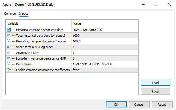
Running it on a daily S&P 500 chart with script parameters depicted above produces the following output:
 Aparch model parameters
    Name      Value     Pvalue
   omega     0.0457     0.0003
alpha[1]     0.0904     0.0000
gamma[1]     0.9997     0.0000
 beta[1]     0.8968     0.0000
   delta     0.7491     0.0000
The script is attached to this article, enabling readers to reproduce the results. Here, delta is estimated directly from the data rather than assumed. The asymmetry coefficient gamma shifts the scaling factor applied to negative versus positive shocks before exponentiation—providing a continuous slope adjustment rather than applying a distinct piecewise penalty on negative returns as seen in GJR-GARCH.
However, care must be taken when interpreting the resulting statistical output: when an estimated parameter like gamma lies near the edge of its admissible parameter space, standard asymptotic inference breaks down. In these boundary or near-boundary cases, reported standard errors and p-values can become unreliable, requiring cautious interpretation. Users of previous library iterations will notice that script code no longer requires an explicit switch to select the SLSQP solver, even though it remains in use. This is due to optimizer updates that have yielded modest efficiency gains, detailed in the next section.
SLSQP Solver Updates
In short, the most significant change is the removal of the ALGLIB solver alongside a rewritten, faster SLSQP solver. These changes have had a minimal impact on the volatility library's interface. The primary modification is to the HARX class, where fit() methods gain an additional function parameter: display_log_info. This boolean flag allows users to toggle optimizer log output for each iteration. Note that enabling this feature incurs a performance cost.
//--- Fit a model to data using SLSQP optimizer
ArchModelResult   fit(double tol = 1e-8,uint maxits = 100,ENUM_COVAR_TYPE cov_type = COVAR_ROBUST, long first = 0, long last = -1, bool display_log_info = false);

//+------------------------------------------------------------------+
//| Fit model using numerical optimization                           |
//| Orchestrates the optimization lifecycle by concatenating param   |
//| segments, stacking dynamic boundaries, and passing everything    |
//| into the SLSQP solver engine to extract optimal coefficients.    |
//+------------------------------------------------------------------+
ArchModelResult   fit(vector& startingvalues, vector& backcast, double tol = 1e-8, uint maxits = 100, ENUM_COVAR_TYPE cov_type = COVAR_ROBUST, long first = 0, long last = -1, bool display_log_info = false);
The ArchModelResult structure now also includes a member representing the result of the optimization procedure. This should make it easier to check if the solver converged correctly. Successful convergence should yield a return code with a value of zero.
//+------------------------------------------------------------------+
//| Arch model result struct                                         |
//| Inherits base properties from ArchModelFixedResult to add        |
//| statistical inference methods and parameter covariance parsing.  |
//+------------------------------------------------------------------+
struct ArchModelResult: public ArchModelFixedResult
  {
public:
   int               solver_return_code;     // Return code from the optimizer
   long              fit_indices[2];         // [0] = Start index, [1] = Stop index mapping the target data slice
   matrix            param_cov;              // Calculated parameter Variance-Covariance matrix
   double            r2;                     // Unadjusted Coefficient of Determination (R-squared)
   ENUM_COVAR_TYPE   cov_type;               // Strategy flag applied during variance calculations (Standard vs Robust)
The bulk of the refactoring was applied to the slsqp.mqh header for a cleaner implementation. The CSlsqp class retains its previous interface, with only a few deprecations and additions. The most significant change involves the convergence criteria: while the previous implementation allowed users to configure several convergence settings, the new version enforces only two—a tolerance threshold and a maximum iteration count. By default, the maximum number of iterations is set to 100 and the convergence threshold to 1e-8. This streamlines the interface and deprecates setter methods that previously specified alternative convergence criteria.
// Sets precision/accuracy targets for optimization subproblems
void              SetAcc(double acc_)
  {
   m_S.acc = acc_;
  }
// Sets the upper limit on the allowed number of function evaluation cycles
void              SetMaxEval(int maxeval)
  {
   m_S.itermax = fabs(maxeval);
  }
Configuring constraints and bounds remains unchanged. The CSlsqp class's Minimize() method also gets the display_log_info parameter.
// Main processing pipeline wrapper driving mathematical optimization mechanics over target parameters
OptimizeResult    Minimize(CFunctor &fungrad, bool display_log_info = false)
  {
   vector x0 = fungrad.initial_params(); // Query starting guess parameters from user optimization configuration class
   int n = (int)x0.Size();
   m_n = n;
   vector x_data = x0;
//---
   vector low = fungrad.lower_bounds();
   vector up = fungrad.upper_bounds();
// Dimension checking to ensure shape match constraints for boundary conditions are satisfied
   if((low.Size()&&low.Size()!=ulong(n)) || (up.Size()&&up.Size()!=ulong(n)))
     {
      Print(__FUNCTION__,": All vector inputs should be the same size if not empty");
      return OptimizeResult();
     }

// Verify bounds ordering logic
   for(int i  = 0; i<n; ++i)
      if(low[i]>up[i])
        {
         Print(__FUNCTION__ ": Invalid boundary constraints");
         return OptimizeResult();
        }

   m_obj = GetPointer(fungrad);
   m_meq = slsqp_count_constraints(ArraySize(m_eq_constraints),m_eq_constraints);
   m_m = m_meq + slsqp_count_constraints(ArraySize(m_ineq_constraints),m_ineq_constraints);

   m_S.mode = 0;
   m_S.n = m_n;
   m_S.m = m_m;
   m_S.meq = m_meq;

   int m = m_m;
   double funx = 0.0;

   double gradx[];
   ArrayResize(gradx, n);
   double C[];
   ArrayResize(C, MathMax(m*n,1));
   double d[];
   ArrayResize(d, MathMax(m,1));
   double mult[];
   ArrayResize(mult, m + 2*n + 2);

   ArrayInitialize(mult, 0.0);
   double xlw[];
   ArrayResize(xlw, n+1);
   double xuw[];
   ArrayResize(xuw, n+1);
   for(int i = 0; i < n; i++)
     {
      xlw[i] = low[i];
      xuw[i] = up[i];
     }

   int bufsize = SLSQP_BufferSize(m_n, m_m, m_meq);
   double buffer[];
   ArrayResize(buffer, bufsize);
   ArrayInitialize(buffer, 0.0);
   int indices[];
   ArrayResize(indices, m + 2*n + 2 + 16);

   double sol[];
   ArrayResize(sol, n+1);
   for(int i = 0; i < n; i++)
      sol[i] = x0[i];

   evaluate(sol, funx, gradx, d, C, true);

   int iter = 0;
   int prev_iter = -1;
   int max_driver_loops = 50*(m_S.itermax + 10);
   vector grad_v(n);
   vector fvector(1);
//---
   if(display_log_info)
      PrintFormat("%5s %5s %16s %16s","NIT", "FC", "OBJFUN", "GNORM");
//---
   while(!IsStopped())
     {
      iter++;
      if(iter > max_driver_loops)
        {
         if(display_log_info && m_S.iter != prev_iter)
           {
            vector gnorm;
            gnorm.Assign(gradx);
            PrintFormat("%5i %5i % 16.6E % 16.6E", m_S.iter, iter, funx, gnorm.Norm(VECTOR_NORM_P));
           }
         m_S.mode = 9;
         break;
        }
      SLSQPBody(m_S, funx, gradx, C, d, sol, mult, xlw, xuw, buffer, indices);
      if(m_S.mode == 1)
        {
         evaluate(sol, funx, gradx, d, C, false);
        }
      else
         if(m_S.mode == -1)
           {
            evaluate(sol, funx, gradx, d, C, true);
           }
         else
           {
            if(display_log_info && m_S.iter != prev_iter)
              {
               vector gnorm;
               gnorm.Assign(gradx);
               PrintFormat("%5i %5i % 16.6E % 16.6E", m_S.iter, iter, funx, gnorm.Norm(VECTOR_NORM_P));
              }
            break;
           }

      if(display_log_info && m_S.iter != prev_iter)
        {
         vector gnorm;
         gnorm.Assign(gradx);
         PrintFormat("%5i %5i % 16.6E % 16.6E", m_S.iter, iter, funx, gnorm.Norm(VECTOR_NORM_P));
        }

      prev_iter = m_S.iter;
     }
//---
   Copy(x0,sol,n);
   Copy(grad_v,gradx,n);
   fvector[0] = funx;
   if(IsStopped())
      m_S.mode = -2;
//---
   if(display_log_info)
     {
      Print("Exit mode: ", GetExitMode(m_S.mode));
      Print("            Current function value:", funx);
      Print("            Iterations:", m_S.iter);
      Print("            Function evaluations:", m_obj.nfev());
      Print("            Gradient evaluations:", m_obj.ngev());
     }
// Pack successful calculations tracking profiles into result layout container blocks
   return OptimizeResult(int(m_S.mode),m_S.iter,iter,x0,fvector,grad_v);
  }
This updated implementation brings the library into even closer parity with the original Python ARCH package, as demonstrated by the validation tests in the next section.
Nesting Existing Models with APARCH
The flexible nature of the APARCH framework enables it to nest other models already implemented in this library. Its implementation can be partially validated by constraining APARCH's delta and gamma parameters to specific values to reproduce close approximations of the conditional volatility series generated by standard GARCH and GJR-GARCH configurations.
//+------------------------------------------------------------------+
//| Script program start function                                    |
//+------------------------------------------------------------------+
void OnStart()
  {
//---
   vector prices;
//--- Pull close prices directly into an array using native vector operations
   if(!prices.CopyRates(NULL,PERIOD_CURRENT, COPY_RATES_CLOSE,0, HistoryLen))
     {
      Print(" failed to get close prices for ", _Symbol, ". Error ", GetLastError());
      return;
     }

//--- Map closing prices to logarithmic space
   prices = log(prices);

//--- Compute log returns: r_t = ln(P_t) - ln(P_{t-1})
   vector returns = np::diff(prices) * ScaleFactor;
//---
   ENUM_VOLATILITY_MODEL vol_models[2] = {VOL_GARCH,VOL_GJR_GARCH};// --- The volatility processes to reproduce
   vector Xs;                                                                // --- x-axis values (time index)
   vector Ys[2];                                                             // --- containers for conditional volatility series of each model
   string Ylabels[2];                                                        // --- line plot names
//--- Test Aparch vs Other models
   for(uint i = 0; i<vol_models.Size(); ++i)
      if(compare_models(vol_models[i],returns,Xs,Ys,Ylabels))
         np::plotxys(Xs,Ys,Ylabels,"Conditional Volatility Series Comparison","Time Index","Conditional Volatility",false,0,0,30,40,750,500,true,2,1,15);
  }
The APARCH_NestingTest.mq5 program is an MQL5 script designed to demonstrate the nesting equivalence of restricted ARCH-family models within the APARCH architecture. The script sequentially evaluates two classical volatility models—standard GARCH(1,1) and asymmetric GJR-GARCH(1,1,1)—against their APARCH equivalents. In the helper function compare_models(), an APARCH process is constructed with parameters constrained to replicate the candidate process, such as setting the power parameter to 2.0 alongside specific asymmetry specifications. The function also quantifies the numerical differences between the conditional volatility series by calculating the mean squared difference and mean absolute difference for display in the terminal's Experts tab.
//+----------------------------------------------------------------------------------+
//|Takes a model either GJR,GARCH or TARCH and compares it to equivalent APARCH model|
//+----------------------------------------------------------------------------------+
bool compare_models(ENUM_VOLATILITY_MODEL vol_model, vector& returns_data,vector& X, vector& Ys[], string& YPlotNames[])
  {
   YPlotNames[0] = "APARCH";
//---
   ulong p,o,q;
   double pwr;
//--- Initialize core specification fields mapping onto the aparch container
   ArchParameters spec;
//--- Apply the scaling factor (multiplying by 100 scales returns to percentage form)
   spec.observations = returns_data;
//---
   switch(vol_model)
     {
      case VOL_GARCH:
         p = 1;
         q = 1;
         o = 0;
         pwr = 2.0;
         YPlotNames[1] = "GARCH";
         break;
      case VOL_GJR_GARCH:
         p = 1;
         q = 1;
         o = 1;
         pwr = 2.0;
         YPlotNames[1] = "GJR-GARCH";
         break;
      default:
         Print("Invalid volatility model input");
         return false;
     }
//---
   spec.vol_model_type = VOL_APARCH;
   spec.garch_p = p;
   spec.garch_o = o;
   spec.garch_q = q;
   spec.aparch_delta = pwr;
//--- Instantiate the zero mean container wrapper
   ZeroMean aparch_model;
//--- Pass structural parameters down into the optimization initialization routine
   if(!aparch_model.initialize(spec))
      return false;
//--- Trigger the non-linear execution optimizer loop (SLSQP engine solver)
   ArchModelResult aparch_params = aparch_model.fit();
//--- Verify that the resulting parameters array size matches the model criteria configurations
   if(aparch_params.solver_return_code)
     {
      Print("Convergence failed ", Optimization return code ", aparch_params.solver_return_code);
      return false;
     }
//---
   Ys[0] = aparch_params.conditional_volatility;
//---
   spec.vol_model_type = vol_model;
   spec.garch_p = p;
   spec.garch_o = o;
   spec.garch_q = q;
   spec.vol_power = pwr;
//---
   ZeroMean other_model;
//--- Pass structural parameters down into the optimization initialization routine
   if(!other_model.initialize(spec))
      return false;
//--- Trigger the non-linear execution optimizer loop (SLSQP engine solver)
   ArchModelResult other_params = other_model.fit();
//--- Verify convergence
   if(other_params.solver_return_code)
     {
      Print("Convergence failed. Optimization return code ", other_params.solver_return_code);
      return false;
     }
//--- Get the conditional volatility series
   Ys[1] = other_params.conditional_volatility;
   vector difference = Ys[0] - Ys[1];
//---
   PrintFormat("%s vs %s", YPlotNames[0], YPlotNames[1]);
   PrintFormat("Mean squared difference %.8f", MathPow(difference, 2.0).Mean());
   PrintFormat("Mean absolute difference %.8f", MathAbs(difference).Mean());
//--- Set the x-axis values
   X = np::arange(Ys[1].Size());
//---
   return true;
  }
The script fits both the explicit classical model and its parameter-restricted APARCH counterpart to the same return series using a zero-mean assumption, extracts their fitted conditional volatility paths, and renders a two-line comparative overlay plot for analysis. Running the script with the default parameters on the EURUSD daily chart produces the plots observed below.
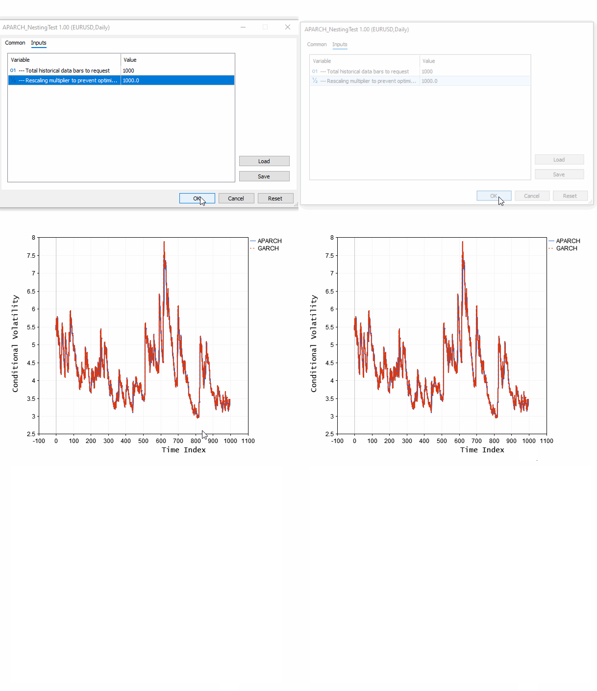
Small numerical differences between the two series are expected, as CGarchProcess precomputes its power-transformed residuals directly while CAparchProcess derives the equivalent quantity through a shift term held at zero; the two paths should agree within floating-point precision rather than match identically. A large or growing divergence would indicate an implementation error in the new recursion rather than legitimate model disagreement, given that the classes are constrained to coincide. This is shown by the script's output to the terminal's logs, displayed below.
APARCH vs GARCH
Mean squared difference 0.00000000
Mean absolute difference 0.00005247
APARCH vs GJR-GARCH
Mean squared difference 0.00000002
Mean absolute difference 0.00006933
The APARCH Volatility Indicator
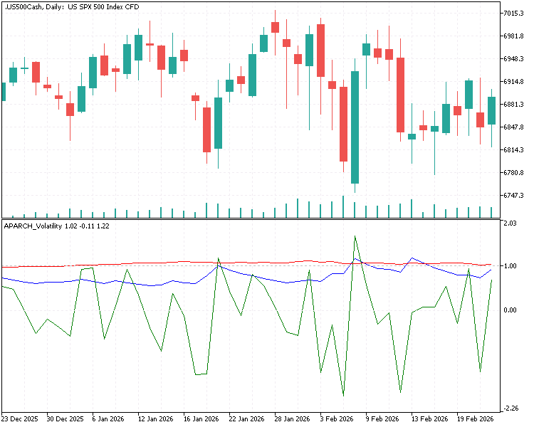
The APARCH volatility indicator mirrors the EGARCH volatility indicator introduced earlier in this series: it fits an APARCH model over a rolling window of historical returns and plots the resulting conditional volatility, standardized residuals, and delta parameter. The indicator lets users observe not just how volatility is moving, but also whether the shape of the volatility response itself—its effective power and asymmetry—is drifting over time. A steady decline in delta alongside rising volatility, for instance, suggests that the market's response to shocks is becoming closer to linear than quadratic—information a fixed-power model-based indicator cannot provide. The indicator is shown below. The blue line represents conditional volatility, the green line depicts standardized residuals, and the red line tracks the delta parameter.
Benchmarking APARCH
In this section, we present the APARCH_Benchmark.mq5 script to evaluate and compare the statistical performance and forecasting capabilities of various ARCH-family volatility models against the APARCH model. Again, the goal is not to affirm the superiority of APARCH but to demonstrate its capabilities.
//--- Script Inputs
input int      InpHoldoutSize   = 100;         // Forecast horizon
input int      InpInSampleSize  = 1000;        // In-Sample Training Bar Count
input ENUM_TIMEFRAMES InpTimeframe = PERIOD_D1;// Execution Timeframe
input double    InpScaleFactor  = 100.0;       // Scaling multiplier
input ENUM_FORECAST_METHOD InpForeCastMethod = FORECAST_ANALYTIC; // Forecasting method

// Struct to store final benchmarking metrics for each model
struct ModelPerformance
  {
   string   model_name;
   double   aic;
   double   bic;
   double   oos_mse;
   double   oos_mae;
   double   log_like;
  };

//+------------------------------------------------------------------+
//| Script program start function                                    |
//+------------------------------------------------------------------+
void OnStart()
  {
   if(InpHoldoutSize<=0 || InpInSampleSize<50)
    {
     Alert("Invalid input parameters for InpHoldoutSize and/or InpInSampleSize\nBoth must be >0 and >=50 respectively.");
     return;
    }
   Print("==========================================================");
   Print(" Starting Volatility Model Evaluation: APARCH vs. Competitors");
   Print("==========================================================");

   // Prepare Returns Data
   ulong total_needed = (ulong)(InpInSampleSize + InpHoldoutSize + 1);
   vector close_prices;

   if(!close_prices.CopyRates(_Symbol, InpTimeframe, COPY_RATES_CLOSE, 0, (uint)total_needed))
     {
      Print("Error: Failed to fetch price data.");
      return;
     }

   // Compute Log Returns: r_t = ln(P_t / P_{t-1}) * scalefactor
   ulong n_returns = close_prices.Size() - 1;
   vector returns(n_returns);
   for(ulong i = 0; i < n_returns; ++i)
     {
      returns[i] = MathLog(close_prices[i + 1] / close_prices[i]) * InpScaleFactor;
     }

   // Split into In-Sample and Out-of-Sample arrays
   ulong in_sample_len = n_returns - (ulong)InpHoldoutSize;
   vector in_sample_returns = np::sliceVector(returns, 0, (long)in_sample_len);
   vector oos_returns       = np::sliceVector(returns, (long)in_sample_len, (long)n_returns);

   // Realized variance benchmark for OOS (using squared returns as proxy)
   vector oos_realized_variance = MathPow(oos_returns, 2.0);

   // Define Volatility Models to Compare
   ENUM_VOLATILITY_MODEL models[] =
     {
      VOL_GARCH,
      VOL_GJR_GARCH,
      VOL_EGARCH,
      VOL_TARCH,
      VOL_APARCH
     };

   string model_names[] =
     {
      "GARCH(1,1)",
      "GJR-GARCH(1,1,1)",
      "EGARCH(1,1,1)",
      "TARCH(1,1,1)",
      "APARCH(1,1,1)"
     };

   uint num_models = ArraySize(models);
   ModelPerformance results[];
   ArrayResize(results, num_models);

   // Loop Through and Fit Each Model
   for(uint i = 0; i < num_models; ++i)
     {
      PrintFormat("\n--- Fitting Model [%d/%d]: %s ---", i + 1, num_models, model_names[i]);

      // Populate base ARCH parameters structure
      ArchParameters params;
      params.observations       = in_sample_returns;
      params.mean_model_type    = MEAN_CONSTANT;
      params.vol_model_type     = models[i];
      params.dist_type          = DIST_NORMAL;
      params.garch_p            = 1;
      params.garch_o            = 1; // Asymmetry term enabled where applicable
      params.garch_q            = 1;

      // Special APARCH specific defaults if selected
      if(models[i] == VOL_APARCH)
        {
         params.aparch_delta       = EMPTY_VALUE; // Jointly estimate dynamic power parameter
         params.aparch_common_asym = false;
        }

      // Construct model instance (using CConstantMean model wrapper)
      ConstantMean model;
      if(!model.initialize(params))
        {
         PrintFormat("Failed to initialize model: %s", model_names[i]);
         continue;
        }

      // Optimize parameters over In-Sample dataset
      ArchModelResult fit_result = model.fit();

      if(fit_result.solver_return_code != 0)
        {
         PrintFormat("Warning: Solver ended with code %d for model %s", fit_result.solver_return_code, model_names[i]);
        }

      // Record In-Sample Information Criteria
      results[i].model_name = model_names[i];
      results[i].log_like   = fit_result.loglikelihood;
      results[i].aic        = fit_result.aic();
      results[i].bic        = fit_result.bic();

      // Evaluate Out-of-Sample (OOS) Volatility Forecasts
      matrix dummy_x[];
      vector fitted_params = model.get_params();

      // Perform multi-step analytical forecast across the holdout period
      ArchForecast fcast = model.forecast(fitted_params, dummy_x, (ulong)InpHoldoutSize, -1, InpForeCastMethod);

      if(fcast.variance.Rows() > 0)
        {
         // Extract 1-step to H-step variance forecast vector
         vector pred_variance = fcast.variance.Row(fcast.variance.Rows() - 1);

         // Calculate Forecast Error Metrics (Predicted Variance vs Realized Proxy)
         vector errors = oos_realized_variance - pred_variance;

         results[i].oos_mse = MathPow(errors, 2.0).Mean();
         results[i].oos_mae = MathAbs(errors).Mean();
        }
      else
        {
         results[i].oos_mse = DBL_MAX;
         results[i].oos_mae = DBL_MAX;
        }
     }

   // Print Comparison Summary Report Table
   Print("\n=========================================================================");
   Print("                        MODEL COMPARISON RESULTS                         ");
   Print("=========================================================================");
   PrintFormat("%-15s | %-12s | %-12s | %-12s | %-12s", "Model", "AIC", "BIC", "OOS MSE", "OOS MAE");
   Print("-------------------------------------------------------------------------");

   int best_aic_idx = 0;
   int best_mse_idx = 0;

   for(uint i = 0; i < num_models; ++i)
     {
      PrintFormat("%-15s | %-12.4f | %-12.4f | %-12.6f | %-12.6f",
                  results[i].model_name,
                  results[i].aic,
                  results[i].bic,
                  results[i].oos_mse,
                  results[i].oos_mae);

      if(results[i].aic < results[best_aic_idx].aic) best_aic_idx = (int)i;
      if(results[i].oos_mse < results[best_mse_idx].oos_mse) best_mse_idx = (int)i;
     }

   Print("-------------------------------------------------------------------------");
   PrintFormat("Optimal In-Sample Fit (Lowest AIC): %s", results[best_aic_idx].model_name);
   PrintFormat("Optimal Out-of-Sample Robustness (Lowest MSE): %s", results[best_mse_idx].model_name);
   Print("=========================================================================");
  }
The program begins by retrieving historical data for a user-defined timeframe and calculating percentage log returns. The returns are then partitioned into two distinct segments: an in-sample training dataset used for parameter estimation and an out-of-sample holdout dataset used to test future predictive capabilities. It constructs and fits five volatility specifications—standard GARCH, GJR-GARCH, EGARCH, TARCH, and APARCH—to the in-sample data. For each model, it records the optimized log-likelihood alongside the Akaike Information Criterion (AIC) and Bayesian Information Criterion (BIC). Finally, the script leverages the fitted models to generate multi-step variance forecasts across the holdout horizon, computing the Mean Squared Error (MSE) and Mean Absolute Error (MAE) by comparing predicted variances against out-of-sample realized variance proxies before displaying a final comparison matrix in the terminal's Experts tab.
Interpreting the benchmarking results requires looking at both the in-sample model fit and the out-of-sample forecasting precision. The in-sample information criteria, AIC and BIC, evaluate how efficiently a model captures the underlying variance process while penalizing for unnecessary parameter complexity; lower AIC and BIC values highlight the model that achieves the best statistical trade-off. The out-of-sample metrics, MSE and MAE, estimate predictive performance.
Despite its utility, this benchmarking methodology carries notable limitations that must be kept in mind during practical application. Relying on squared returns as a proxy for out-of-sample realized variance introduces considerable noise, as raw squared returns are highly inefficient estimates of true daily variance. Additionally, the evaluation depends heavily on the chosen sample split; a single fixed out-of-sample period may capture an atypical market regime, such as a sudden spike or prolonged quiet phase, which can artificially favor or penalize certain model structures. Furthermore, multi-step analytical forecasts for non-linear models like EGARCH or APARCH can suffer from Jensen's inequality bias over longer horizons, indicating that static multi-step projections may diverge from actual path-dependent variance unless re-fitted dynamically using rolling 1-step-ahead forecast schemes.
//--- Script Inputs
input int      InpHoldoutSize   = 100;         // Forecast horizon
input int      InpInSampleSize  = 1000;        // In-Sample Training Bar Count
input ENUM_TIMEFRAMES InpTimeframe = PERIOD_H1;// Execution Timeframe
input double    InpScaleFactor  = 1000.0;      // Scaling multiplier
input ENUM_FORECAST_METHOD InpForeCastMethod = FORECAST_SIMULATION; // Forecasting method
The script was applied to the AUDUSD hourly chart with the most recent bar dated 2026.09.25, using the parameters above, which produced the output shown below.
=========================================================================
                        MODEL COMPARISON RESULTS
=========================================================================
Model           | AIC          | BIC          | OOS MSE      | OOS MAE
-------------------------------------------------------------------------
GARCH(1,1)      | 2363.9283    | 2383.5593    | 2.437198     | 1.049349
GJR-GARCH(1,1,1) | 2360.6995    | 2385.2383    | 2.561327     | 1.191519
EGARCH(1,1,1)   | 2355.1415    | 2379.6802    | 2.332528     | 0.827687
TARCH(1,1,1)    | 2339.6755    | 2364.2143    | 2.339047     | 0.895008
APARCH(1,1,1)   | 2331.6289    | 2361.0754    | 2.329904     | 0.877488
-------------------------------------------------------------------------
Optimal In-Sample Fit (Lowest AIC): APARCH(1,1,1)
Optimal Out-of-Sample Robustness (Lowest MSE): APARCH(1,1,1)
=========================================================================
In spite of APARCH's showing here, it should be noted that a single set of results does not prove the overall superiority of APARCH.
Conclusion
This article extends the conditional volatility library with the Asymmetric Power ARCH (APARCH) model. The exponent applied to shocks and the shape of the asymmetric response can now be estimated directly from the data, rather than being fixed in advance by the analyst. With the addition of the CAparchProcess class, the library implements the core APARCH model specification. Furthermore, the nesting relationship demonstrated earlier shows that this new class correctly reduces to standard GARCH and GJR-GARCH processes when appropriately constrained.
The APARCH_Volatility indicator introduced here offers a practical demonstration of how delta varies over time alongside conditional volatility, providing a clear picture of the structural limitations imposed by simpler, fixed-power models. The source code for all programs referenced in this text is attached below and is also available on MQL5 Algo Forge.
| MQL5/Include/aparch/np.mqh. | Header file of various vector and matrix utility functions |
| MQL5/Include/aparch/Arch | Folder of header files for the conditional volatility modeling library, including the new CAparchProcess class and aparch_recursion() function |
| MQL5/Scripts/aparch/APARCH_Demo.mq5 | This script demonstrates fitting an APARCH model to a dataset |
| MQL5/Scripts/aparch/APARCH_NestingTest.mq5 | This script validates the APARCH implementation against the existing GARCH classes under nesting restrictions |
| MQL5/Scripts/aparch/APARCH_Benchmark.mq5 | A script used to compare the model properties and predictive performance of APARCH against select ARCH frameworks |
| MQL5/Indicators/aparch/APARCH_Volatility.mq5 | This is the APARCH volatility indicator's source code. |
Warning: All rights to these materials are reserved by MetaQuotes Ltd. Copying or reprinting of these materials in whole or in part is prohibited.
This article was written by a user of the site and reflects their personal views. MetaQuotes Ltd is not responsible for the accuracy of the information presented, nor for any consequences resulting from the use of the solutions, strategies or recommendations described.
 Features of Custom Indicators Creation
 Trade Duration vs Profitability Scatter Plot Indicator in MQL5
 Features of Experts Advisors
 Neural Networks in Trading: Robust Trading Signals in Any Market Regime (ST-Expert)

- Free trading apps
- Over 8,000 signals for copying
- Economic news for exploring financial markets
You agree to website policy and terms of use