Detecting and Classifying Fractal Patterns Using Machine Learning

Introduction

In the first article, we have examined in detail the fundamental aspects of the multifractal market theory. We noted that price charts are capable of forming certain repeating structures under the influence of external information that organizes them. Market participants create a complex dynamic system that has memory elements that take the form of certain market symmetries (patterns). These patterns may evolve over time or may repeat. Due to the self-similarity of fractal market structures, patterns can be expressed across different time scales.

This article presents an original approach to identifying and classifying fractal patterns. The analysis will be conducted in Python, with the ability to export final models to the MetaTrader 5 terminal in ONNX format.

Before you begin, make sure you have installed all the required packages and modules. Some of the imported modules are included in the attachment below.

import pandas as pd
import math
from datetime import datetime
from catboost import CatBoostClassifier
from sklearn.model_selection import train_test_split
from bots.botlibs.labeling_lib import *
from bots.botlibs.tester_lib import test_model
from bots.botlibs.export_lib import export_model_to_ONNX

Implementation of the fractal pattern search function

In this article, I propose a simple approach to finding symmetrical multifractal market structures through correlation. We can explore both fractal and multifractal patterns, which are scale invariant, that is, they have different sizes. To do this, it is necessary to implement a search for patterns through correlation on different time scales, which will be specified in the settings. Below is a function that calculates correlation in a sliding window taking into account the variable length of patterns.

@njit
def calculate_symmetric_correlation_dynamic(data, min_window_size, max_window_size):
    n = len(data)
    min_w = max(2, min_window_size)
    max_w = max(min_w, max_window_size)
    num_correlations = max(0, n - min_w + 1)

    if num_correlations == 0:
        return np.zeros(0, dtype=np.float64), np.zeros(0, dtype=np.int64)

    correlations = np.zeros(num_correlations, dtype=np.float64)
    best_window_sizes = np.full(num_correlations, -1, dtype=np.int64)

    for i in range(num_correlations):
        max_abs_corr_for_i = -1.0
        best_corr_for_i = 0.0
        current_best_w = -1
        current_max_w = min(max_w, n - i)
        start_w = min_w
        if start_w % 2 != 0:
            start_w += 1

        for w in range(start_w, current_max_w + 1, 2):
            if w < 2 or i + w > n:
                continue
            half_window = w // 2
            window = data[i : i + w]
            first_half = window[:half_window]
            second_half = (window[half_window:] * -1)[::-1]
            
            std1 = np.std(first_half)
            std2 = np.std(second_half)

            if std1 > 1e-9 and std2 > 1e-9:
                mean1 = np.mean(first_half)
                mean2 = np.mean(second_half)
                cov = np.mean((first_half - mean1) * (second_half - mean2))
                corr = cov / (std1 * std2)
                if  abs(corr) > max_abs_corr_for_i:
                    max_abs_corr_for_i = abs(corr)
                    best_corr_for_i =corr
                    current_best_w = w
        
        correlations[i] = best_corr_for_i
        best_window_sizes[i] = current_best_w
        
    return correlations, best_window_sizes

To speed up a loop with similar calculations (loops are slow in Python), the @njit decorator is used, which speeds up calculations using the Numba package. 

The function accepts as input a data frame with closing prices, as well as the minimum and maximum "window" sizes for patterns. For example, we want to calculate the correlation for patterns whose length is from 100 to 200 bars. Then we set the appropriate settings, after which the correlation between its left and mirror-inverted right parts is checked for each new reference point and for each given pattern length. The inversion of the right half is highlighted in yellow. This is very important because we are looking for symmetry in the data.

The values of the best absolute correlations for each starting point are written to the correlations[] array. The window size (pattern length) corresponding to the best correlation is written to another array best_window_sizes[]. Thus, the function returns the maximum correlation values and the corresponding pattern for each starting point.

Visual check of the found patterns

Once all the patterns have been calculated, we can visually assess the correctness of our algorithm. For this purpose, I propose another function that will display the top best patterns found by the highest absolute Pearson correlation coefficient.

def plot_best_n_patterns(data, min_window_size, max_window_size, n_best):
    # 1. Calculate correlations and best window sizes
    corrs, window_sizes = calculate_symmetric_correlation_dynamic(data, min_window_size, max_window_size)

    # 2. Find N best patterns
    # Assuming -1 in window_sizes means invalid/not found by the calculation logic
    valid_calc_mask = window_sizes != -1 
    
    if not np.any(valid_calc_mask):
        print("No suitable patterns found (all window sizes were marked as -1 by calculation).")
        return
        
    filtered_corrs = corrs[valid_calc_mask]
    filtered_window_sizes = window_sizes[valid_calc_mask]
    
    original_indices_all = np.arange(len(corrs)) 
    filtered_start_indices = original_indices_all[valid_calc_mask]

    if len(filtered_corrs) == 0: 
        print("No suitable patterns found after filtering out -1 window_sizes.")
        return

    # Sort by absolute correlation value in descending order
    sorted_indices_of_filtered = np.argsort(np.abs(filtered_corrs))[::-1]
    
    # Determine how many of the top patterns to consider
    num_to_consider = min(n_best, len(sorted_indices_of_filtered))

    if num_to_consider == 0:
        print("No patterns to plot (either n_best is too small, or no patterns passed the initial filter).")
        return

    # Pre-filter these top candidates to find those actually plottable (even window size >= 2)
    patterns_to_plot_details = []
    for i in range(num_to_consider):
        idx_in_filtered_arrays = sorted_indices_of_filtered[i] # Index within the already filtered (by valid_calc_mask) arrays
        
        w_best_candidate = filtered_window_sizes[idx_in_filtered_arrays]
        actual_data_start_index = filtered_start_indices[idx_in_filtered_arrays]
        correlation_value = filtered_corrs[idx_in_filtered_arrays]
        
        # Check if the window size is valid for plotting (even and sufficiently large)
        if w_best_candidate >= 2 and w_best_candidate % 2 == 0 : 
            patterns_to_plot_details.append({
                "original_rank_in_consider_list": i, # Rank among the num_to_consider items
                "data_start_index": actual_data_start_index,
                "correlation": correlation_value,
                "window_size": int(w_best_candidate) # Ensure it's int
            })
        else:
            print(f"Info: Top candidate (originally rank {i+1} among considered, "
                  f"Start Index: {actual_data_start_index}) "
                  f"skipped due to invalid window size for plotting: {w_best_candidate} (must be even and >= 2).")


    num_actually_plotted = len(patterns_to_plot_details)

    fig, ax = plt.subplots(1, 1, figsize=(10, 5)) # Single axes for combined plot
    title_fontsize = 12
    label_fontsize = 10
    legend_fontsize = 8
    tick_labelsize = 9

    if num_actually_plotted == 0:
        # This message is shown if, out of the top 'num_to_consider' patterns, none had a valid window size for plotting.
        print("No patterns with valid window sizes (even, >=2) found among the top candidates to display on the chart.")
        ax.text(0.5, 0.5, "No valid patterns to display on the chart.",
                horizontalalignment='center', verticalalignment='center',
                transform=ax.transAxes, fontsize=title_fontsize, color='red')
        ax.set_xticks([])
        ax.set_yticks([])
        fig.suptitle(f"Symmetric Patterns Overlaid", fontsize=title_fontsize) # Generic title
    else:
        # Generate distinct colors for each pattern that will actually be plotted
        plot_colors = plt.cm.viridis(np.linspace(0, 1, num_actually_plotted))

        for plot_idx, pattern_info in enumerate(patterns_to_plot_details):
            actual_data_start_index = pattern_info["data_start_index"]
            correlation_value = pattern_info["correlation"]
            w_best = pattern_info["window_size"]
            
            half_window = w_best // 2
            
            # Ensure indices are within data bounds
            if actual_data_start_index + w_best > len(data):
                print(f"Warning: Pattern P{plot_idx+1} (Idx:{actual_data_start_index}, W:{w_best}) extends beyond data length {len(data)}. Skipping.")
                continue

            left_part_data = data[actual_data_start_index : actual_data_start_index + half_window]
            right_part_data = data[actual_data_start_index + half_window : actual_data_start_index + w_best]
            
            x_indices = np.arange(w_best) # X-axis relative to pattern start
            current_color = plot_colors[plot_idx]

            # Plot left part
            ax.plot(x_indices[:half_window], left_part_data, 
                    color=current_color, linestyle='-', 
                    label=f"P{plot_idx+1} (Idx:{actual_data_start_index}, W:{w_best}, C:{correlation_value:.2f})")
            
            # Plot right part
            ax.plot(x_indices[half_window:], right_part_data, 
                    color=current_color, linestyle='--') 
            
            # Add a vertical line to mark the split point for this pattern
            ax.axvline(x=half_window - 0.5, color=current_color, linestyle=':', linewidth=1, alpha=0.6)

        ax.set_xlabel("Index within Pattern Window", fontsize=label_fontsize)
        ax.set_ylabel("Data Value", fontsize=label_fontsize)
        ax.tick_params(axis='both', which='major', labelsize=tick_labelsize)
        ax.grid(True)
        
        ax.legend(fontsize=legend_fontsize, loc='best')
        # Add a text note to explain line styles
        fig.text(0.99, 0.01, 'Solid: Left Part, Dashed: Right Part (Original)', 
                 horizontalalignment='right', verticalalignment='bottom', 
                 fontsize=legend_fontsize - 1, color='dimgray', transform=fig.transFigure)

        fig.suptitle(f"Top {num_actually_plotted} Symmetric Patterns Overlaid", fontsize=title_fontsize)

    plt.tight_layout(rect=[0, 0.03, 1, 0.96]) # Adjust rect for suptitle and fig.text
    plt.show()

This function is fairly lengthy, but most of the code handles pattern sorting and plotting. First, the patterns themselves are calculated, then they are sorted by the values of the correlation coefficient. Each pattern’s position in the price history is identified and then plotted. The result of this function is shown below.

In the first image, we see one selected pattern that has the highest absolute correlation. It resembles a certain peak, local or global, which symbolizes a trend reversal. The dotted vertical line marks the split of the series into two equal halves. The right half is sign-inverted and mirrored. After this, the correlation between the left and right sections is calculated. The charts do not show the inverted right-hand sides, but the original source series of quotes.

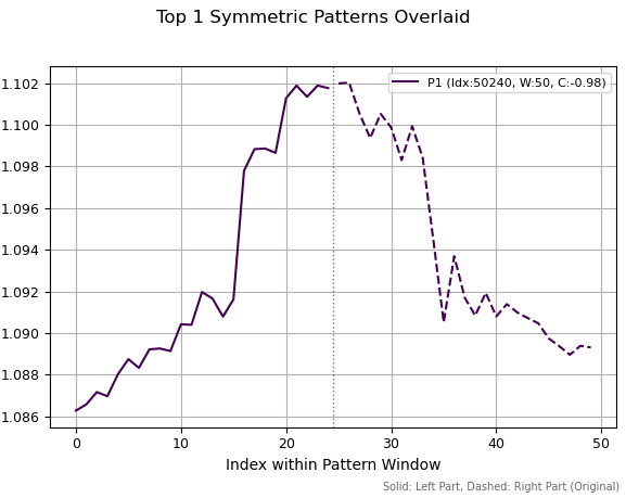
Fig. 1. The best pattern has a period of 50 and a correlation of -0.98

In the second figure, I have displayed the five best patterns with a period of 50. Of these five patterns, three resemble tops, two resemble bottoms; one of them also looks like a continuation of a bullish trend. The scale on the left displays the historical price levels these patterns correspond to.

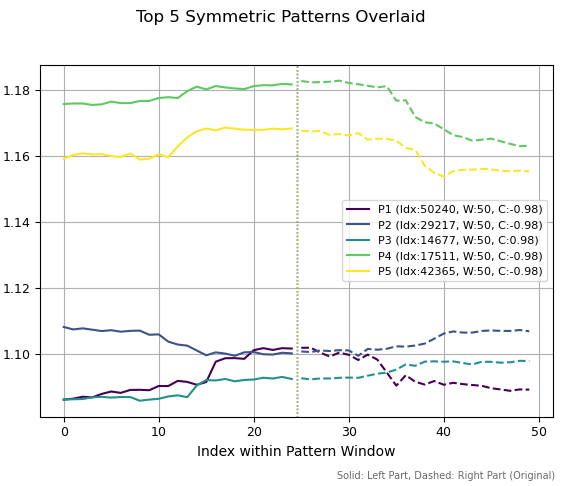
Fig. 2. Top five 50-period patterns

If we increase the pattern periods to 150 bars, completely different structures are observed. Three similar patterns were found (top). This is because a small shift in history resulted in the discovery of the same structure. The other two patterns turned out different from each other.

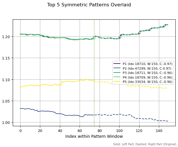
Fig. 3. Top five patterns with a period of 150

If we increase the pattern calculation window to 250, the same patterns again turned out to be among the best, but with a slight shift in history. Some reversal patterns can also be observed, as their correlations are negative.

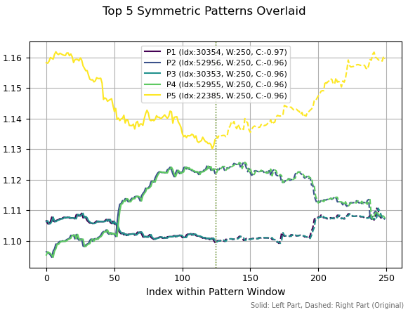
Fig. 4. Top five patterns with a period of 250

These illustrations demonstrate a wide variety of self-affine (self-similar) market structures. Theoretically, this diversity can only be limited by the length of the series under study. In this case, it is quite difficult to determine which specific pattern will have predictive potential and which will not. It would take months to study each individual structure. Machine learning can help us here, as it allows us to classify all patterns at once.

It is quite possible that searching for structures through correlation is not ideal, and other, more accurate estimation methods should be considered. But this approach is a good starting point for further research and is intuitive. Now we need to figure out how to analyze these market fractals and build a trading system based on them using machine learning.

Labeling trades based on symmetrical structures

The function of finding symmetric structures is, in a sense, a data mining function. We set clear criteria for what we are looking for in the data - self-similar fractal structures. Next, it is necessary to collect and classify the information received. But even this will not be enough, because we will have to come up with a way to label trades based on this data, which is what we will do in this section.

I propose the following method of labeling trades for subsequent classification. It is not the only possible one, but reflects the author’s understanding of how it can be implemented. I believe that further research is needed on this topic, but for now we will limit ourselves to the existing markup method.

@njit
def generate_future_outcome_labels_for_patterns(
    close_data_len,                 #  Total length of the original close_data
    correlations_at_window_start,   # Correlation array
    window_sizes_at_window_start,   # Array of window sizes
    source_close_data,              # Full close_data array
    correlation_threshold,
    min_future_horizon,             # Minimum horizon for determining the future price
    max_future_horizon,             # Maximum horizon
    markup_points                   # "Markup" for determining a significant price change
):
    labels = np.full(close_data_len, 2.0, dtype=np.float64)  # 2.0: no signal/neutral/no pattern
    num_potential_windows = len(correlations_at_window_start)

    for idx_window_start in range(num_potential_windows):
        corr_value = correlations_at_window_start[idx_window_start]
        w = window_sizes_at_window_start[idx_window_start]

        # Condition 1: The correlation should be strong enough
        if abs(corr_value) < correlation_threshold:
            continue

        # Condition 2: A valid window should be found
        if w < 2:
            continue

        # The point in time (index) when the correlation pattern is fully formed
        signal_time_idx = idx_window_start + w - 1

        if signal_time_idx >= close_data_len: # Theoretically, this should not happen
            continue
            
        # Array for storing labels for the entire pattern (both left and right parts)
        pattern_labels = []
            
        # Calculate individual marks for all points of the pattern
        for point_idx in range(idx_window_start, signal_time_idx + 1):
            # Current price for this particular point
            current_price = source_close_data[point_idx]
            
            # Define the forecast horizon
            current_horizon = min_future_horizon
            if max_future_horizon > min_future_horizon:
                current_horizon = random.randint(min_future_horizon, max_future_horizon)
            
            # Index of future price relative to the current point
            future_price_idx = point_idx + current_horizon
            
            if future_price_idx >= close_data_len:
                continue
                
            future_price = source_close_data[future_price_idx]
            
            # Define a label for the current point
            current_label = 2.0  # Neutral by default
            if future_price > current_price + markup_points:
                current_label = 0.0  # Price increased
            elif future_price < current_price - markup_points:
                current_label = 1.0  # Price fell
                
            # Add the label to the array if it is not neutral
            if current_label != 2.0:
                pattern_labels.append(current_label)
        
        # If there are no significant marks in the pattern, move on to the next pattern
        if len(pattern_labels) == 0:
            continue
            
        # Calculate the average mark for all points of the pattern
        avg_label = 0.0
        for l in pattern_labels:
            avg_label += l
        avg_label /= len(pattern_labels)
        
        # Define a common label for the entire pattern
        pattern_label = 0.0 if avg_label < 0.5 else 1.0
        
        # Assign this label to all points of the pattern
        for i in range(idx_window_start, signal_time_idx + 1):
            labels[i] = pattern_label
        
    return labels

The generate_future_outcome_labels_for_patterns() function implements the following functionality:

• The input is the original array of prices, an array of correlations, and an array of pattern lengths corresponding to the largest correlations for a particular data point. The function also accepts a minimum and maximum forecast horizon, in bars.
• Initially, all trades are marked as 2.0 (do not trade).
• The loop checks the correlation value for each point in the time series. If the correlation exceeds correlation_threshhold, then this observation undergoes additional processing, otherwise the label for this example remains 2.0.
• Then, throughout the entire length of the pattern, determined through the maximum correlation, trades are calculated based on future price changes. For each point: if the price has risen, then this is the 0 mark - buy, if the price has fallen, then this is 1 - sell. The average value is found across trades, and an average mark is assigned to each observation of the current pattern.

The philosophy behind this approach is that highly correlated structures have a "memory" of their initial conditions and exhibit some degree of regularity. This means that observations within them are better predicted, but to prevent overfitting, we put an average label on each observation. Conversely, observations within low-correlation structures are poorly predicted because they have less regularity.

As a result, we exploit the following principle: one model will determine the quality of the pattern (whether it is worth trading at the moment or not), and the other model will determine the direction of trading. Machine learning will be tasked with approximating all possible patterns and trading directions.

Next, we will need another orchestrator function, which will be called directly for labeling trades.

The final fractal pattern-based markup function

It is time to put it all together and write a trade labeling tool that is ready to use. 

def get_fractal_pattern_labels_from_future_outcome(
    dataset,
    min_window_size=6,
    max_window_size=60,
    correlation_threshold=0.7,
    min_future_horizon=5, 
    max_future_horizon=5,    
    markup_points=0.00010,  
):
    if 'close' not in dataset.columns:
        raise ValueError("Dataset must contain a 'close' column.")

    close_data = dataset['close'].values
    n_data = len(close_data)

    if min_window_size < 2:
        min_window_size = 2
    if max_window_size < min_window_size:
        max_window_size = min_window_size
    if min_future_horizon <= 0:
        raise ValueError("min_future_horizon must be > 0")
    if max_future_horizon < min_future_horizon:
        raise ValueError("max_future_horizon must be >= min_future_horizon")
    
    correlations_at_start, best_window_sizes_at_start = calculate_symmetric_correlation_dynamic(
        close_data,
        min_window_size,
        max_window_size,
    )

    labels = generate_future_outcome_labels_for_patterns(
        n_data,
        correlations_at_start,
        best_window_sizes_at_start,
        close_data,
        correlation_threshold,
        min_future_horizon,
        max_future_horizon,
        markup_points
    )

    result_df = dataset.copy()
    result_df['labels'] = pd.Series(labels, index=dataset.index)    
    return result_df

The get_fractal_pattern_labels_from_future_outcome() function is called directly to label your dataset:

• the input is a data frame, which should contain a "close" column with closing prices, as well as features (optional);
• the minimum and maximum length of patterns that will be used in marking trades is set;
• a correlation threshold is set, which allows us to adjust the "accuracy" of the patterns involved in the marking;
• the minimum and maximum position holding time (in bars) for marking trades should also be specified;
• optionally, we can set markup.

The function takes a dataset of closing prices and labels trades based on fractal patterns, adding a "labels" column with the labeled marks.

Training a machine learning model based on fractal markup

Now everything is ready for experiments and you can train the models. As source data, I took hourly EURUSD quotes from 2010 to present.

It was decided to use standard deviations in sliding windows of different periods as features:

def get_features(data: pd.DataFrame) -> pd.DataFrame:
    pFixed = data.copy()
    pFixedC = data.copy()
    count = 0

    for i in hyper_params['periods']:
        pFixed[str(count)] = pFixedC.rolling(i).std()
        count += 1

    return pFixed.dropna()

Next, you need to correctly set the model hyperparameters:

# set hyper parameters
hyper_params = {
    'symbol': 'EURUSD_H1',
    'export_path': '/Users/dmitrievsky/Library//drive_c/Program Files/MetaTrader 5/MQL5/Include/Trend following/',
    'model_number': 0,
    'markup': 0.00010,
    'stop_loss':  0.00500,
    'take_profit': 0.00500,
    'periods': [i for i in range(15, 300, 30)],
    'backward': datetime(2010, 1, 1),
    'forward': datetime(2024, 1, 1),
}

• stop loss and take profit are the same and equal to 500 five-digit points;
• next, we need to specify the path to export trained models to our folder;
• we will set the periods of features (standard deviations) in the range from 15 to 300, with a step of 30 (there are 10 features in total);
• the training period is from 2010 to 2024, the rest of data remains outside the training.

The main training loop allows training multiple models at once, and it also allows iterating over hyperparameters:

# fit the models
models = []
for i in range(10):
    print('Learn ' + str(i) + ' model')
    dataset = get_features(get_prices())
    data = dataset[(dataset.index < hyper_params['forward']) & (dataset.index > hyper_params['backward'])].copy()
    data = get_fractal_pattern_labels_from_future_outcome(data, 100, 100, 0.9, 15, 25, 0.00010)
    models.append(fit_final_models(data))

In the loop, we first obtain prices and features, then determine the timeframe on which the model will be trained.

In the get_fractal_pattern_labels_from_future_outcome() function, pass the following parameters:

• original dataframe with prices and features
• minimum window for calculating correlation
• maximum window for calculating correlation
• correlation coefficient threshold for patterns, default 0.9
• minimum forecast horizon in bars
• maximum forecast horizon in bars
• markup in points

The labeled data is then fed into a function that trains two classifiers:

def fit_final_models(dataset: pd.DataFrame) -> list:
    feature_columns = dataset.columns[1:-1]

    # 1. Data for the main model
    # Filter the dataset: only those examples where 'labels' are equal to 0 or 1 are used for the main model.
    main_model_df = dataset[dataset['labels'].isin([0, 1])].copy()
    
    X = main_model_df[feature_columns]
    y = main_model_df['labels'].astype('int16')

    # 2. Data for the meta model
    X_meta = dataset[feature_columns]
    
    # Modify labels for the meta model: if 'labels' contains 1 or 0, then the new label is 1, if 2, then 0.
    y_meta = dataset['labels'].apply(lambda label_val: 1 if label_val in [0, 1] else 0).astype('int16')

    # For the main model
    train_X, test_X, train_y, test_y = train_test_split(
        X, y, train_size=0.7, test_size=0.3, shuffle=True) 
    
    # For the meta model
    train_X_m, test_X_m, train_y_m, test_y_m = train_test_split(
        X_meta, y_meta, train_size=0.7, test_size=0.3, shuffle=True)
    
    # Train the main model
    model = CatBoostClassifier(iterations=1000,
                               custom_loss=['Accuracy'],
                               eval_metric='Accuracy',
                               verbose=False,
                               use_best_model=True,
                               task_type='CPU',
                               )
    
    # Check if the samples are empty after splitting (unlikely if X is large enough)
    if not train_X.empty and not test_X.empty:
        model.fit(train_X, train_y, eval_set=(test_X, test_y),
                  early_stopping_rounds=25, plot=False)
    elif not train_X.empty: # If the test sample is empty, but the training sample exists
        print("Warning: The test sample (test_X) for the main model is empty. The model is trained without eval_set.")
        model.fit(train_X, train_y, early_stopping_rounds=15, plot=False) # use_best_model may not work correctly without eval_set
    else: # If the training set is empty
        print("Error: The training set (train_X) for the main model is empty. The model cannot be trained.")
        # In this case, test_model will most likely throw an error later.
        # Return R2=-1 and the untrained model, the meta model will also not make sense without the main one.
        print("R2 is fixed at -1.0, models are not trained.")
        return [-1.0, model, None] # model - instance, but not trained

    # Meta model training
    meta_model = CatBoostClassifier(iterations=1000,
                                    custom_loss=['F1'],
                                    eval_metric='F1',
                                    verbose=False,
                                    use_best_model=True,
                                    task_type='CPU',
                                    )

    if not train_X_m.empty and not test_X_m.empty:
        meta_model.fit(train_X_m, train_y_m, eval_set=(test_X_m, test_y_m),
                       early_stopping_rounds=25, plot=False)
    elif not train_X_m.empty:
        print("Warning: The test sample (test_X_m) for the meta model is empty. The meta model is trained without eval_set.")
        meta_model.fit(train_X_m, train_y_m, early_stopping_rounds=25, plot=False)
    else:
        print("Error: The training set (train_X_m) for the meta model is empty. The meta model cannot be trained.")
        print("R2 fixed as -1.0.")
        return [-1.0, model, meta_model] # meta_model - instance, but not trained

    data_for_test = get_features(get_prices())
    R2 = test_model(data_for_test, 
                    [model, meta_model], 
                    hyper_params['stop_loss'], 
                    hyper_params['take_profit'],
                    hyper_params['forward'],
                    hyper_params['backward'],
                    hyper_params['markup'],
                    plt=False)
    
    if math.isnan(R2):
        R2 = -1.0
        print('R2 fixed as -1.0')
    print('R2: ' + str(R2))
    result = [R2, model, meta_model]
    return result

Points that deserve special attention are highlighted in bold. The main model is trained to predict only 0 or 1 labels, while the additional meta-model predicts whether to trade or not.

Testing and final results

To begin with, it is worth saying that I tested the algorithm only on EURUSD. I was able to select a pattern window size that works best on new data. It equals 100. The optimal parameters of the algorithm are already specified in the code, so you can reproduce the result yourself.

The balance graph for training and test data looks like this:

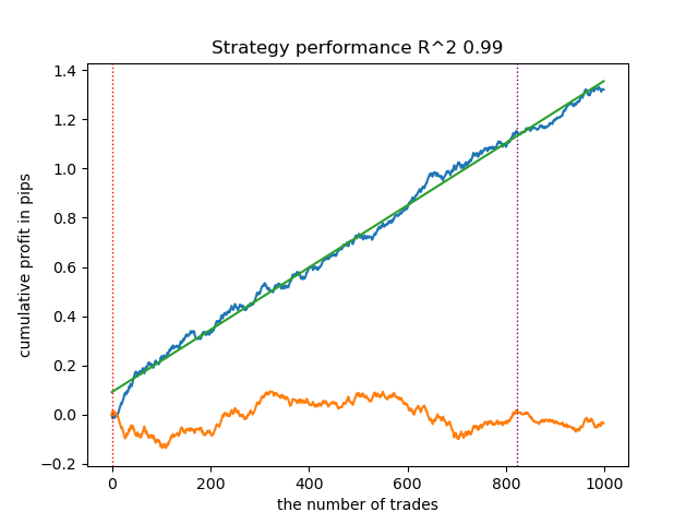
Fig. 5. Testing an algorithm based on fractal markup

There is a direct relationship between the correlation threshold and trading results on new data. For example, for a threshold of 0.7, the balance graph already indicates clear overfitting. This reflects the fact that weak correlation between two parts of a time series leads to weak dependence. Weak dependence, in turn, does not allow for the correct classification of reliable patterns, because they are mixed with unreliable ones.

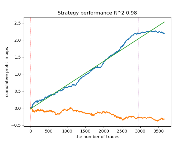
Fig. 6. Testing the algorithm with a threshold of 0.7

It seems that correct pattern identification is critical. Further research and insights are needed on how best to organize the search for fractal structures.

The quality and quantity of features also influence the classification results. If we use increments instead of standard deviations, the balance chart will look different.

It is also necessary to analyze and reasonably criticize the method of labeling trades based on the patterns found.

Error analysis of CatBoost models shows that the models are trained with low error:

>>> models[-1][1].get_best_score()['validation']
{'Accuracy': 0.9700523560209424, 'Logloss': 0.17002244404784328}
>>> models[-1][2].get_best_score()['validation']
{'Logloss': 0.25629795409043277, 'F1': 0.8455473098330242}
>>> 

Exporting and testing models in the MetaTrader 5 terminal

To export models, we need to call the function:

export_model_to_ONNX(model = models[-1],
                     symbol = hyper_params['symbol'],
                     periods = hyper_params['periods'],
                     periods_meta = hyper_params['periods'],
                     model_number = hyper_params['model_number'],
                     export_path = hyper_params['export_path'])

After exporting and compiling the EA, we obtained the following results:

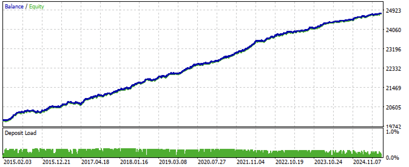
Fig. 7. Testing the EA for the entire period

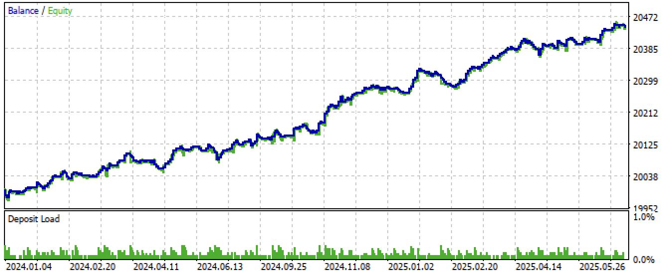
Fig. 8. Testing the EA on new data

Conclusion

In this article, we have touched upon the intriguing topic of fractal analysis and market forecasting using machine learning. These are just the first steps towards exploring the diverse fractal structures that form on financial price charts.

It should be noted that correlation searches may not fully reflect the relationships between past and future price series, and this topic requires further research. For example, regression analysis may be more appropriate than correlation analysis. At the same time, the current algorithm is capable of demonstrating good predictive capabilities when properly configured, which confirms the presence of fractal self-similar structures in financial time series.

The Python files.zip archive contains the following files for development in the Python environment:

Filename	Description
fractal patterns.py	The main script for training models
labeling_lib.py	Updated trade-labeling module
tester_lib.py	Updated custom strategy tester based on machine learning
export_lib.py	Module for exporting models to the terminal
EURUSD_H1.csv	Quote data exported from MetaTrader 5

The MQL5 files.zip archive contains files for the MetaTrader 5 terminal:

Filename	Description
fractal trader.ex5	The compiled bot from the article
fractal trader.mq5	Bot source code from the article
Include//Trend following folder	The ONNX models and the header file for connecting to the bot