Exploring Conformal Forecasting of Financial Time Series

Introduction

MAPIE (Model agnostic prediction interval estimator) is an open-source Python library designed for quantifying uncertainty and managing risk in machine learning models. It allows computing prediction intervals for regression problems, as well as prediction sets for classification and time series. This uncertainty assessment is performed based on a special "calibration set" of data.

One of the key advantages of MAPIE is its model-agnostic nature, which means the library can be used with any model that is compatible with the scikit-learn API, including models developed using TensorFlow or PyTorch, through appropriate wrappers. This property greatly simplifies integration into existing analytical pipelines, as traders often use a variety of machine learning models, from traditional statistical approaches to complex neural networks, depending on the specific asset class or trading strategy. The ability to seamlessly use proven models to incorporate uncertainty quantification significantly reduces implementation costs and accelerates adoption, which is particularly valuable in a dynamic financial environment.

The library is part of the scikit-learn-contrib ecosystem and builds on conformal forecast and distribution-free inference. It implements peer-reviewed algorithms that are model- and use-case-independent and have theoretical guarantees with minimal assumptions about the data and model. Beyond standard classification, MAPIE is also capable of risk control for more complex tasks such as multi-class classification and image segmentation in computer vision by providing probabilistic guarantees on metrics such as recall and precision.

The ability to control risks and provide probabilistic assurance positions MAPIE not simply as a tool for quantifying uncertainty, but as a comprehensive risk management framework. In finance, point forecasts are insufficient because they do not convey the level of confidence or potential error. Providing guaranteed coverage, such as 95% coverage, translates directly into quantifiable risk. This allows risk managers to set explicit risk tolerances.

For example, if the model generates a buy signal, but the conformal forecast indicates a high probability of error, the risk manager may decide to reduce the position or abstain from the trade, directly controlling the potential loss. This supports more robust decision-making under uncertainty going beyond simple forecast accuracy.

Basic principles of conformal forecasting: model-agnostic guarantees independent of distribution

Conformal prediction (CP) is a statistical framework that generates prediction sets for classification problems or prediction intervals for regression with guaranteed coverage probabilities. This means that at a given confidence level, say 90%, the true result will be in the predicted set or interval at least 90% of the time.

The key advantage of CP is its "distribution-free" nature: the method does not rely on strict assumptions about the underlying distribution of the data or the model itself. The only fundamental assumption is that the data (training and test points) are exchangeable, that is, they are taken from the same distribution, and their order does not matter.

This assumption is weaker than the independence and identical distribution (i.i.d.) assumption and can often be justified in practice. Unlike traditional prediction intervals, which can only approximate coverage, the CP offers guarantees for finite samples, ensuring that the specified level of coverage is achieved even with limited data.

The distribution-independent guarantee of conformal forecasting directly addresses the fundamental problem of financial modeling. Financial data are notoriously non-normally distributed, exhibit heavy tails, and often violate typical statistical assumptions, such as homoscedasticity or independence of increments.

Traditional prediction intervals often rely on these assumptions, such as normal residuals, and thus provide only approximate coverage. The ability of the CP to provide the guaranteed coverage without such assumptions make it inherently more robust and trustworthy for financial applications where misspecified distributions can lead to significant underestimation of risk. This means that the reported confidence levels are more reliable in real-world, complex financial datasets.

Conformal forecasting typically involves using a trained machine learning model, creating a calibration dataset (unseen by the model during training), computing "conformity scores" on this set, and then using the quantile of these scores to determine the prediction sets. Moving from the approximate coverage to the guaranteed finite-sample coverage fundamentally changes the regulatory and risk management landscape for machine learning models in finance.

In high-risk industries, such as finance, models often need to demonstrate quantitative robustness and control over error rates. This differs from traditional statistical methods, where "90% confidence" may only be an asymptotic property or approximation. For a quantitative trader, this provides a more solid basis for justifying trading strategies or risk capital allocation.

Prediction sets versus point predictions in binary classification

Traditional binary classification models output a single predicted label (e.g., "Buy" or "Sell") or a probability score (e.g., 0.8 for "Buy"). These are point forecasts. However, conformal forecasting provides prediction set, which is a subset of the possible classes (for example, {Buy}, {Sell} or {Buy, Sell}). This set is guaranteed to contain the true label with a given probability.

For binary classification, the prediction set can be:

• A single class (e.g. {Buy} or {Sell}), indicating a high degree of confidence.
• Both classes (e.g. {Buy, Sell}), indicating uncertainty or ambiguity.
• An empty set {} (though this is less common when using some methods such as APS, and is often undesirable), which indicates extreme uncertainty or that no class meets the confidence threshold.

The "informativeness" of a prediction set is inversely proportional to its size: smaller sets (e.g., one-class) are more informative than larger sets (e.g., both classes). Explicit output of a set instead of a single point fundamentally changes decision-making in binary classification for finance. Instead of a simple yes/no or buy/sell signal, the forecast set provides a direct measure of the model's confidence.

A one-class set such as {Buy} suggests a strong signal, while a two-class set {Buy, Sell} indicates significant ambiguity. This allows for a more nuanced trading strategy: taking trades on high confidence signals and either holding off, reducing position size, or seeking further information for ambiguous signals. It is a direct mechanism for integrating uncertainty into effective financial decisions.

The "information content" of forecast sets becomes a direct measure of efficiency and risk tolerance in financial trading. A broad, uninformative prediction set (e.g., {Buy, Sell}) for a transaction means that the model cannot reliably distinguish between a buy and a sell at the desired level of confidence. For a quantitative analyst, this is not a forecasting error that needs to be corrected, but a signal to avoid any action or act with extreme caution. This allows for dynamic risk management: allocating more capital to trades with narrow, highly reliable sets and preserving capital by avoiding or minimizing exposure to trades with broad, uncertain sets. This directly leads to the optimization of the risk-reward profile of the trading strategy.

Theoretical guarantees: marginal and conditional coverage

Conformal predictors are "automatically valid" in the sense that their prediction sets have a coverage probability equal to or greater than a given confidence level (1 - α) on average for all data This guarantee holds regardless of the underlying model or data generation, provided the exchangeability assumption is met. This property is known as marginal coverage.

While marginal coverage is guaranteed, it is an average figure. More rigorous concepts, such as conditional validity, strive for coverage guarantees based on specific data properties (e.g. by class, by object, by label). Inductive conformal predictors (computationally efficient version) primarily control unconditional probability of coverage. Achieving conditional validity often requires method modifications.

The difference between marginal and conditional coverage is of paramount importance for financial binary classification, especially with unbalanced data sets common in finance (e.g., many "no deal" or "hold" signals compared to fewer "buy" or "sell" signals).

Marginal coverage ensures that, on average, 90% of forecasts will be correct. However, if buy signals are rare, the model can achieve 90% marginal coverage, being very accurate on sell signals but performing poorly on buy signals. This can lead to significant missed opportunities or losses if buy signals are critical.

Conditional coverage, especially class coverage, ensures that the desired level of confidence is achieved for each class individually. This is crucial to ensure the reliability of forecasts for both buy and sell trades, preventing systematic biases that can undermine a trading strategy.

Striving for conditional validity using methods, such as Mondrian Conformal Prediction, directly addresses the fairness and reliability issue for various classes of results in financial applications. In finance, forecasting errors in certain classes (e.g., a rare but highly profitable "buy" opportunity or a critical "sell" to avoid large losses) can have disproportionately high costs compared to forecasting errors in more common "no deal" scenarios.

By providing conditional coverage, the system guarantees a minimum level of reliability for each type of transaction rather than the average one. This allows for fairer treatment of different trading signals and increases confidence in the model's ability to handle a variety of market conditions and rare events, which is essential for robust algorithmic trading.

Conformity scores: the core of conformal prediction

Conformity scores are the core of conformal prediction; they quantify how "unusual" or "out of line" a new data point is compared to the calibration data. The only requirement for the scoring function is that higher scores should encode a worse match between the input data and its hypothetical label. These estimates are used to calculate a quantile (cutoff point) from the calibration set, which then defines a prediction set for new test points.

MAPIE implements a variety of conformity scores, including symmetric (e.g., Absolute Residual Score for regression) and asymmetric (e.g., Gamma Score for regression), which affect how prediction interval bounds are calculated. Specific assessments, such as LAC, APS and RAPS, are used for classification.

The choice of conformity assessment is not just a technical detail, but rather a strategic decision, which affects the practical usefulness and interpretability of prediction sets. Different conformity scores (e.g., LAC, APS) lead to different behavior when generating prediction sets.

For example, LAC may produce empty sets under high uncertainty, which may be undesirable in finance since it provides no guidance. APS by design avoids empty sets by always providing some set of plausible outcomes. This means that the choice of score directly influences how "bad" samples are represented and whether the system can always provide an effective (albeit vague) answer. A quantitative trader should choose a valuation that matches the desired level of information content and risk tolerance.

The concept of "conformity" allows us to identify an "outlier" or "unusual" observation in the context of a data-driven model's predictions, which is highly relevant for detecting abnormal trading conditions. In financial markets, unusual price movements, sudden surges in volume, or unexpected news can result in data points that deviate significantly from historical patterns.

A high conformity score for a new observation would signal that the observation "does not fit" the patterns observed in the calibration data. This can serve as an early warning system for market anomalies or regime shifts, prompting a revision of the trading strategy or a temporary suspension of automated trading, thereby acting as a critical risk management tool that goes beyond simple model accuracy.

A detailed consideration of the relevant conformity scores for classification

MAPIE offers various conformity scores, each with its own characteristics and applicability.

• Least Ambiguous Set-valued Classifier (LAC):

1. Calculation: The conformity score is defined as 1 - softmax_score_of_the_true_label.
2. Properties: a simple approach that theoretically guarantees marginal coverage. Typically results in small prediction sets.
3. Applicability/limitations: Tends to form empty prediction sets when there is high model uncertainty (e.g. near decision boundaries). This can be problematic in finance, as an empty set does not provide actionable guidance.

• Adaptive Prediction Sets (APS):

1. Calculation: Conformity scores are calculated by summing the ranked softmax scores of each label, from highest to lowest, until the true label is reached.
2. Properties: Overcomes the problem of empty LAC sets; prediction sets are not empty by definition. Provides marginal coverage guarantees.
3. Applicability: More robust for financial applications, where some form of prediction (even if uncertain) is always preferable to an empty set.

• Regularized Adaptive Prediction Sets (RAPS):

1. Calculation: Similar to APS, but includes a regularization term to reduce the size of prediction sets.
2. Properties: Aims to balance coverage and efficiency by regularizing the set size while maintaining coverage guarantees.
3. Applicability: Useful in scenarios where forecast set size (effectiveness) is as important as coverage, as smaller sets are more effective in trading.

• Mondrian Conformal Prediction:

1. Calculation: This method calculates individual quantiles of conformity scores for each class. This allows class-aware predictions to be included in the set.
2. Properties: Provides conditional coverage (1 - α) for each class, which is vital for unbalanced multi-class or binary problems.
3. Applicability: Highly recommended for financial binary classification (buy/sell) where the classes may be unbalanced (e.g. fewer "buy" signals than "hold" or "sell") or have different error tolerances. This ensures that the reliability of the buy signal is guaranteed regardless of the sell signal.

The evolution of conformity scores from LAC to APS/RAPS reflects the practical need for effective and informative prediction sets in real-world applications. While LAC is conceptually simple, its tendency to create empty sets is a significant financial drawback. An empty forecast set for a buy/sell decision provides no guidance, effectively stopping the decision-making process. APS and RAPS, by guaranteeing non-empty sets, ensure that even under high uncertainty the model provides some plausible results, allowing for a default decision to "hold" or "reassess" rather than stopping completely. This ensures continuous operations and risk management.

The Mondrian method is a critical advancement for financial binary classification, directly addressing the problem of unbalanced classes and differential influence of errors. In buy/sell scenarios, "buy" signals may be rare but very profitable, while "sell" signals may be more frequent but less significant individually. Standard conformal methods provide marginal coverage, which may mean that coverage for the rare "buy" class is lower than desired if the overall average is achieved. Mondrian's ability to calculate class-specific quantiles ensures that the desired confidence level is maintained for each class.

This is crucial to prevent systematic undercoverage of critical, rare events (such as strong buy signals) and thus leads to more reliable and potentially more profitable trading strategies. This ensures that the robustness of the model is not simply an average, but is maintained for the specific type of transaction under consideration.

Stages of forming conformal predictive sets for classification

Let's break down the process step by step:

1. Selecting a measure of nonconformity (or "scoring function"): This is extremely important. Classification often uses the output of a pre-trained classifier (e.g. logistic regression, support vector machines, neural network, or random forest). Let f(x) be the output of the classifier for the x input. If f(x) outputs probabilities (e.g. from a softmax layer), a good measure of non-conformity for a data point (xi ,yi) might be:
• 1 - predicted probability of the true class: αi =1−P^(yi ∣xi ). Here P^(yi ∣xi ) is the predicted probability of the true label yi for the xi input data. A small value of αi means that the model is confident in its prediction for the true class, indicating "conformity". A large αi means that the model is less confident, indicating "non-conformity".
• Based on softmax temperature scaling: If the model produces logits, softmax can be applied to obtain probabilities. Then the non-conformity estimate will again be 1−P(yi ∣xi).
• Distance to the decision boundary (for SVM): For models like SVM that output a signed distance to the decision boundary, the non-conformity measure can be associated with a negative value of this distance for correctly classified points or a positive value of this distance for incorrectly classified points.
2. Data splitting for calibration: To make predictions statistically reliable, we need to calibrate our estimates of nonconformity. This is usually done by splitting the original dataset into two parts:
• Training set: Used to train the base classifier (e.g. neural network, SVM).
• Calibration sample: A separate set of data points not used for training the classifier, but used to calculate non-conformity scores and determine the reliability threshold.
3. Calculating nonconformity estimates for calibration data: For each (xj ,yj) data point in the calibration sample, its αj nonconformity score is calculated using a pre-trained classifier.
4. Sorting non-conformity scores and determining the quantile (1−δ): All non-conformity estimates from the calibration sample are sorted in ascending order: α(1) ≤α(2) ≤⋯≤α(m), where m is the size of the calibration sample.
   Now the desired significance level δ∈(0,1) is selected. This δ represents the probability that the predictive set contains no true mark. Conversely, 1−δ is the desired coverage probability. We need to find the (1−δ)th quantile of these estimates. More precisely, the smallest value of q is found such that at least (1−δ)×(m+1) calibration scores are less than or equal to q. A common way to calculate this threshold: q=α(⌈(m+1)(1−δ)⌉)
   However, for finite samples, it is often more reliable to consider the empirical quantile (1−δ) adjusted for finite samples to ensure accurate coverage. A more practical approach is to find the smallest α(k) such that k/(m+1)≥1−δ. Let this value be q^.
5. Forming a predictive set for a new test point: Let xtest be the new input we want to make a prediction for. For each possible label of k in a set of classes (for example, 1,2,…,C for C classes), imagine that ytest =k.
   Now the nonconformity score of αtest,k is calculated for the (xtest ,k) pair using the chosen non-conformity measure (for example, 1−P^(k∣xtest )).
   The predictive set of Ytest for xtest is formed by including all k labels, for which the nonconformity score of αtest,k is less than or equal to the q^ threshold determined in step 4: Ytest ={k∈{1,…,C}∣αtest,k ≤q^ }

MapieClassifier key components

MapieClassifier is the core class in MAPIE for generating prediction sets in classification problems. It is designed to be compatible with any scikit-learn estimator that has fit, predict, and predict_proba methods. If no estimator is provided, LogisticRegression is used by default.

The cv parameter allows using different cross-validation strategies (e.g., "split", "crossval", "prefit") to calculate conformity scores, influencing the difference between the jackknife and CV methods. The "prefit" option assumes that the estimator has already been trained, and all provided data is used to calibrate the predictions by computing scores. The process involves splitting the data into training, calibration, and test sets, training a baseline model on the training set, and then using MAPIE to "conformalize" the model on the calibration set.

The cv="prefit" option is very practical for financial applications where models are often continuously trained or refitted on large datasets. In real-time or high-frequency trading, models are frequently updated or trained on streaming data. The ability to use a pre-trained model and then calibrate it with a separate dataset means that the computationally intensive training step does not need to be repeated for conformal prediction. This allows uncertainty quantification to be efficiently integrated into existing high-performance trading systems without significant delays.

The 'method' parameter (now deprecated in favor of conformity_score) specifies the conformal prediction method. The removal of the 'method' parameter in favor of conformity_score represents a move towards greater modularity and explicit control over the underlying conformal prediction mechanism. This architectural solution allows users to precisely determine, how the "mismatch" for their particular problem is measured. For financial data, where different types of errors or uncertainties may be more critical (e.g., misclassifying a "buy" versus a "sell"), this modularity allows the uncertainty quantification process to be fine-tuned to better suit specific financial risk metrics or trading objectives. This gives advanced users the ability to customize conformal prediction beyond the predefined methods.

Conclusions on the theoretical part and recommendations

The MAPIE library is a powerful tool for quantifying uncertainty in machine learning models, especially in the context of conformal binary classification for financial applications. Its ability to provide distribution-independent, finite-sample coverage guarantees and explicitly identify "good" and "bad" samples significantly improves the reliability and manageability of risks in high-risk financial environments.

MAPIE's ability to integrate with any scikit-learn-compatible model provides flexibility and reduces barriers to adoption in existing financial systems. Moving from point forecasts to forecast sets allows for more nuanced and informed decisions by explicitly accounting for the degree of model uncertainty. In particular, the distinction between marginal and conditional coverage is crucial for financial applications, where the reliability of forecasts for rare but critical classes (e.g., strong buy signals) may be of disproportionate importance.

Recommendations:

• Conformity assessment priority: For binary classification in finance, it is recommended to prefer conformity estimators, such as APS or RAPS, as they guarantee non-empty prediction sets, which ensures the continuity of the decision-making process and always provides some form of actionable inference, even under high uncertainty.
• Using Mondrian Conformal Prediction: In scenarios with imbalanced classes or when conditional coverage for specific types of transactions (e.g. rare buy signals) is critical, the Mondrian Conformal Prediction method should be considered. This method provides reliability guarantees for each class individually, preventing systematic undercoverage of important but rare events.
• Rigorous time series validation: The application of conformal forecasting to financial time series requires careful validation and consideration of the violation of the exchangeability assumption. While MAPIE has specialized time series tools, such as the MapieTimeSeriesRegressor, they should be combined with other time series-specific methods and rigorous backtesting to ensure robustness in the face of non-stationarity and sudden market changes.
• Development of multi-level trading strategies: Trading strategies should be developed that exploit the interpretability of forecast sets. This will allow dynamic adjustment of risk exposure: for example, to execute high-confidence trades (single-class sets) with full capital, and for low-confidence trades (multi-class sets) to reduce the position size, apply hedging, or abstain.

Practical application of the MAPIE library

The MAPIE library implements two methods for "conforming" model predictions:

• Split conformal predictions
• Cross conformal predictions

The first method divides the original data into training and validation subsamples. The first one is used to train the base classifier, and the second one is used to calibrate and output prediction sets. The second method splits the dataset into multiple folds and uses cross-training and calibration. We will use the second one straight away, since it should be more reliable due to cross-validation. This is similar in spirit to walk-forward validation for readers unfamiliar with cross-validation.

First, we need to install the MAPIE package and import the module:

pip install mapie
from mapie.classification import CrossConformalClassifier

Additional libraries, listed below, should also be installed and imported.

import pandas as pd
import math
from datetime import datetime
from catboost import CatBoostClassifier
from sklearn.model_selection import train_test_split
from sklearn.model_selection import cross_val_predict
from sklearn.model_selection import StratifiedKFold
from bots.botlibs.labeling_lib import *
from bots.botlibs.tester_lib import test_model
from mapie.classification import CrossConformalClassifier
from sklearn.ensemble import RandomForestClassifier

Next, I wrote a test function that implements conformal prediction and then outputs bad and good examples based on the prediction sets.

def meta_learners_mapie(n_estimators_rf: int,
                       max_depth_rf: int,
                       confidence_level: float = 0.9):
    
    dataset = get_labels(get_features(get_prices()), markup=hyper_params['markup'])
    data = dataset[(dataset.index < hyper_params['forward']) & 
                  (dataset.index > hyper_params['backward'])].copy()
    
    # Extract features and target
    feature_columns = list(data.columns[1:-2])
    X = data[feature_columns]
    y = data['labels']

    mapie_classifier = CrossConformalClassifier(
                        estimator=RandomForestClassifier(n_estimators=n_estimators_rf, 
                                                         max_depth=max_depth_rf),
                        confidence_level=confidence_level,
                        cv=5,
                        ).fit_conformalize(X, y)
    predicted, y_prediction_sets = mapie_classifier.predict_set(X)
    
    
    y_prediction_sets = np.squeeze(y_prediction_sets, axis=-1)
    # Calculate set sizes (sum across classes for each sample)
    set_sizes = np.sum(y_prediction_sets, axis=1)
    # Initialize meta_labels
    data['meta_labels'] = 0.0
    # Mark labels as "good" (1.0) only where prediction set size is exactly 1
    data.loc[set_sizes == 1, 'meta_labels'] = 1.0
    # Report statistics on prediction sets
    empty_sets = np.sum(set_sizes == 0)
    single_element_sets = np.sum(set_sizes == 1)
    multi_element_sets = np.sum(set_sizes >= 2)
    
    print(f"Empty sets (meta_labels=0): {empty_sets}")
    print(f"Single element sets (meta_labels=1): {single_element_sets}")
    print(f"Multi-element sets (meta_labels=0): {multi_element_sets}")

    # Return the dataset with features, original labels, and meta labels
    return data[feature_columns + ['labels', 'meta_labels']]

We will use the random forest from scikit-learn as the base classifier, since the MAPIE package supports all classifiers from this package. Random forest is a fairly powerful model with flexible settings, but you can use another model that you consider appropriate for your tasks. To do that, we should pass any other classifier as estimator in the highlighted code. It is worth noting that this classifier will only be used to output predictive sets, while CatBoost will still be trained as the final models. 

Let's break down the meta_learners_mapie() function step by step.

Definition of a function and its parameters:

def meta_learners_mapie(n_estimators_rf: int,
                       max_depth_rf: int,
                       confidence_level: float = 0.9):

The function takes three arguments:  

1. n_estimators_rf - number of trees in the Random Forest to be used as the base model.  
2. max_depth_rf - maximum depth of each tree in the random forest.  
3. confidence_level - confidence level for conformal prediction (default 0.9, i.e. 90%). This parameter determines how "wide" the predictive sets will be.

Loading and preparing data:

dataset = get_labels(get_features(get_prices()), markup=hyper_params['markup'])
data = dataset[(dataset.index < hyper_params['forward']) &
              (dataset.index > hyper_params['backward'])].copy()

First, the data is loaded and pre-processed.

It is assumed that there are three auxiliary functions:  

• get_prices() - load the raw data (prices) 
• get_features() - extract or compute features from the data returned from get_prices() 
• get_labels() - generate target labels based on the features and the 'markup' parameter from the hyper_params dictionary.  

The data is then sorted by the time index. Only those records whose index is between hyper_params['backward'] and hyper_params['forward'] are kept.  .copy() is used to create a copy of the filtered DataFrame to avoid problems with SettingWithCopyWarning.

Extracting X features and y target variable:

feature_columns = list(data.columns[1:-2])
X = data[feature_columns]
y = data['labels']

• feature_columns - create a list of column names to be used as features. All columns are taken except the first (index 0) and the last two. This is specific to the 'data' structure. 
• X - create DataFrame with features by selecting columns from feature_columns.  
• y - create Series with target labels from the 'labels' column.

Initialization and training of the MAPIE conformal classifier:

mapie_classifier = CrossConformalClassifier(
                    estimator=RandomForestClassifier(n_estimators=n_estimators_rf,
                                                     max_depth=max_depth_rf),
                    confidence_level=confidence_level,
                    cv=5,
                    ).fit_conformalize(X, y)

• An instance of CrossConformalClassifier from the MAPIE library is created. This is a wrapper that adds conformal prediction capabilities to any scikit-learn-compatible model.  
• estimator - RandomForestClassifier from scikit-learn is used as the base model (estimator). It receives n_estimators_rf and max_depth_rf parameters obtained by the function.  
• confidence_level - use the confidence level passed to the function.  cv=5 - indicate the use of 5-fold cross-validation to calibrate the conformal predictor. This is the standard approach in MAPIE to split data into training and calibration sets.  
• .fit_conformalize(X, y) - the method trains a base RandomForestClassifier on (X, y) data and simultaneously calibrates the conformal predictor. After this step, mapie_classifier is ready to make conformal predictions.

Obtaining predictions and prediction sets:

predicted, y_prediction_sets = mapie_classifier.predict_set(X)

mapie_classifier.predict_set(X) - generates two outputs for the X inputs:  

• predicted - point predictions (one class per example), similar to the standard .predict() method.  
• y_prediction_sets - key output of conformal prediction. For each data sample, this is an array (or list of arrays) indicating which classes are included in the predictive set with the given confidence_level. A predictive set is a set of classes that contains the true class with the probability of at least confidence_level. Its usual form is (n_samples, n_classes, 1) or (n_samples, n_classes), where the values are Boolean (True/False) or 0/1 indicating the inclusion of the class in the set.

Handling predicted sets:

y_prediction_sets = np.squeeze(y_prediction_sets, axis=-1)
set_sizes = np.sum(y_prediction_sets, axis=1)

• np.squeeze(y_prediction_sets, axis=-1): if y_prediction_sets has an extra dimension of size 1 at the end (for example, (n_samples, n_classes, 1)), this operation removes it, resulting in (n_samples, n_classes).  
• set_sizes = np.sum(y_prediction_sets, axis=1): for each sample (along axis 0), the values in y_prediction_sets are summed across classes (along axis 1). If y_prediction_sets contains 0/1, then this sum provides the number of classes included in the prediction set for each example. That is, set_sizes is an array of predictor set sizes for each observation.

Generating meta tags:

data['meta_labels'] = 0.0
data.loc[set_sizes == 1, 'meta_labels'] = 1.0

• data['meta_labels'] = 0.0: a new column 'meta_labels' is added to the DataFrame data and initialized to zero.  
• data.loc[set_sizes == 1, 'meta_labels'] = 1.0: a key step to create meta labels. For those examples where the prediction set size (set_sizes) is exactly 1 (i.e. the model predicts exactly one class with the given confidence), the value in the 'meta_labels' column is set to 1.0. This means that for these examples, the model is very confident in its single predicted class. If the predictive set is empty (size 0) or contains multiple classes (size >= 2), the meta label remains 0.0.

Report on predicted sets statistics:

empty_sets = np.sum(set_sizes == 0)
single_element_sets = np.sum(set_sizes == 1)
multi_element_sets = np.sum(set_sizes >= 2)

print(f"Empty sets (meta_labels=0): {empty_sets}")
print(f"Single element sets (meta_labels=1): {single_element_sets}")
print(f"Multi-element sets (meta_labels=0): {multi_element_sets}")

The following quantities are calculated:  

• empty_sets - empty prediction sets (the model cannot choose any class with the given confidence).  
• single_element_sets - sets containing exactly one class (high-confidence predictions with meta_labels=1).  
• multi_element_sets - sets containing two or more classes (the model is unsure about one particular class).  

These statistics are printed out, giving an idea of how often the model generates confident, unambiguous predictions.

Returning the result:

return data[feature_columns + ['labels', 'meta_labels']]

The function returns a DataFrame containing the original features (feature_columns), the original labels ('labels'), and the newly generated meta labels ('meta_labels'). These meta labels can then be used, for example, to train another model (meta model) or to select only the most reliable predictions for further action.

Ultimately, the function uses conformal prediction to identify those observations for which the baseline model (Random Forest) makes a prediction with high confidence, specifying exactly one possible class. These observations are labeled with a "meta label" equal to 1.

Improving the conformation prediction function

After testing the function and evaluating the results, I came to the conclusion that it has one significant drawback. While it does a great job of inferring the predictive sets on which the final meta model is trained, the base model is still trained on the original dataset, which may contain many errors, making it poorly generalizable to new data. The meta model corrects the errors of the base model by prohibiting it from trading in situations with high uncertainty, but due to the weak generalization of the base model, the entire system still performs poorly in a non-stationary market.

Let's recall that after training the MAPIE classifier, we get two sets of labels: model predictions (the labels themselves) and predictive sets.

predicted, y_prediction_sets = mapie_classifier.predict_set(X)

The initial conformal prediction function uses only the predictive sets to train the meta model, while the base model is trained on the labels from the original dataset. But we can also fix the labels for the base model, leaving only those that the MAPIE classifier has the most confidence in.

# Initialize meta_labels column with zeros
data['meta_labels'] = 0.0
# Set meta_labels to 1 where predicted labels match original labels
# Compare predicted values with the original labels in the dataset
data.loc[predicted == data['labels'], 'meta_labels'] = 1.0

In the code above, we compare the predicted labels with the original ones and form a new 'meta_labels' column, which contains ones if the labels match and zeros if they do not match. We will then train the base classifier only on those examples whose labels match.

The first part of the final model training function will now look like this:

def fit_final_models(dataset) -> list:
    # features for model\meta models. We learn main model only on filtered labels 
    X = dataset[dataset['meta_labels']==1]
    X = X[X.columns[1:-3]]
    X_meta = dataset[dataset.columns[1:-3]]
    # labels for model\meta models
    y = dataset[dataset['meta_labels']==1]
    y = y[y.columns[-3]]
    y_meta = dataset['conformal_labels']

Thus, both models will return higher-quality outputs after training as far as possible on non-stationary time series.

Training and testing the algorithm

To test the method, we will train 10 models in a cycle on the EURUSD currency pair from the beginning of 2020 to the beginning of 2025. The remaining data is the forward period.

hyper_params = {
    'symbol': 'EURUSD_H1',
    'export_path': '/Users/dmitrievsky/Library/Program Files/MetaTrader 5/MQL5/Include/Trend following/',
    'model_number': 0,
    'markup': 0.00010,
    'stop_loss':  0.00500,
    'take_profit': 0.00200,
    'periods': [i for i in range(5, 300, 30)],
    'backward': datetime(2020, 1, 1),
    'forward': datetime(2025, 1, 1),
}

models = []
for i in range(10):
    print('Learn ' + str(i) + ' model')
    models.append(fit_final_models(meta_learners_mapie(15, 5, confidence_level=0.90, CV_folds=5)))

The meta_leaners_mapie function will be called with the following arguments:

• 15 decision trees in Random Forest (base classifier)
• 5 - the depth of each decision tree
• model confidence level is 90%
• the number of folds for cross-validation is five

During training the following information is displayed:

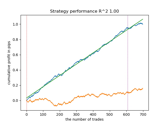
Learn 9 model
Empty sets (meta_labels=0): 0
Single element sets (meta_labels=1): 6715
Multi-element sets (meta_labels=0): 22948
Correct predictions (meta_labels=1): 16638
Incorrect predictions (meta_labels=0): 13025
R2: 0.9931613891107195

• Empty sets - the number of empty predictive sets when the model is not confident in any of the classes
• Single element sets - number of predictive sets that contain a single element. The model is confident in these predictions with a probability of 0.9
• Multi-element sets - number of predictive sets that contain multiple classes. The model is not confident in these examples
• Correct predictions - the number of correctly predicted labels
• Incorrect predictions - the number of incorrectly predicted labels
• R2 - quality metric for the balance curve

Based on the provided report, it can be concluded that the dataset contains a lot of junk data: 6,715 reliable predictions versus 22,948 unreliable ones. But our model will try to fix this and will only use reliable ones. As a result, the balance graph in the tester will look like this.

A distinctive feature of this algorithm is that both models (main and meta) are trained with high Accuracy:

>>> models[-1][1].get_best_score()['validation']
{'Accuracy': 0.92, 'Logloss': 0.1990666082064606}

>>> models[-1][2].get_best_score()['validation']
{'Accuracy': 0.9647435897435898, 'Logloss': 0.10955056411224594}

This means that a large portion of the uncertainty has now been removed from the models compared to the original dataset, which contains a lot of junk data. Additionally, the final models can be calibrated to obtain more reliable decision thresholds, which is beyond the scope of this article.

What happens if the confidence_level is reduced from 0.9 to 0.6? We will get more sets that contain the true class label with 60% probability, this is reflected in the report.

Learn 8 model
Empty sets (meta_labels=0): 0
Single element sets (meta_labels=1): 28647
Multi-element sets (meta_labels=0): 991
Correct predictions (meta_labels=1): 16999
Incorrect predictions (meta_labels=0): 12639
R2: 0.9850582205528567

While in the previous example 'Single Element sets' contained few examples, now their number prevails over 'Multi-element sets'. But the confidence in a successful outcome is much lower. The balance chart reflects this uncertainty because it contains more drawdowns.

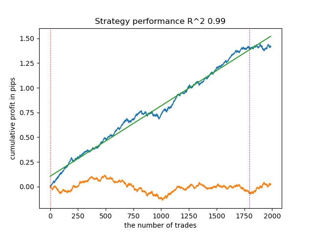
Thus, by adjusting the confidence level of the model, it is possible to control the risks associated with unsuccessful trading operations. This makes it possible to seek a compromise between the number of transactions and the efficiency of trading, or the probability of a black swan event.

Exporting and testing models in the Meta Trader 5 terminal

Exporting models is implemented in exactly the same way as in all previous articles. Read them for more detailed information.

export_model_to_ONNX(model = models[-1],
                     symbol = hyper_params['symbol'],
                     periods = hyper_params['periods'],
                     periods_meta = hyper_params['periods'],
                     model_number = hyper_params['model_number'],
                     export_path = hyper_params['export_path'])

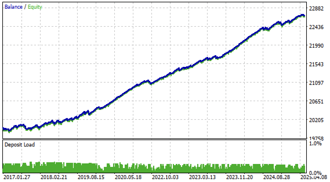
Now we can test the algorithm in the Meta Trader 5 terminal. The trading system proved to be stable not only in the forward period, but also in the past period, from 2017 to 2020.

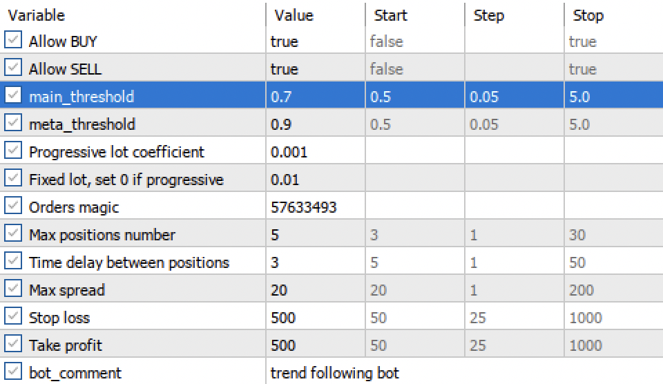
'main threshold' and 'meta threshold' settings now allow us to filter model signals by confidence. The higher the threshold, the more confident the trading, but the fewer transactions.

Conclusion

In this article, we introduced conformal predictions and the MAPIE library that implements them. This approach is one of the most modern ones in machine learning and allows us to focus on risk management for existing diverse machine learning models. Conformal predictions, by themselves, are not a way to find patterns in data. They only determine the degree of confidence of existing models in predicting specific examples and allow filtering for reliable predictions. This important property allows managing risk in trading by adjusting the confidence threshold at the model training stage.

The Python files.zip archive contains the following files for development in the Python environment:

Filename	Description
mapie causal.py	The main script for training models
labeling_lib.py	Updated module with trade labeling module
tester_lib.py	Updated custom strategy tester based on machine learning
export_lib.py	Module for exporting models to the terminal
EURUSD_H1.csv	The file with quotes exported from the MetaTrader 5 terminal

The MQL5 files.zip archive contains files for the MetaTrader 5 terminal:

Filename	Description
mapie trader.ex5	The compiled bot from the article
mapie trader.mq5	Bot source code from the article
Include//Trend following folder	The ONNX models and the header file for connecting to the bot