Hidden Markov Models in Machine Learning-Based Trading Systems

MetaTrader 5 — Trading | 20 April 2026, 13:27

252

[Deleted]

Introduction

Hidden Markov models (HMMs) are a powerful class of probabilistic models designed to analyze sequential data, where observed events depend on some sequence of unobserved (hidden) states that form a Markov process.HMMs are doubly stochastic models characterized by a finite set of hidden states and a sequence of observable events whose probability depends on the current hidden state.The main assumptions of HMM include the Markov property for hidden states, meaning that the probability of transition to the next state depends only on the current state, and the independence of observations given knowledge of the current hidden state.

Hidden Markov models have found wide application in various fields, including speech and image recognition, natural language processing (e.g., part-of-speech tagging), bioinformatics (DNA and protein sequence analysis), and time series analysis (forecasting, anomaly detection). The ability to model systems whose internal structure is not directly observable but influences observable outputs makes HMM a valuable tool for analyzing complex time-dependent relationships. Observations in such models are only indirect reflections of hidden processes, and understanding these processes can provide important information about the system dynamics.

The hmmlearn library is a set of Python algorithms for unsupervised learning (hidden Markov models). It is designed to provide simple and efficient tools for working with HMMs, following the scikit-learn library API, facilitating integration into existing machine learning projects and simplifying the training process for users familiar with scikit-learn. Hmmlearn is built on top of fundamental scientific Python libraries, such as NumPy, SciPy, and Matplotlib.

hmmlearn key capabilities include the implementation of various HMM models with different emission distribution types, training of model parameters from observed data, inferring the most probable hidden state sequences, generating samples from trained models, and the ability to save and load trained models. The variety of implemented models allows users to select the most appropriate emission distribution type depending on the nature of their data. The data type (continuous, discrete, counters) determines which probability distribution best describes the process of generating observations in each hidden state.

Algorithms in the hmmlearn library

The hmmlearn library implements the following main HMM models:

hmm.CategoricalHMM - for modeling sequences of categorical (discrete) observations.
hmm.GaussianHMM - for modeling sequences of continuous observations assuming a Gaussian distribution in each hidden state.
hmm.GMMHMM - for modeling sequences of continuous observations where the emissions from each hidden state are described by a mixture of Gaussian distributions.
hmm.MultinomialHMM - for modeling sequences of discrete observations, where each state has a probability distribution over a fixed set of symbols.
hmm.PoissonHMM - for modeling data sequences that represent event counters, where emissions from each hidden state follow a Poisson distribution.
vhmm.VariationalCategoricalHMM - variational version of CategoricalHMM that uses variational inference methods for learning.
vhmm.VariationalGaussianHMM - variational version of GaussianHMM designed for continuous observations distributed according to a multivariate normal law and trained using variational inference.

We are interested in the algorithms that work with continuous data, so only they will be considered.

hmm.GaussianHMM class

The hmm.GaussianHMM class in the hmmlearn library implements a hidden Markov model with Gaussian emissions. This model is used when the observed variables are continuous and are assumed to follow a multivariate normal (Gaussian) distribution in each hidden state.

Gaussian HMM is widely used to model various time series, such as financial data (e.g., stock prices), readings from various sensors, and other continuous processes where the observed values can be described by a Gaussian distribution in each of the hidden states.

The hmm.GaussianHMM class constructor takes the following parameters:

n_components (int, default is 1): defines the number of hidden states in the model. Each state will be associated with its own Gaussian distribution.
covariance_type ({"spherical", "diag", "full", "tied"}, default is "diag"): sets the type of covariance matrix used for each state. The choice of covariance type directly affects the complexity of the model and the number of estimated parameters.

spherical - each state uses the same variance for all features. The covariance matrix is a multiple of the identity matrix.
diag - each state uses a diagonal covariance matrix, assuming that features within a state are statistically independent but may have different variances.
full - each state uses a full (unconstrained) covariance matrix, allowing us to model correlations between features within each state. This option is the most flexible, but requires more data for evaluation and may be prone to overfitting.
tied - all hidden states share the same full covariance matrix. This allows for correlations between features to be taken into account, but assumes that the structure of these correlations is the same across all states.

min_covar (float, default is 1e-3): sets the minimum value for the diagonal elements of the covariance matrix to prevent it from becoming degenerate (e.g. zero variance) during training and to avoid overfitting.
startprob_prior (array, form (n_components,), optional): Dirichlet prior parameters for the startprob_ initial probabilities, which determine the probability of starting the observation sequence in each of the hidden states.
transmat_prior (array, form (n_components, n_components), optional): parameters of the Dirichlet prior for each row of the transmat_ transition matrix, which determines the transition probability between hidden states.
means_prior (array, form (n_components,), optional): the mean of the normal prior distribution for the means (means_) of each hidden state.
means_weight (array, form (n_components,), optional): weight (or precision, inverse variance) of the normal prior distribution for the means (means_) of each hidden state.
covars_prior (array, form (n_components,), optional): parameters of the prior distribution for the covars_ covariance matrix. The type of this distribution depends on the covariance_type parameter. For "spherical" and "diag" these are parameters of the inverse gamma distribution, and for "full" and "tied" these are parameters associated with the inverse Wishart distribution.
covars_weight (array, form (n_components,), optional): weight of the prior distribution parameters for the covars_ covariance matrix. Similar to covars_prior, the interpretation depends on covariance_type (scaling parameters for inverse gamma or inverse Wishart distributions).
algorithm ({"viterbi", "map"}, optional): the algorithm used for decoding, that is, for finding the most probable sequence of hidden states corresponding to the observed sequence. "viterbi" implements the Viterbi algorithm, while "map" (maximum a posteriori estimation) performs smoothing (forward-backward) to find the most probable state at each moment in time.
random_state (RandomState or int, optional): random number generator object or integer seed for initializing the model parameters randomly, ensuring reproducible results.
n_iter (int, optional): maximum number of iterations performed by the Expectation-Maximization (EM) algorithm when training the model. The default value is 10.
tol (float, optional): convergence threshold of the EM algorithm. If the change in log-likelihood between two consecutive iterations becomes less than this value, training is stopped. 0.01 is the default setting.
verbose (bool, optional): if set to True, convergence data will be written to standard error at each iteration. Convergence can also be monitored via the monitor_ attribute.
params (string, optional): specifies, which model parameters will be updated during training. May contain a combination of symbols: 's' for initial probabilities (startprob_), 't' for transition probabilities (transmat_), 'm' for means (means_), and 'c' for covariances (covars_). Default is 'stmc' (all parameters are updated).
init_params (string, optional): specifies which model parameters will be initialized before training begins. The symbols have the same meaning as in 'params'. Default is 'stmc' (all parameters are initialized).
implementation (string, optional): defines the implementation of the forward-backward algorithm to be used: logarithmic ("log") or using "scaling". By default, "log" is used for backward compatibility, however, the "scaling" implementation is usually faster.

GaussianHMM parameters are initialized before training the model using the EM algorithm. The initialization parameters define the initial state of the model. The init_params parameter controls which parameters will be initialized. If any parameter is not included in init_params, its value is assumed to have already been set manually.

The initial values of the parameters can be set randomly or calculated based on the provided data. Correct initialization of parameters can significantly affect the convergence rate of the EM algorithm and the quality of the final model, since the EM algorithm can get stuck in local optima.

Gaussian HMM parameter optimization is performed using the iterative Expectation-Maximization (EM) algorithm. This algorithm consists of two main steps, performed iteratively until convergence is achieved:

E-step (Expectation): at this step, given the current estimates of the model parameters and the observed data sequence, the posterior probabilities (that the system was in a certain hidden state at each point in time) are calculated. This is usually done using the forward-backward algorithm.
M-step (Maximization): at this step, the model parameters (initial probabilities, transition probabilities between states, means and covariances for each state) are updated so as to maximize the expected log-likelihood of the observed data, subject to the posterior probabilities calculated in the E-step.

The process is repeated until convergence is achieved, which is determined either by reaching the maximum number of iterations specified by the n_iter parameter or by the change in the log-likelihood between successive iterations becoming less than the tol specified threshold. The EM algorithm is guaranteed to increase (or maintain) the log-likelihood at each iteration; however, it does not guarantee finding the global maximum, and the result may depend on the initial parameter settings.

The choice of the covariance_type parameter has a direct impact on the structure of the covariance matrix used to model the emissions in each hidden state.

When choosing "spherical", an isotropic covariance is assumed, that is, the variance of all features in a given state is the same, and the covariance matrix is proportional to the identity matrix.
"diag" indicates the use of a diagonal covariance matrix, meaning that the features in each state are considered statistically independent, although they may have different variances.
"full" allows to use the full covariance matrix, taking into account the correlations between different features within each hidden state.
"tied" means that all hidden states share the same full covariance matrix. The choice of covariance type should be based on assumptions about the structure of the data in each hidden state. More complex covariance types, such as "full", may better fit data with complex dependencies between features, but require more parameters to estimate, which can lead to overfitting when data is insufficient.

The flexibility provided by the different parameters of hmm.GaussianHMM allows researchers to tailor the model to the specific characteristics of financial time series. In particular, the `covariance_type` parameter allows us to make different assumptions about the relationships between features in each hidden state.

When tuning the hmm.GaussianHMM parameters for financial time series, one should take into account their specific characteristics, such as volatility, price shocks, and possible deviations of distributions from the normal law. The number of hidden states (n_components) should be chosen based on the expected number of market regimes. This can be determined based on expert knowledge or using model selection criteria, such as AIC or BIC.

It is recommended to start with a small number of states (e.g. 2 or 3) and increase it as needed, while controlling the risk of overfitting. For univariate financial time series (e.g. returns), the "diag" or "spherical" covariance types may be sufficient. For multivariate series (e.g. returns of multiple assets or features, such as price and volume), "full" allows modeling correlations, but increases the complexity of the model. The "tied" covariance type assumes the same correlation structure for all conditions.

The min_covar parameter helps prevent overfitting by ensuring that the variances do not become too small. The default value of 1e-3 is often a good starting point. Setting up informative prior distributions (e.g. using startprob_prior and transmat_prior to reflect prior ideas about initial state probabilities and transition tendencies) can be useful, especially when data is limited. For example, one might expect stability in market regimes, which can be encoded in the prior distribution for the transition matrix.

The n_iter and tol parameters control the maximum number of iterations and the convergence threshold of the EM algorithm. A larger value of n_iter may result in better convergence, but will also increase training time. A smaller value of tol results in stricter convergence criteria.

Pre-processing of financial data is crucial. It is recommended to use returns (percentage changes) instead of prices and possibly include technical indicators such as moving averages, volatility measures (e.g. ATR) and volume indicators as indicators. Normalization or standardization of features is also recommended. Financial time series are often non-stationary. Consideration should be given to differentiating the data or using a sliding window for parameter estimation to adapt to changing market dynamics.

To find the optimal combination of hyperparameters for a particular financial dataset, methods such as grid search or Bayesian optimization (e.g., using Optuna) should be used. The non-stationary nature of financial time series requires careful pre-processing and possibly the use of adaptive methods, such as sliding window learning. Hyperparameter tuning is also crucial to ensure that the GaussianHMM model effectively captures the underlying market dynamics without overfitting on historical data.

hmm.GMMHMM class

The hmm.GMMHMM class is designed for working with continuous emissions, which are best represented by a mixture of several Gaussian distributions. This allows for modeling more complex emission patterns than using a single Gaussian distribution, which is particularly useful for data with pronounced clusters within each hidden state.

hmm.GMMHMM can be useful when the distribution of financial data within a given regime is multimodal or significantly deviates from Gaussian. For example, returns in a high-volatility regime may exhibit different characteristics depending on the direction of price movement. hmm.GMMHMM extends hmm.GaussianHMM by allowing each hidden state to be associated with a mixture of Gaussian distributions. This is particularly beneficial for financial time series, which may exhibit more complex and non-normally distributed behavior under different market regimes.

The hmm.GMMHMM class constructor includes all the parameters of the hmm.GaussianHMM class, and also adds the n_mix parameter (integer, default 1) that specifies the number of mixture components in each state, and the priors associated with the mixture weights.
The covariance_type parameter in GMMHMM has a slightly different "tied" option: all mixture components of each state share the same full covariance matrix.
The params and init_params parameters also include the symbol 'w' to control the GMM mixture weights.
The key difference in the parameters is in n_mix and the associated prior distributions for the mixture weights, which allows for more flexible modeling of the emission probabilities in each hidden state. The more subtle "tied" option for covariance in GMMHMM also provides an additional way to constrain the model.

When setting hmm.GMMHMM parameters for financial time series, choosing the number of mixture components (n_mix) is a critical step. The number of mixture components should best represent the distribution of financial data in each hidden state. This may require some experimentation. It is recommended to start with a small number of components (e.g., 2 or 3) and increase it if the model underfits, but overfitting should be avoided.

Information criteria such as AIC or BIC, can be used to determine the optimal value of n_mix. Other parameters can be configured similarly to the hmm.GaussianHMM parameters, taking into account the specific characteristics of the financial data. For example, the choice of covariance_type will affect how the variance within each mixture component is modeled. Selecting the optimal number of mixture components (n_mix) is an important step in the effective use of hmm.GMMHMM for financial time series. This involves balancing the model's ability to capture complex data distributions with the risk of overfitting and may require the use of methods such as cross-validation or information criteria to obtain robust estimates.

vhmm.VariationalGaussianHMM class

The vhmm.VariationalGaussianHMM class is a hidden Markov model with multivariate Gaussian emissions that is trained using variational inference rather than the expectation-maximization (EM) algorithm used in hmm.GaussianHMM.

Variational inference aims to find the parameters of a distribution that most closely approximates the true posterior distribution of the latent variables and model parameters. Unlike EM, which provides point estimates of parameters, variational inference provides posterior distributions for the model parameters, which can be useful for estimating uncertainty.

The main difference of vhmm.VariationalGaussianHMM is the use of variational inference for training. This Bayesian approach has advantages over maximum likelihood estimation in hmm.GaussianHMM, particularly in providing a measure of uncertainty through the posterior distributions of the model parameters.

The constructor of the vhmm.VariationalGaussianHMM class includes n_components, covariance_type, algorithm, random_state, n_iter, tol, verbose, params, init_params and implementation parameters, similar to those of hmm.GaussianHMM.
The key additional parameters related to prior distributions are startprob_prior, transmat_prior, means_prior, beta_prior, dof_prior, and scale_prior. If these parameters are set to None, the default prior distributions are used. The beta_prior parameter is related to the precision of the normal prior distribution for the means. The dof_prior and scale_prior parameters define the prior distribution for the covariance matrix (inverse Wishart or inverse gamma distribution depending on covariance_type).
Initialization of vhmm.VariationalGaussianHMM requires the specification of prior distributions for all model parameters. These prior distributions play an important role in training, especially when data is limited, and allow prior knowledge or beliefs about the parameters to be incorporated.

When tuning the parameters of vhmm.VariationalGaussianHMM for financial time series, the choice of prior distributions is important. Prior distributions act as form of regularization preventing the model from overfitting on the training data. They also allow the inclusion of existing knowledge or beliefs regarding the model parameters.

For example, if there is reason to believe that the initial distribution of states (startprob_) should be relatively uniform, one can use a Dirichlet prior with symmetric parameters close to 1. Similarly, beliefs about transition probabilities (transmat_), means (means_prior) or covariances (scale_prior, dof_prior) can be encoded through appropriate choices of prior distributions.

The choice of prior distributions influences the resulting posterior distributions of the model parameters after training on the data. Informative prior distributions (e.g., with low variance around a given value) will have a stronger influence, biasing the posterior distribution towards the prior. Uninformative or weak prior distributions (e.g., those with large variances or uniform distributions) will have less influence, allowing the data to dominate the posterior distribution.

Comparing models' performance for financial time series

hmm.GaussianHMM model is a basic model that assumes that the observed financial data in each hidden state are Gaussian distributed. Its strengths are simplicity and computational efficiency, making it suitable for large data sets and cases where there is no reason to believe that distributions deviate significantly from normal.

However, its weakness is the assumption of normal distributions, which may not hold for many financial time series characterized by skewness, kurtosis and heavy tails. In scenarios where the financial data in each regime is relatively well approximated by a normal distribution, hmm.GaussianHMM can perform well, for example when modeling major market regimes on daily or weekly data. It may also perform worse when modeling high-frequency data or data subject to spikes and non-normal distributions.

hmm.GMMHMM model extends the capabilities of hmm.GaussianHMM by allowing the use of a mixture of Gaussian distributions to model emissions in each hidden state. Its strength lies in its ability to model more complex, multimodal distributions, making it more suitable for financial data that may exhibit different subpatterns within a single market regime. For example, during periods of high volatility, returns may behave differently depending on market direction.

The weakness of hmm.GMMHMM is the increase in the number of parameters, which can lead to overfitting, especially with limited data. Moreover, training may be more computationally expensive compared to hmm.GaussianHMM.

hmm.GMMHMM may perform better when modeling financial time series where the mode distributions are abnormal or multimodal, such as when analyzing intraday or volatility data. It may perform worse when modeling simple regimes with approximately normal distributions or with very small data sets, where the risk of overfitting is high.

vhmm.VariationalGaussianHMM model uses variational inference for learning, which is a Bayesian approach. Its strength is its ability to provide posterior parameter distributions, allowing for an assessment of model uncertainty. The Bayesian approach can also be useful when data is limited, thanks to the use of prior distributions that can regularize the model and incorporate prior knowledge.

A weakness of vhmm.VariationalGaussianHMM is the difficulty of adjusting prior distributions, which can significantly impact the results. Furthermore, variational inference is an approximation method, and the resulting posterior distribution may differ from the true posterior distribution.

vhmm.VariationalGaussianHMM can perform better when modeling financial time series, where parameter uncertainty is important or when limited data are available and prior knowledge must be used. It may perform worse if the prior distributions are poorly chosen or if very high parameter estimation accuracy is required, which the maximum likelihood method can provide with sufficient data.

The choice of model is influenced by such factors as the amount of available data, the complexity of market dynamics, and the requirements for model interpretability. For large data sets and relatively simple market dynamics, hmm.GaussianHMM may be sufficient and preferred due to its simplicity and computational efficiency. For more complex dynamics, or non-normal distributions, hmm.GMMHMM may be required. If uncertainty assessment is important or little data is available, vhmm.VariationalGaussianHMM should be considered.

Conclusion and recommendations

For financial time series, the potentially best or worst model depends on the specific problem and the characteristics of the data.

In general, if financial data under market regimes can be reasonably approximated by a Gaussian distribution, hmm.GaussianHMM is a simple and efficient choice. If the distributions are more complex or multimodal, hmm.GMMHMM may provide a better fit, but requires more careful tuning and may be more prone to overfitting. vhmm.VariationalGaussianHMM offers a Bayesian approach with the ability to estimate uncertainty, which can be useful in certain scenarios, but requires understanding and proper selection of prior distributions.

It is important to emphasize that the choice of model cannot be made solely on theoretical grounds. Empirical validation and backtesting on real financial data are necessary steps to determine which model is best suited for a particular problem. Various performance metrics such as log-likelihood, forecasting accuracy and finance-specific metrics (e.g. MAPE, R^2) should be used to compare the performance of models and select the most suitable one to solve a particular financial time series analysis problem.

Methods for determining prior covariance matrices for time series in the hmmlearn library

One common type of HMM is the Gaussian emission model, where the observed data in each hidden state are assumed to be distributed according to a multivariate normal law. The parameters of this distribution are the vector of mean values and the covariance matrix, which determines the shape, orientation, and degree of dependence between the components of the observed data.

When training Gaussian HMMs, especially when using Bayesian approaches such as variational inference, the definition of prior covariance matrices plays an important role. Prior knowledge of the covariance structure of a time series can significantly aid model training, especially in situations where data availability is limited. Incorrectly specified prior data can lead to suboptimal results, convergence issues in learning algorithms, or model overfitting.

The Python hmmlearn library provides the hmm.GaussianHMM (and hmm.GMMHMM) and vhmm.VariationalGaussianHMM classes for working with HMMs with Gaussian emissions. The hmm.GaussianHMM class implements model training using the classical Expectation-Maximization (EM) algorithm, while vhmm.VariationalGaussianHMM offers a Bayesian approach based on variational inference.

Both classes provide parameters for influencing the training and initialization, including the ability to specify prior distributions on the covariance matrices. Specifically, the covariance_type parameter allows you to select the covariance matrix type (spherical, diagonal, full, or tied), while the covars_prior and covars_weight parameters in hmm.GaussianHMM, as well as scale_prior and dof_prior in vhmm.VariationalGaussianHMM, allow you to specify prior distributions on the covariances. Correct use of these parameters requires an understanding of the various methods for determining prior covariance matrices for time series.

Methods for determining prior covariance matrices for time series

There are several approaches to determining prior covariance matrices for time series, each based on different assumptions about the data and available prior information.

Empirical assessment. One of the most direct methods is to estimate the covariance matrix directly from previously collected time series data. The sample covariance matrix reflects the covariance between the different components of the time series, where each element (i, j) of the matrix represents the sample covariance between the i-th and j-th components, and the diagonal elements represent the sample variances.

For a time series X of length T and dimension p, the sample covariance matrix Σ̂ can be calculated using the standard equation. However, the application of empirical estimation to time series has its limitations.

First, the time series is assumed to be stationary, that is, its statistical properties, such as mean and covariance, do not change over time.

Second, to obtain a reliable estimate, a sufficient amount of data is required compared to the dimensionality of the time series.

Third, when the sample size is small compared to the dimensionality, the problem of singularity of the covariance matrix may arise, which makes it unsuitable for use in some algorithms.

Despite these limitations, the empirical estimate can serve as a reasonable starting point if sufficient stationary data are available.

Shrinkage methods. In situations where the empirical estimate of the covariance matrix may be unreliable due to limited data volume or high dimensionality, shrinkage methods can be used. These methods combine the sample covariance matrix with a target matrix, using a shrinkage factor to determine the weight of each matrix.

The target matrix can be, for example, the identity matrix (assuming independence of the components), a diagonal matrix (assuming no correlation between the components), or a matrix of constant variance. The equation for linear compression is Rα = (1 − α)S + αT, where S is the sample covariance matrix, T is the target matrix, and α ∈ is the shrinkage coefficient.

Shrinkage methods are particularly useful when data volume is limited, as they reduce the estimation error of the covariance matrix, improve its robustness, and prevent model overfitting. Selecting the target structure requires some prior information about the nature of the dependencies in the data.

Using informative prior distributions. If there is prior knowledge about the subject domain or the covariance structure of the time series, this knowledge can be formally incorporated into the model by using informative prior distributions.

For covariance matrices, the Inverse Wishart distribution is often used, which is the conjugate prior distribution for covariance matrices in the multivariate normal distribution. The parameters of the Inverse Wishart distribution are the scale matrix and degrees of freedom.

The choice of the parameters of the prior distribution should reflect the existing prior beliefs about the covariance structure. Informative prior distributions can be generated based on previous research, expert knowledge, or analysis of similar time series. Using such prior data can significantly improve model training, especially when supported by sound prior knowledge.

Uninformative prior distributions. In cases where strong prior beliefs about the covariance structure of the time series are absent, uninformative prior distributions can be used. The goal of such prior data is to minimize their influence on the posterior distribution, allowing the data to largely determine the training results.

An example of an uninformative prior distribution for a covariance matrix is the Jeffreys distribution. For correlation matrices, the LKJ prior is often used, which ensures a uniform distribution over the space of correlation matrices or allows for varying levels of concentration around zero correlation. However, it should be noted that defining a truly uninformative prior can be challenging, and even weakly informative prior data can influence the results, especially with limited data.

Structural assumptions about time series. If a time series exhibits known autocorrelation properties, this knowledge can be used to generate a prior covariance matrix. For example, analyzing the autocorrelation function (ACF) and partial autocorrelation function (PACF) can help identify the order of autoregressive (AR) or moving average (MA) processes that may describe the time series.

Based on the parameters of these models, it is possible to construct a prior covariance matrix reflecting known time dependencies. For example, for the AR(1) process, the structure of the covariance matrix will depend on the autocorrelation parameter. This approach assumes that the time series can be adequately described by some time series model, and that the parameters of this model can be estimated based on prior data.

Applying methods for determining prior covariance matrices in hmmlearn

The hmmlearn library provides various options for defining prior covariance matrices using the hmm.GaussianHMM and vhmm.VariationalGaussianHMM classes.

An empirical estimate of the covariance matrix obtained from preliminary data can be used to directly initialize the covars_ attribute in both the hmm.GaussianHMM and vhmm.VariationalGaussianHMM classes. Similarly, the results of applying shrinkage methods to the empirical covariance matrix can be used to initialize covars_.

To specify informative prior distributions, the hmm.GaussianHMM class provides the covars_prior and covars_weight parameters. These parameters control the parameters of the prior distribution for the covars_ covariance matrix. The type of prior distribution depends on the value of the covariance_type parameter. If covariance_type is set to "spherical" or "diag", the inverse gamma distribution is used. If covariance_type is set to "full" or "tied", the inverse Wishart distribution is used.

The covars_prior parameter is interpreted as a shape parameter for the inverse gamma distribution and is related to the degrees of freedom for the inverse Wishart distribution. The covars_weight parameter is a scale parameter for the inverse gamma distribution and is related to the scale matrix for the inverse Wishart distribution.

The vhmm.VariationalGaussianHMM class also allows us to specify informative prior distributions on covariance matrices using the scale_prior and dof_prior parameters. The dof_prior parameter specifies the degrees of freedom for the Wishart distribution (for "full" and "tied") or the inverse gamma distribution (for "spherical" and "diag"). The scale_prior parameter specifies the scale matrix for the Wishart distribution (for "full" and "tied") or the scale parameter for the inverse gamma distribution (for "spherical" and "diag"). These parameters determine the prior beliefs about the covariance structure in a Bayesian model implemented using variational inference.

To specify non-informative prior distributions, one can use the corresponding covars_prior, covars_weight, scale_prior and dof_prior parameters, setting their values such that the prior distribution is weak or diffuse. For example, we can specify very small values for parameters related to precision or inverse scale, or very large values for parameters related to scale.

Finally, structural assumptions about the time series can be taken into account by constructing an appropriate covariance matrix based on autocorrelation analysis and using this matrix to initialize the covars_ attribute in both hmmlearn classes.

Identifying market regime using HMM: Delving into practice

Before reading this section, I recommend that you read the two previous articles:

These articles describe the basic principle of building trading systems. But instead of causal inference or clustering of market regimes, we will use hidden Markov models to identify market regimes. This way you can test and compare these approaches with each other and form your own opinion about their efficiency.

Before you begin, make sure you have the necessary packages installed:

import math
import pandas as pd
from datetime import datetime
from catboost import CatBoostClassifier

from sklearn.model_selection import train_test_split
from sklearn.cluster import KMeans
from hmmlearn import hmm, vhmm

from bots.botlibs.labeling_lib import *
from bots.botlibs.tester_lib import tester_one_direction
from bots.botlibs.export_lib import export_model_to_ONNX

The algorithm will identify market regimes by training hidden Markov models using the same principle as described in the articles about market regime clustering. Therefore, changes to the code will only affect identifying market regime.

Below is the function that defines the market regimes:

def markov_regime_switching(dataset, n_regimes: int, model_type="GMMHMM") -> pd.DataFrame:
    data = dataset[(dataset.index < hyper_params['forward']) & (dataset.index > hyper_params['backward'])].copy()
    
    # Extract meta features
    meta_X = data.loc[:, data.columns.str.contains('meta_feature')]
    
    if meta_X.shape[1] > 0:
        # Format data for HMM (requires 2D array)
        X = meta_X.values
        
        # Features normalization before training
        from sklearn.preprocessing import StandardScaler
        scaler = StandardScaler()
        X_scaled = scaler.fit_transform(X)
        
        # Create and train the HMM model
        if model_type == "HMM":
            model = hmm.GaussianHMM(
                n_components=n_regimes,
                covariance_type="spherical",
                n_iter=10,
            )
        elif model_type == "GMMHMM":
            model = hmm.GMMHMM(
                n_components=n_regimes,
                covariance_type="spherical",
                n_iter=10,
                n_mix=3,
            )
        elif model_type == "VARHMM":
            model = vhmm.VariationalGaussianHMM(
                n_components=n_regimes,
                covariance_type="spherical",
                n_iter=10,
            )
           
        # Fit the model
        model.fit(X_scaled)     
        # Predict the hidden states (regimes)
        hidden_states = model.predict(X_scaled)
        # Assign states to clusters
        data['clusters'] = hidden_states
        
    return data

The code presents 3 models described in the theoretical part, which have default parameters. First, we need to make sure that they work at all, and then move on to setting the parameters. You can select one of the models when calling the function and immediately test the clustering quality.

The training cycle remains the same, except for the function of identifying market regimes:

for i in range(1):
    data = markov_regime_switching(dataset, n_regimes=hyper_params['n_clusters'], model_type="HMM")
    sorted_clusters = data['clusters'].unique()
    sorted_clusters.sort()
    for clust in sorted_clusters:
        clustered_data = data[data['clusters'] == clust].copy()
        if len(clustered_data) < 500:
            print('too few samples: {}'.format(len(clustered_data)))
            continue
    
        clustered_data = get_labels_one_direction(clustered_data,
                                       markup=hyper_params['markup'],
                                       min=1,
                                       max=15,
                                       direction=hyper_params['direction'])
        
        print(f'Iteration: {i}, Cluster: {clust}')
        clustered_data = clustered_data.drop(['close', 'clusters'], axis=1)

        meta_data = data.copy()
        meta_data['clusters'] = meta_data['clusters'].apply(lambda x: 1 if x == clust else 0)
        models.append(fit_final_models(clustered_data, meta_data.drop(['close'], axis=1)))

The training hyperparameters are set as follows:

hyper_params = {
    'symbol': 'XAUUSD_H1',
    'export_path': '/drive_c/Program Files/MetaTrader 5/MQL5/Include/Trend following/',
    'model_number': 0,
    'markup': 0.2,
    'stop_loss':  10.000,
    'take_profit': 5.000,
    'periods': [i for i in range(5, 300, 30)],
    'periods_meta': [5],
    'backward': datetime(2000, 1, 1),
    'forward': datetime(2024, 1, 1),
    'full forward': datetime(2026, 1, 1),
    'direction': 'buy',
    'n_clusters': 5,
}

The period of features the training of hidden Markov models will be performed on is equal to five.
Buy direction for gold.
The estimated number of regimes is five.

All models will be tested on standard deviations in a moving window (volatility) as features:

def get_features(data: pd.DataFrame) -> pd.DataFrame:
    pFixed = data.copy()
    pFixedC = data.copy()
    count = 0

    for i in hyper_params['periods']:
        pFixed[str(count)] = pFixedC.rolling(i).std()
        count += 1
    
    for i in hyper_params['periods_meta']:
        pFixed[str(count)+'meta_feature'] = pFixedC.rolling(i).std()
        count += 1

    return pFixed.dropna()

Training results with default parameters

The GaussianHMM algorithm with default parameters demonstrated the ability to effectively find hidden states (regimes), resulting in an acceptable balance curve on the test data.

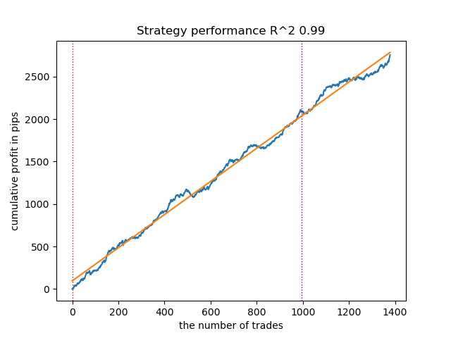
Figure 1. Testing GaussianHMM with default settings

The GMMHMM algorithm also performed well, with no noticeable changes in the quality of the models observed.

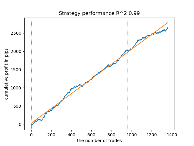
Fig. 2. Testing GMMHMM with default settings

The VariationalGaussianHMM algorithm may seem like an outlier, but after a few retrains, it can produce better curves.

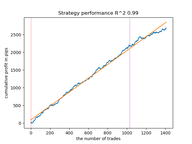
Fig. 3. Testing VariationalGaussianHMM with default settings

Overall, all algorithms have proven workable, meaning we can move on to tuning their parameters.

Increasing the number of launch iterations (n_iter = 100)

With an increase in the number of iterations of training Markov models, the results on new data improved somewhat for all modifications of the algorithm. This is apparently due to the fact that the algorithms found more favorable local optima. Overall, at this stage, no significant differences were observed in the quality of the resulting models for different algorithms. But GaussianHMM trained somewhat faster due to its simplicity.

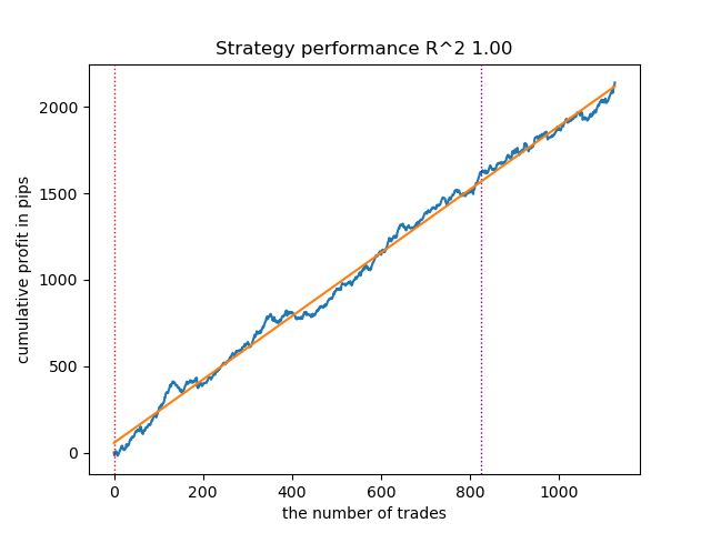
Fig. 4. Testing GaussianHMM with n_iter = 100

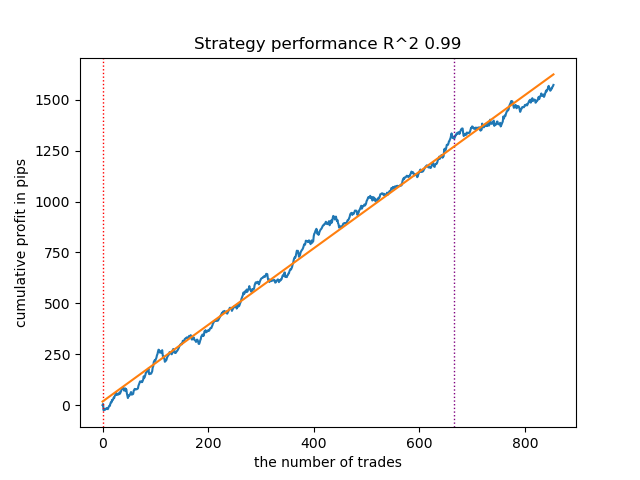
Fig. 5. Testing GMMHMM with n_iter = 100

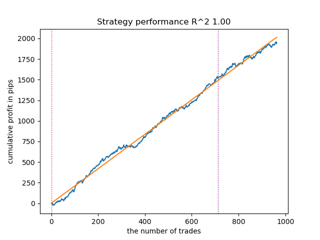
Fig. 6. Testing VariationalGaussianHMM with n_iter = 100

Reducing the number of market regimes to three

The number of iterations affects the quality of the models. Let's leave this parameter equal to 100 iterations. Let's try to reduce the number of regimes (hidden states of the models) to three and look at the results.

hyper_params = {
    'symbol': 'XAUUSD_H1',
    'export_path': '/drive_c/Program Files/MetaTrader 5/MQL5/Include/Trend following/',
    'model_number': 0,
    'markup': 0.2,
    'stop_loss':  10.000,
    'take_profit': 5.000,
    'periods': [i for i in range(5, 300, 30)],
    'periods_meta': [5],
    'backward': datetime(2000, 1, 1),
    'forward': datetime(2024, 1, 1),
    'full forward': datetime(2026, 1, 1),
    'direction': 'buy',
    'n_clusters': 3,
}

GaussianHMM, GMMHMM, and VariationalGaussianHMM performed well in identifying the three market regimes, but the last one required several training restarts.

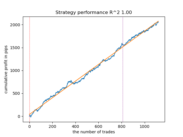
Figure 7. Testing VariationalHMM with n_iter = 100 and three regimes

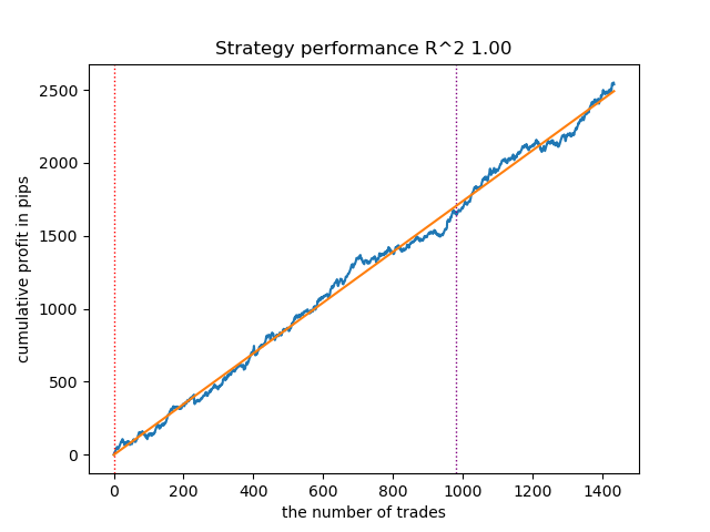
Fig. 8. Testing GMMHMM with n_iter = 100 and three regimes

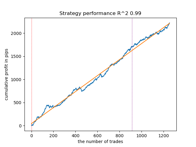
Figure 9. Testing VariationalGaussianHMM with n_iter = 100 and three regimes

Creating prior covariance matrices for hidden Markov models

In the theoretical part of the article, five methods for determining prior covariance matrices for time series were considered. The first and last methods are the most suitable for us. Let's recall them:

Empirical assessment. One of the most direct methods is to estimate the covariance matrix directly from previously collected time series data. The sample covariance matrix reflects the covariance between the different components of the time series, where each element (i, j) of the matrix represents the sample covariance between the i-th and j-th components, and the diagonal elements represent the sample variances. For the X time series of length T and dimension p, the sample covariance matrix Σ̂ can be calculated using the standard equation. However, the application of empirical estimation to time series has its limitations. First, the time series is assumed to be stationary, that is, its statistical properties, such as mean and covariance, do not change over time. Second, obtaining a reliable estimate requires a sufficient amount of data compared to the dimensionality of the time series. Third, when the sample size is small compared to the dimensionality, the covariance matrix may suffer from singularity, making it unsuitable for use in some algorithms. Despite these limitations, empirical estimation can serve as a reasonable starting point if sufficient stationary data are available.
Structural assumptions about time series. If a time series exhibits known autocorrelation properties, this knowledge can be used to generate a prior covariance matrix. For example, analyzing the autocorrelation function (ACF) and partial autocorrelation function (PACF) can help identify the order of autoregressive (AR) or moving average (MA) processes that may describe the time series. Based on the parameters of these models, it is possible to construct a prior covariance matrix reflecting known time dependencies. For example, for the AR(1) process, the structure of the covariance matrix will depend on the autocorrelation parameter. This approach assumes that the time series can be adequately described by some time series model, and that the parameters of this model can be estimated based on prior data.

However, we cannot say with certainty that financial time series can be adequately described by such simple models. Experiments have shown that such priors do not always improve the results of determining hidden Markov states. In addition, I experimented with pre-clustering using k-means to initialize the transition matrices with the obtained values. This resulted in hidden Markov models producing results similar to those in the previous paper, where market regime clustering occurred, with little or no improvement in the balance curve on the new data.

Creating priors based on clustering

The training script presents an experimental function for pre-computing priors using clustering and then training hidden Markov models.

def markov_regime_switching_prior(dataset, n_regimes: int, model_type="HMM", n_iter=100) -> pd.DataFrame:
    data = dataset[(dataset.index < hyper_params['forward']) & (dataset.index > hyper_params['backward'])].copy()
    
    # Extract meta features
    meta_X = data.loc[:, data.columns.str.contains('meta_feature')]
    
    if meta_X.shape[1] > 0:
        # Format data for HMM (requires 2D array)
        X = meta_X.values
        
        # Features normalization before training
        scaler = StandardScaler()
        X_scaled = scaler.fit_transform(X)
        
        # Calculate priors from meta_features using k-means clustering
        from sklearn.cluster import KMeans
        
        # Use k-means to cluster the data into n_regimes groups
        kmeans = KMeans(n_clusters=n_regimes, n_init=10)
        cluster_labels = kmeans.fit_predict(X_scaled)
        
        # Calculate cluster-specific means and covariances to use as priors
        prior_means = kmeans.cluster_centers_  # Shape: (n_regimes, n_features)
        
        # Calculate empirical covariance for each cluster
        from sklearn.covariance import empirical_covariance
        prior_covs = []
        
        for i in range(n_regimes):
            cluster_data = X_scaled[cluster_labels == i]
            if len(cluster_data) > 1:  # Need at least 2 points for covariance
                cluster_cov = empirical_covariance(cluster_data)
                prior_covs.append(cluster_cov)
            else:
                # Fallback to overall covariance if cluster is too small
                prior_covs.append(empirical_covariance(X_scaled))
        
        prior_covs = np.array(prior_covs)  # Shape: (n_regimes, n_features, n_features)
        
        # Calculate initial state distribution from cluster proportions
        initial_probs = np.bincount(cluster_labels, minlength=n_regimes) / len(cluster_labels)
        
        # Calculate transition matrix based on cluster sequences
        trans_mat = np.zeros((n_regimes, n_regimes))
        for t in range(1, len(cluster_labels)):
            trans_mat[cluster_labels[t-1], cluster_labels[t]] += 1
            
        # Normalize rows to get probabilities
        row_sums = trans_mat.sum(axis=1, keepdims=True)
        # Avoid division by zero
        row_sums[row_sums == 0] = 1
        trans_mat = trans_mat / row_sums
    
        # Initialize model parameters based on model type
        if model_type == "HMM":
            model_params = {
                'n_components': n_regimes,
                'covariance_type': "full",
                'n_iter': n_iter,
                'init_params': ''  # Don't use default initialization
            }
            
            from hmmlearn import hmm
            model = hmm.GaussianHMM(**model_params)
            
            # Set the model parameters directly with our k-means derived priors
            model.startprob_ = initial_probs
            model.transmat_ = trans_mat
            model.means_ = prior_means
            model.covars_ = prior_covs
            
                
        # Fit the model
        model.fit(X_scaled)
        
        # Predict the hidden states (regimes)
        hidden_states = model.predict(X_scaled)
        
        # Assign states to clusters
        data['clusters'] = hidden_states    
        return data
    
    return data

The preparation of prior distributions, using the GaussianHMM model as an example, looks like this:

Data normalization. Meta features are scaled using StandardScaler to eliminate the influence of scale on clustering results.
K-means clustering. It defines the initial parameters for hidden states (regimes). The data is clustered into n_regimes clusters. The obtained cluster labels cluster_labels are used to calculate the means prior_means (cluster centers) and covariance matrices proir_covs - the empirical covariance within clusters or the total covariance if the cluster is too small.
Calculation of initial probabilities. Initial distribution initial_probs: the proportion of points in each cluster. For example, if 30% of the data belongs to cluster 0, then initial_probs[0] = 0.3.
Transition matrix. It calculates how often one cluster follows another in time.
Then, the hidden Markov model is initialized with these priors and trained.

The remaining methods make even weaker assumptions about dependencies and were therefore not considered at all. This is probably not a complete list of possible methods for determining priors. Other methods may be used but should be based on expert judgment.

Testing hidden Markov models with prior distributions

It was noticed that the scatter of results decreased. Models became less likely to get stuck in local minima, but their diversity decreased. Also, identifying market regimes using hidden Markov models typically requires a smaller number of regimes (clusters) than k-means.

The results of testing three models with given priors are given below:

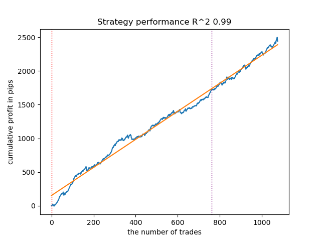
Figure 10. Testing GaussianHMM with prior distributions

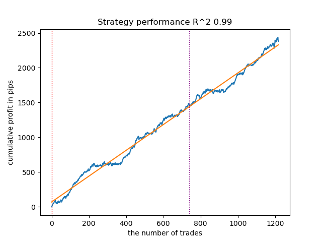
Figure 11. Testing GMMHMM with prior distributions

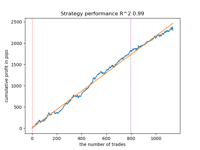
Fig. 12. Testing VariationalGaussianHMM with prior distributions

Exporting models and compiling a bot for Meta Trader 5

Exporting models occurs in exactly the same way as was suggested in previous articles. The module with export is included in the attached archive.

Let's assume that we have selected a model using a custom strategy tester.

# TESTING & EXPORT
models.sort(key=lambda x: x[0])
test_model_one_direction(models[-1][1:],
                        hyper_params['stop_loss'],
                        hyper_params['take_profit'],
                        hyper_params['forward'],
                        hyper_params['backward'],
                        hyper_params['markup'],
                        hyper_params['direction'],
                        plt=True)

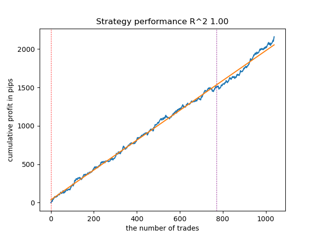
Fig. 13. Testing the best model using a custom strategy tester

Now you need to call the export function, which will save the models to the terminal folder.

export_model_to_ONNX(model = models[-1],
                     symbol = hyper_params['symbol'],
                     periods = hyper_params['periods'],
                     periods_meta = hyper_params['periods_meta'],
                     model_number = hyper_params['model_number'],
                     export_path = hyper_params['export_path'])

Then, we should compile the bot attached at the end of the article and test it in the MetaTrader 5 tester.

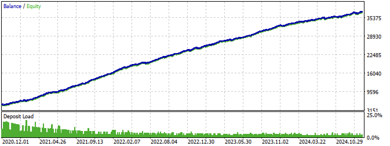
Fig. 14. Testing the best model in the Meta Trader 5 terminal for the entire period

Fig. 15. Testing the best model in the Meta Trader 5 terminal on new data

Conclusion

Hidden Markov models are an interesting method for identifying market regimes. But like all machine learning models, they are prone to overfitting on non-stationary time series.

A high-quality assignment of prior matrices allows us to find more stable market regimes that continue to remain effective on new data. Typically, fewer market regimes are required than in the case of clustering. If, in the first case, 10 clusters were needed, then in the second, it is sometimes enough to set 3-5 hidden states.

I did not find much difference in the performance of the three algorithms, they all show roughly the same results. Therefore, we can use GaussianHMM, as it is the simplest and fastest. GMMHMM, in theory, produces smoother balance curves due to the presence of a mixture of distributions, which helps identify subpatterns in each market regime, but this can lead to greater overfitting. VariationalGaussianHMM requires a more careful prior setting, while its parameters are more difficult to define and interpret.

Another useful approach might be cross-validation of models by estimating the parameters of mode distributions at different folds, but this approach was not considered in this paper.

The Python files.zip archive contains the following files for development in the Python environment:

Filename	Description
one direction HMM.py	The main script for training models
labeling_lib.py	Updated module with trade labeling module
tester_lib.py	Updated custom strategy tester based on machine learning
export_lib.py	Module for exporting models to the terminal
XAUUSD_H1.csv	The file with quotes exported from the MetaTrader 5 terminal

The MQL5 files.zip archive contains files for the MetaTrader 5 terminal:

Filename	Description
one direction HMM.ex5	The compiled bot from the article
one direction HMM.mq5	Bot source code from the article
Include//Trend following folder	The ONNX models and the header file for connecting to the bot

Translated from Russian by MetaQuotes Ltd.
Original article: https://www.mql5.com/ru/articles/17917

Attached files |

Download ZIP

Python_files.zip (548.83 KB)

MQL5_files.zip (134.83 KB)

Warning: All rights to these materials are reserved by MetaQuotes Ltd. Copying or reprinting of these materials in whole or in part is prohibited.

This article was written by a user of the site and reflects their personal views. MetaQuotes Ltd is not responsible for the accuracy of the information presented, nor for any consequences resulting from the use of the solutions, strategies or recommendations described.

dmitrievsky

Russia
41578

https://t.me/dmitrievskyai

There are two hard problems in computer science: 1) computers and 2) science.