
Exploring Regression Models for Causal Inference and Trading
Introduction
Over the course of several articles, we have explored various methods of classifying time series, but we have not touched upon regression models. Regression models, unlike binary classification, allow us to predict not the probability of an observation belonging to a particular class, but continuous values, which expands the possibilities of their application for creating automated trading systems.
Binary classification is a fundamental machine learning task in which the goal is to classify input data into one of two different categories or classes. In the context of a Forex trading bot, this usually means predicting a "buy" (represented as 0) or "sell" (represented as 1) signal. This approach reduces complex market dynamics to a simple directional decision.
The most significant inherent limitation of binary classification for quantitative trading is its inability to quantify the magnitude or intensity of a predicted price movement. A binary classifier only indicates whether the price is expected to move up or down, without providing any information about how much it is expected to change. This lack of granularity fundamentally limits decision-making in trading.
The accuracy of the classifier's predictions alone does not take into account the magnitude of change, and is therefore not very useful for trading. This aspect is key because it highlights that high directional accuracy (e.g. predicting the correct direction 70% of the time) does not automatically lead to profitable trading.
There is an important observation that high direction accuracy does not guarantee profitability. For example, you can be right 30% of the time and be profitable, or you can be right 70% of the time and be unprofitable. This demonstrates that the net result of a trading strategy is determined by the amount of profit on winning trades compared to the amount of loss on losing trades, and not simply the percentage of wins.
By treating all correct directional forecasts equally regardless of the actual price movement, the binary classification model is unable to distinguish between a small, insignificant price movement and a large, highly profitable one. This can lead to a scenario where many small winning trades are canceled out by a few large losing trades, or vice versa, resulting in an overall negative PnL despite seemingly high accuracy.
The lack of quantification of price movement means that the trading bot cannot prioritize trades with higher expected profits or avoid trades where the potential loss significantly outweighs the potential profit, even if the direction is predicted correctly. Without information about the magnitude, the bot operates with a blind spot regarding the actual financial impact of its decisions, resulting in suboptimal or even negative cumulative returns despite a high percentage of direction-based wins.
Labeling function modification
Consider the following scenario: there is a financial time series that needs to be predicted based on a set of features. In the case of binary classification, the direction of a future trade (buy or sell) can be determined, and these labels are always fixed. We cannot label them differently to obtain a more accurate estimate of the magnitude of future price deviations. The trades are equivalent regardless of how much the price actually changed.
Now imagine that we can predict not only the direction of a trade, but also the magnitude of the future change. This will allow us to fine-tune our trading system by creating additional filters that will help identify only the predicted price fluctuations that are significant for trading and exclude insignificant ones.
To train a regression model, it is necessary to prepare features and targets for its training. The features may be shared by the classifier and the regressor, while the target variables will differ.
Let's write a simple function that implements example labeling for a regression model:
@njit
def calculate_labels_r(close_data, min_val, max_val):
    labels = []
    for i in range(len(close_data) - max_val):
        rand = random.randint(min_val, max_val)
        labels.append(close_data[i + rand] - close_data[i])
    return labels

def get_labels_r(dataset, min = 1, max = 15) -> pd.DataFrame:
    # Extract closing prices from the dataset
    close_data = dataset['close'].values
    labels = calculate_labels_r(close_data, min, max)
    # Trim the dataset to match the length of calculated labels
    dataset = dataset.iloc[:len(labels)].copy()
    # Add the calculated labels as a new column
    dataset['labels'] = labels
    # Remove rows with NaN values (potentially introduced in 'calculate_labels')
    dataset = dataset.dropna()
    return dataset
The main difference from the binary classification labeling is that we now determine price changes (subtract the current price from the future price) instead of simply determining the direction (buy or sell). The code is accelerated by Numba, so target labeling is very fast.
The above function only takes into account the difference between a randomly selected future price in the range {min_val; max_val} and the current one. This may not be entirely correct, since intermediate deviations, which may be significant, are not taken into account. I propose another modification of the deviation calculation function, which is presented below.
@njit
def calculate_labels_mean_r(close_data, min_val, max_val):
    labels = []
    for i in range(len(close_data) - max_val):
        # Calculate the average price value in the window from min_val to max_val
        future_prices = close_data[i + min_val : i + max_val + 1]
        mean_future_price = np.mean(future_prices)
        # Calculate the difference between the average future value and the current price
        labels.append(mean_future_price - close_data[i])
    return labels

def get_labels_r(dataset, min = 1, max = 15) -> pd.DataFrame:
    # Extract closing prices from the dataset
    close_data = dataset['close'].values
    # Calculate buy/hold labels based on future price movements
    labels = calculate_labels_mean_r(close_data, min, max)
    # Trim the dataset to match the length of calculated labels
    dataset = dataset.iloc[:len(labels)].copy()
    # Add the calculated labels as a new column
    dataset['labels'] = labels
    # Remove rows with NaN values (potentially introduced in 'calculate_labels')
    dataset = dataset.dropna()
    return dataset
Now the function takes into account all deviations in the given interval, calculating the average value. After this, the difference between the average value of future prices and the current price is calculated. Accordingly, the get_labels_r() function now calls the calculate_labels_mean_r() labeling function, and not calculate_labels_r() as before. We can experiment by calling different labeling functions.
Adding a causal inference system
For more accurate predictions, we use an algorithm similar to the one described in the article about the causal inference. The main difference will be the use of a regressor rather than a classifier.
def meta_learners(data, models_number: int, iterations: int, depth: int):
    data = data.copy()
    data = data[(data.index < hyper_params['forward']) & (data.index > hyper_params['backward'])].copy()

    X = data[data.columns[1:-1]]
    y = data['labels']
    data['meta_labels'] = 0

    for i in range(models_number):
        X_train, X_val, y_train, y_val = train_test_split(
            X, y, train_size = 0.5, test_size = 0.5, shuffle = True)

        # fit debias model with train and validation subsets
        meta_m = CatBoostRegressor(iterations = iterations,
                                depth = depth,
                                verbose = False,
                                use_best_model = True)

        meta_m.fit(X_train, y_train, eval_set = (X_val, y_val), plot = False)

        coreset = X.copy()
        coreset['labels'] = y
        coreset['labels_pred'] = meta_m.predict(X)
        data['meta_labels'] += abs(coreset['labels'] - coreset['labels_pred'])

    data['meta_labels'] = data['meta_labels'] / models_number
    return data
The function trains multiple regressors on random subsets of data from the original dataset and then compares the actual targets with the predicted ones. Thus, the meta model will not predict 0 or 1 (trade or not trade), but the average values of deviations of forecasts from actual ones. This way we can filter out forecasts that deviate significantly from expected values.
Training and testing trained models
For testing regression models, the tester was modified. Now it features the 'r' suffix. It is time to train several models. In this article, I will train 10 models and select the one I like best.
hyper_params = {
    'symbol': 'EURUSD_H1',
    'export_path': '/Users/dmitrievsky/drive_c/Program Files/MetaTrader 5/MQL5/Include/Trend following/',
    'model_number': 0,
    'markup': 0.00010,
    'stop_loss':  0.00500,
    'take_profit': 0.00200,
    'periods': [i for i in range(5, 100, 30)],
    'backward': datetime(2010, 1, 1),
    'forward': datetime(2024, 1, 1),
}

models = []
for i in range(10):
    print('Learn ' + str(i) + ' model')
    data = get_labels_r(get_features(get_prices()), min=1, max=15)
    dataset = meta_learners(data=data, models_number=5, iterations=15, depth=3)
    models.append(fit_final_models(dataset, tol=3e-2))
Here we should pay attention to the tol parameter, which is passed to the final model training function. Since we want to make the main model as robust as possible, there is no point in training it on all examples. We will train it only on those examples whose predictions deviate from the actual ones by less than the tol value.
Since deviations from predictions are actually counted in points, then tol=3e-2 will mean a maximum difference of 0.03 or 300 4-digit points. It may seem like a large difference as a filter, but it is worth considering that this is a difference in absolute values, as predictions can be either positive or negative. You can experiment with this parameter. Below is the function itself.
def fit_final_models(dataset, tol=1e-2) -> list:
    # features for model\meta models. We learn main model only on filtered labels
    X = dataset[dataset['meta_labels'] < tol]
    X, X_meta = X[X.columns[1:-2]], dataset[dataset.columns[1:-2]]
    # labels for model\meta models
    y = dataset[dataset['meta_labels'] < tol]
    y, y_meta = y[y.columns[-2]], dataset[dataset.columns[-1]]

    # fit main model with train and validation subsets
    model = RandomForestRegressor(n_estimators=50, max_depth=10)
    model.fit(X, y)
    # fit meta model with train and validation subsets
    meta_model = RandomForestRegressor(n_estimators=50, max_depth=10)
    meta_model.fit(X_meta, y_meta)

    data = get_features(get_prices())
    R2 = test_model_r(data,
                    [model, meta_model],
                    hyper_params['stop_loss'],
                    hyper_params['take_profit'],
                    hyper_params['forward'],
                    hyper_params['backward'],
                    hyper_params['markup'],
                    plt=False)

    if math.isnan(R2):
        R2 = -1.0
        print('R2 is fixed to -1.0')
    print('R2: ' + str(R2))
    result = [R2, model, meta_model]
    return result
Now let's sort the models and call the custom tester function:
models.sort(key=lambda x: x[0])
data = get_features(get_prices())
test_model_r(data,
        models[-1][1:],
        hyper_params['stop_loss'],
        hyper_params['take_profit'],
        hyper_params['forward'],
        hyper_params['backward'],
        hyper_params['markup'],
        plt=True)
The model is overfitted and performs poorly on new data:
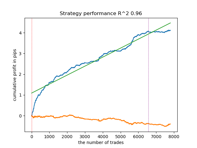
Fig. 1. Testing the model with basic labeling
We will carry out exactly the same manipulations, but we will use the calculate_labels_mean_r() trade-labeling function, which calculates average future prices.
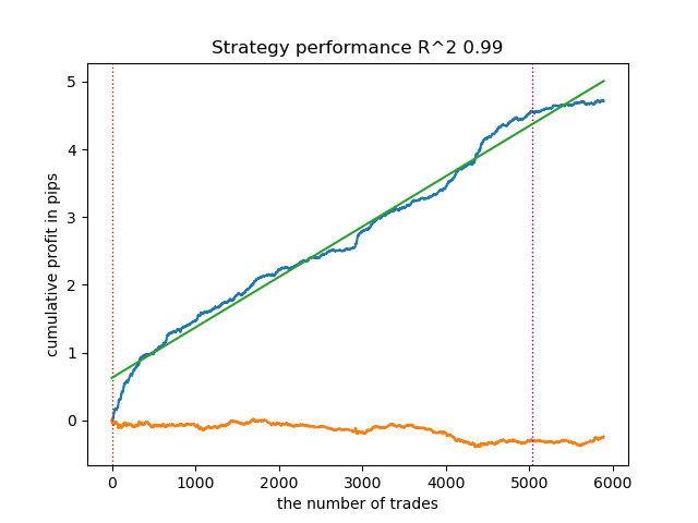
Fig. 2. Testing the model with averaged labeling
The second trade-labeling function, on average, shows more stable results on new data. Apparently this is due to the fact that the average value of future prices is taken into account.
The custom tester does not have the ability to define thresholds for the main regression model, so it simply divides the model predictions into positive and negative, meaning the signals are still quite rough. But we will fix this directly in the MetaTrader 5 terminal.
Exporting models to the MetaTrader 5 terminal
Now we need to export the models to the terminal in ONNX format and configure the trading system. The export function looks familiar:
export_model_to_ONNX(model = models[-1],
                     symbol = hyper_params['symbol'],
                     periods = hyper_params['periods'],
                     periods_meta = hyper_params['periods'],
                     model_number = hyper_params['model_number'],
                     export_path = hyper_params['export_path'])
It should be noted that I was unable to use CatBoost regression models in ONNX format with the terminal, so I used Random Forest instead.
The dimension of the input tensor is adjusted automatically depending on the hyperparameters (number of features) that are specified before training begins. Next, the models are converted to ONNX format using the convert_sklearn() function and saved to disk in the directory you specified in the hyperparameters.
def export_model_to_ONNX(**kwargs):
    model = kwargs.get('model')
    symbol = kwargs.get('symbol')
    periods = kwargs.get('periods')
    periods_meta = kwargs.get('periods_meta')
    model_number = kwargs.get('model_number')
    export_path = kwargs.get('export_path')

    initial_type = [('float_input', FloatTensorType([None, len(hyper_params['periods'])]))]
    onnx_model = convert_sklearn(model[1], initial_types=initial_type)
    # save main model to ONNX
    with open(export_path +'catmodel ' + symbol + ' ' + str(model_number) +'.onnx', "wb") as f:
        f.write(onnx_model.SerializeToString())
    onnx_model_meta = convert_sklearn(model[2], initial_types=initial_type)
    # save meta model to ONNX
    with open(export_path +'catmodel_m ' + symbol + ' ' + str(model_number) +'.onnx', "wb") as f:
        f.write(onnx_model_meta.SerializeToString())

    code = '#include <Math\Stat\Math.mqh>'
    code += '\n'
    code += '#resource "catmodel '+ symbol + ' '+str(model_number)+'.onnx" as uchar ExtModel_' + symbol + '_' + str(model_number) + '[]'
    code += '\n'
    code += '#resource "catmodel_m '+ symbol + ' '+str(model_number)+'.onnx" as uchar ExtModel2_' + symbol + '_' + str(model_number) + '[]'
    code += '\n\n'
    code += 'int Periods' + symbol + '_' + str(model_number) + '[' + str(len(periods)) + \
        '] = {' + ','.join(map(str, periods)) + '};'
    code += '\n'
    code += 'int Periods_m' + symbol + '_' + str(model_number) + '[' + str(len(periods_meta)) + \
        '] = {' + ','.join(map(str, periods_meta)) + '};'
    code += '\n\n'

    # get features
    code += 'void fill_arays' + symbol + '_' + str(model_number) + '( double &features[]) {\n'
    code += '   double pr[], ret[];\n'
    code += '   ArrayResize(ret, 1);\n'
    code += '   for(int i=ArraySize(Periods'+ symbol + '_' + str(model_number) + ')-1; i>=0; i--) {\n'
    code += '       CopyClose(NULL,PERIOD_H1,1,Periods' + symbol + '_' + str(model_number) + '[i],pr);\n'
    code += '       ret[0] = MathStandardDeviation(pr);\n'
    code += '       ArrayInsert(features, ret, ArraySize(features), 0, WHOLE_ARRAY); }\n'
    code += '   ArraySetAsSeries(features, true);\n'
    code += '}\n\n'

    # get features
    code += 'void fill_arays_m' + symbol + '_' + str(model_number) + '( double &features[]) {\n'
    code += '   double pr[], ret[];\n'
    code += '   ArrayResize(ret, 1);\n'
    code += '   for(int i=ArraySize(Periods_m' + symbol + '_' + str(model_number) + ')-1; i>=0; i--) {\n'
    code += '       CopyClose(NULL,PERIOD_H1,1,Periods_m' + symbol + '_' + str(model_number) + '[i],pr);\n'
    code += '       ret[0] = MathStandardDeviation(pr);\n'
    code += '       ArrayInsert(features, ret, ArraySize(features), 0, WHOLE_ARRAY); }\n'
    code += '   ArraySetAsSeries(features, true);\n'
    code += '}\n\n'

    file = open(export_path + str(symbol) + ' ONNX include' + ' ' + str(model_number) + '.mqh', "w")
    file.write(code)

    file.close()
    print('The file ' + 'ONNX include' + '.mqh ' + 'has been written to disk')
Setting thresholds in the MetaTrader 5 terminal
Now that we have two regression models instead of two classifiers, we have the ability to set specific numerical thresholds.
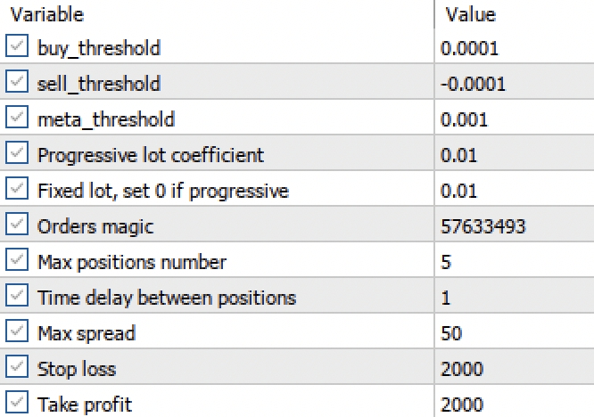
Fig. 3. Setting up signal activation thresholds in the terminal
- The buy_threshhold and sell_threshhold are responsible for filtering the signals of the main regression model. If the signal is below this threshold, no trades are opened. For example, if the predicted price change is less than 10 pips, then opening such a trade does not make much sense, since it will not cover the spread and commission.
- The meta_threshhold filters the signals of the main model based on the causal inference described earlier. It tests how much the forecast is likely to differ from the future actual change. If the difference is too big, then the trades will not be opened either.
Now let's test our model in the MetaTrader 5 tester with the given thresholds:
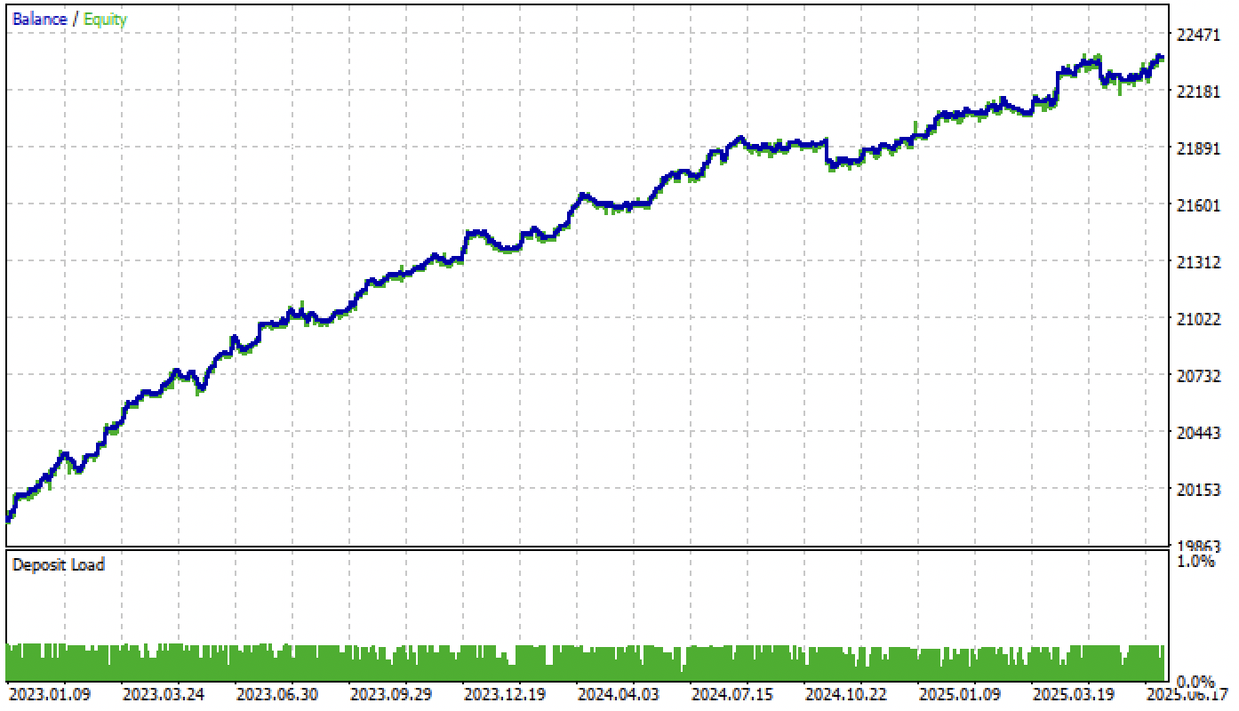
Fig. 4. Testing a model with given thresholds
Let me remind you that the forward period starts at the beginning of 2024 and the model now handles this forward period quite steadily. This highlights the importance of properly defining and setting thresholds. You can optimize the threshold values yourself.
The variety of models can be large, depending on the type of features (in this article, both models are trained on standard deviations) and on the model parameters themselves. For example, another model was trained with different parameters, which performed well on new data even without adjusting the thresholds.
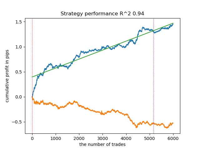
Fig. 5. Training and testing a different model with different training parameters
After adjusting the thresholds, the model showed steady growth from the beginning of 2024.
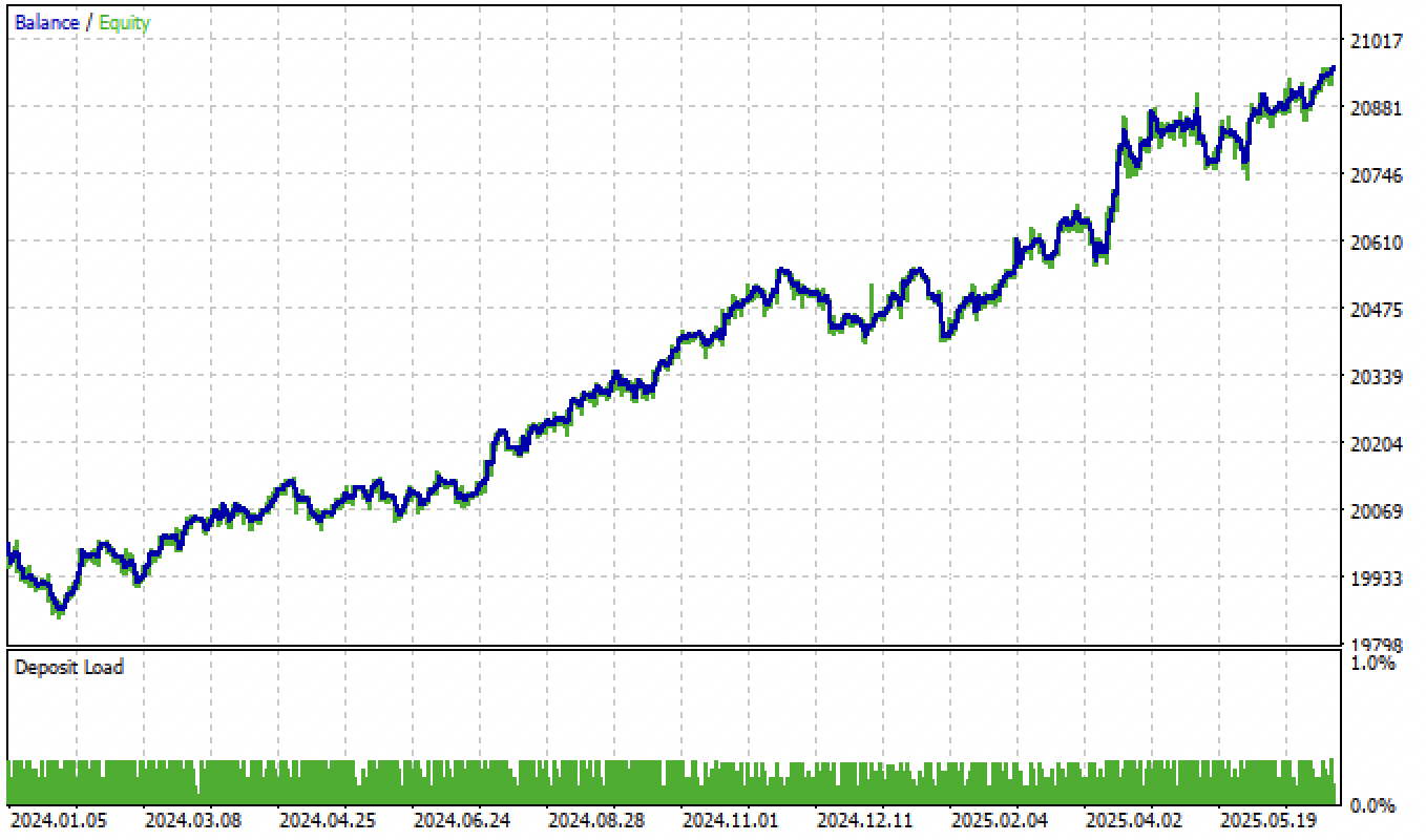
Fig. 6. Testing the model in the terminal after setting the thresholds
Testing models based on a second trade-labeling function and filtering by thresholds yields even more interesting and accurate results:

Fig. 7. Testing the model based on the average trade-labeling function and tol = 1e-2
If we change the tol parameter when training from 1e-2 to 1e-3, the results will be even better:
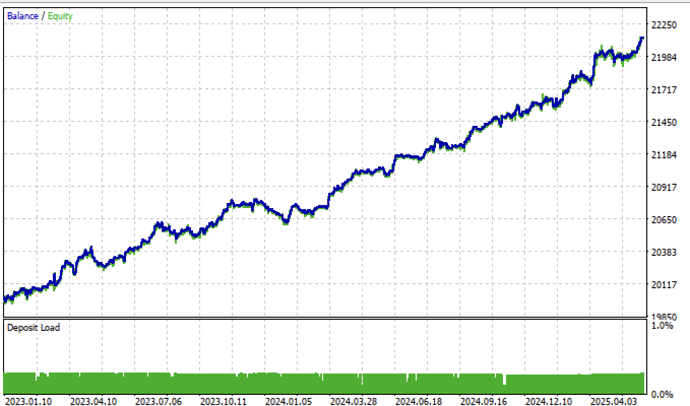
Fig. 8. Testing the model based on the average trade-labeling function and tol = 1e-3
Additional information
To export models, we need to install and import the skl2onnx package:
from skl2onnx import convert_sklearn
from skl2onnx.common.data_types import FloatTensorType
The ONNX model launch code in the trading bot code has also been modified to correctly handle new regression models:
vectorf y_main(1), y_meta(1);

OnnxRun(ExtHandle, ONNX_DEBUG_LOGS, f, y_main);
OnnxRun(ExtHandle2, ONNX_DEBUG_LOGS, f_m, y_meta);

float sig = y_main[0];
float meta_sig = y_meta[0];
Added new input variables for adjusting and optimizing thresholds:
input double buy_threshold = 0.00001;
input double sell_threshold = -0.00001;
input double meta_threshold = 0.001;
ONNX model names are now accessed via #define directives, making it easier to include models with different names:
#define model ExtModel_EURUSD_H1_0
#define model_m ExtModel2_EURUSD_H1_0
#define periods PeriodsEURUSD_H1_0
#define periods_m Periods_mEURUSD_H1_0
#define fill_arrays fill_araysEURUSD_H1_0
#define fill_arrays_m fill_arays_mEURUSD_H1_0
Trading signals are generated when conditions are triggered depending on the thresholds:
if((Ask-Bid < max_spread*_Point) && MathAbs(meta_sig) < meta_threshold &&
      AllowTrade(OrderMagic))
      if(countOrders(OrderMagic) < max_orders &&
         CheckMoneyForTrade(_Symbol, LotsOptimized(), ORDER_TYPE_BUY))
        {
         double l = LotsOptimized();
         if(sig > buy_threshold && Allow_Buy)
           {
            int res = -1;
            do
              {
               double stop = Bid - stoploss * _Point;
               double take = Ask + takeprofit * _Point;
               res = mytrade.PositionOpen(_Symbol, ORDER_TYPE_BUY, l, Ask, stop, take, bot_comment);
               Sleep(50);
              }
            while(res == -1);
           }
         else
           {
            if(sig < sell_threshold && Allow_Sell)
              {
               int res = -1;
               do
                 {
                  double stop = Ask + stoploss * _Point;
                  double take = Bid - takeprofit * _Point;
                  res = mytrade.PositionOpen(_Symbol, ORDER_TYPE_SELL, l, Bid, stop, take, bot_comment);
                  Sleep(50);
                 }
               while(res == -1);
              }
           }
        }
The modified strategy tester and model export function have been added to the corresponding modules and attached to the article.
Conclusion
In this article, I described a possible, but not the only, way to build trading systems based on regression models. This approach allows for more fine-tuning of machine learning-based bots. It also allows turning obviously unprofitable models into profitable ones by setting thresholds. You can use any features and/or trade-labeling functions, and also test this algorithm on other trading instruments and other timeframes.
The Python files.zip archive contains the following files for development in the Python environment:
| Filename | Description |
|---|---|
| causal regression.py | The main script for training models |
| labeling_lib.py | Updated trade-labeling module |
| tester_lib.py | Updated custom strategy tester based on machine learning |
| export_lib.py | Module for exporting models to the terminal |
| EURUSD_H1.csv | Quote data exported from MetaTrader 5 |
The MQL5 files.zip archive contains files for the MetaTrader 5 terminal:
| Filename | Description |
|---|---|
| regression trader.ex5 | The compiled bot from the article |
| regression trader.mq5 | Bot source code from the article |
| Include//Trend following folder | The ONNX models and the header file for connecting to the bot |
Translated from Russian by MetaQuotes Ltd.
Original article: https://www.mql5.com/ru/articles/18603
Warning: All rights to these materials are reserved by MetaQuotes Ltd. Copying or reprinting of these materials in whole or in part is prohibited.
This article was written by a user of the site and reflects their personal views. MetaQuotes Ltd is not responsible for the accuracy of the information presented, nor for any consequences resulting from the use of the solutions, strategies or recommendations described.
- Free trading apps
- Over 8,000 signals for copying
- Economic news for exploring financial markets
You agree to website policy and terms of use
I use causal_regression_orig.py to produce ea header file, then compile ea.
The result is test_result pic in below.
There are so less trades than the one you posted.
So what's the difference between these.
Are there a lot of trades in python tester? If yes, you need to reconfigure the thresholds for opening trades in mql5 programme, maybe they are too big.
This is the python tester result, I use the same code as you attached in this post. I checked in mt5 tester config panel, the buy_threshold and sell_threshold are both 0.0001 and -0.0001, same as the setting in this post.
I checked the code, and didnot know what is the difference between this.
This is the python tester result, I use the same code as you attached in this post. I checked in mt5 tester config panel, the buy_threshold and sell_threshold are both 0.0001 and -0.0001, same as the setting in this post.
I checked the code, and didnot know what is the difference between this.
Greetings Maxim, thank you very much for sharing with us.
Question. After calculating ONNX for a new ticker and placing it in the Trend Following folder, how can I make sure that the EA starts using the trained data for the new ticker? For other tickers, even if I delete ONNX_EURUSD and place another one, the EA behaves identically. Do I need to change something in MQL5 Expert Advisor when changing the ticker?
Greetings Maxim, thank you so much for sharing with us.
Question. After calculating ONNX for a new ticker and placing it in the Trend Following folder, how can I make sure that the EA starts using the trained data for the new ticker? For other tickers, even if I delete ONNX_EURUSD and place another one, the EA behaves identically. Do I need to change something in MQL5 Expert Advisor when changing the ticker?
Hi, you need to connect the .mqh file with the new ticker in the EA code.
That is, change the selected one to another file with a different name, which was generated by the python script.