Neural Networks in Trading: A Cross-Domain Time Series Forecasting Framework (Conclusion)

Introduction

Over the past few decades, financial trading has undergone fundamental changes, evolving into a high-tech and highly disciplined field. Whereas a trader’s success used to depend largely on intuition, experience, and personal observations, today the ability to process vast amounts of data quickly and effectively, generate accurate forecasts, and make decisions based on advanced algorithms has come to the forefront. With the advancement of computing power and the emergence of modern machine learning methods, traders and researchers now have new tools capable of identifying patterns and trends in the apparent chaos of market data. Nevertheless, despite significant progress, short- and medium-term forecasting of financial market time series remains a highly complex task.

The reason lies in the unique and complex nature of financial markets. Financial markets are highly noisy systems — where true signals are often obscured by a mass of random fluctuations and artifacts. Market data are non-stationary: their statistical properties change over time, which manifests itself in shifts between market regimes — from calm phases to volatile ones and back again. In addition, markets are subject to sudden events — such as news, crises, or regulatory interventions — that disrupt normal price patterns. All of this creates an environment in which traditional time-series models face fundamental limitations.

Classical statistical methods have proven effective in the analysis of stationary processes; however, their applicability to modern market data is limited. On the other hand, neural networks — including LSTM and GRU — have become widely used as more flexible tools for modeling complex temporal dependencies. However, they also require large amounts of data for training, and when transitioning to new assets or market conditions, they often lose accuracy and stability. The reason is that most models are tied to specific data structures and patterns, which are not always universal.

In this regard, a key challenge arises: how to build a model capable of generalization and adaptation without additional training, known as Zero-Shot Forecasting. Such a model, trained on a large number of diverse time series from various domains, should have an internal representation that allows it to recognize similar patterns and regularities in completely new, previously unseen data. This fundamentally changes the approach to forecasting: the model is no longer a specialist in a single market but becomes a versatile analyst capable of transferring knowledge across different tasks.

The TimeFound framework, which we began exploring in the previous article, was developed specifically for this concept. TimeFound is a powerful and versatile cross-domain time series model based on the Transformer architecture. Transformer, a revolutionary method first proposed for natural language processing tasks, has become widely adopted due to its ability to effectively capture long-range dependencies in sequences. In TimeFound, this potential is used to analyze financial time series, but with an important addition: the Multi-Resolution Patching mechanism.

The idea behind Multi-Resolution Patching is to divide the original time series into patches — segments of varying lengths that reflect different time scales. For example, short patches capture local and rapid fluctuations, while longer ones capture slower, more global trends. This multi-level approach allows the model to simultaneously account for multiple layers of information, which is critically important for financial data, where signals emerge across different time horizons.

From a technical standpoint, the TimeFound architecture consists of a set of independent projection modules — one for each group of patches of a specific scale. Each such module consists of a small two-layer perceptron with residual connections. It takes patches and binary masks of valid points as input, which helps it effectively ignore padding and artificially filled missing values. Thanks to separate projection modules and the specifics of patch repetition, the model distinguishes the contribution of each time scale, which provides robustness to phase shifts, variations in the length of the input data, and missing values.

To train TimeFound, an extensive dataset of time series from a wide variety of fields — ranging from macroeconomic indicators and market quotes to physical processes — was collected and carefully prepared. This enabled the model to develop the ability to generalize and perform well on new, previously unseen data.

A custom visualization of the framework is shown below.

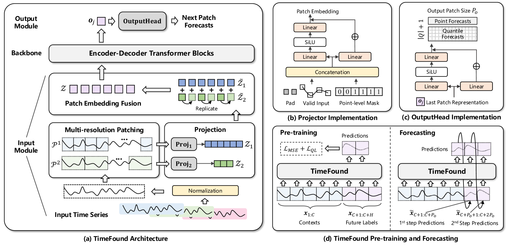
In the practical section of the previous article, we took a detailed look at the implementation of the multi-scale patching module — a key component of the TimeFound framework’s data preparation block. This module is responsible for efficiently generating informative tokens — compact, information-rich representations of individual fragments of a time series, split into patches of varying lengths and scales. It is precisely thanks to this mechanism that the model is able to perceive and process data while taking into account both local and global market characteristics.

Today we will continue the work we started.

TimeFound Encoder–Decoder

The token tensor, which is formed during the patching stage, is passed to the Transformer block for further analysis. This is where intelligent data processing begins — identifying hidden patterns, forecasting dynamics, and generating signals.

The authors of the TimeFound framework suggest using the classic Encoder–Decoder architecture in this part of the architecture, which is well known from machine translation and sequence analysis models. However, in the context of time series, this scheme was adapted and enhanced with a number of additions to account for the specific characteristics of the data.

The Encoder uses bidirectional Self-Attention. This means that each token is analyzed in the context of all the others, both forward and backward along the timeline. Thus, the model can take into account not only what happened up to the current moment, but also potential dependencies on events that occur later. This is particularly useful when analyzing already completed segments of historical data. This approach makes it possible to identify deeper interrelationships.

In the Decoder, on the other hand, visibility is intentionally limited: each token can see only those that precede it in time. A key component of the Decoder is the cross-attention (Cross-Attention) module. Here, the data received from the Encoder are provided as context, and the Decoder correlates the input tokens with this contextual information. This allows for more accurate output predictions.

This division of tasks between the Encoder and the Decoder, along with the use of attention mechanisms, makes the TimeFound architecture particularly flexible. It is capable not only of reacting to recent price movements, but also of analyzing an asset’s behavior within a broad historical context, taking market patterns into account, and distinguishing between ordinary noise and meaningful signals.

Our library already includes a wide range of variations of Self- and Cross-Attention modules — from basic ones to more advanced versions with masking and dynamic selection of attention heads. And, of course, we will not pass up the opportunity to build on this prior work as part of implementing the TimeFound model. However, it is important to note one conceptual nuance here: the authors of the framework propose using an autoregressive approach to generate a forecast.

The model does not generate a forecast for the entire time period in a single step. Instead, it operates iteratively. At each iteration, the Transformer takes historical data as input — a tensor of tokens representing various scales of market patterns — and generates a single token that corresponds to the next segment. This token is interpreted as a forecast state. The result is added to the historical data, and the process is repeated. Thus, the forecast is built step by step over the entire horizon of interest.

In our case, we do not aim to make forecasts far into the future. We are not engaging in fortune-telling; instead, we are building a systematic position-management algorithm. The model runs on each new bar, recalculates the state based on actual, already known data, and outputs a decision: hold, close, reverse the position, or increase the position size. Of course, when executing a trade, we make a forecast over a certain horizon, but on each new bar we adjust it in line with the updated reality.

Nevertheless, the very principle of autoregression imposes certain architectural requirements. At each step, the same set of historical data must be fed into both the Encoder and the Decoder. The Encoder analyzes these data in the context of the entire history, identifying general patterns, while the Decoder uses the current state — which is part of the same historical sequence — to analyze it in the context of the historical dependencies identified by the Encoder and to generate forecast values. Thus, we obtain two parallel processing streams operating on the same data.

To ensure this synchronization, we will create a CNeuronTimeFoundTransformerUnit object. Its purpose is to manage the flow of information centrally. This will help maintain a clean architecture and simplify future scaling or component replacement. The structure of the new object is shown below.

class CNeuronTimeFoundTransformerUnit  :  public CNeuronCrossDMHAttention
  {
protected:
   CNeuronMVMHAttentionMLKV   cSelfAttention;
   //---
   virtual bool      feedForward(CNeuronBaseOCL *NeuronOCL) override;
   virtual bool      feedForward(CNeuronBaseOCL *NeuronOCL, CBufferFloat *SecondInput) override
                                                              { return feedForward(NeuronOCL); }
   virtual bool      calcInputGradients(CNeuronBaseOCL *prevLayer) override;
   virtual bool      calcInputGradients(CNeuronBaseOCL *NeuronOCL, CBufferFloat *SecondInput,
                                        CBufferFloat *SecondGradient, ENUM_ACTIVATION SecondActivation = None)
                                        override
                                        { return calcInputGradients(NeuronOCL); }
   virtual bool      updateInputWeights(CNeuronBaseOCL *NeuronOCL) override;
   virtual bool      updateInputWeights(CNeuronBaseOCL *NeuronOCL, CBufferFloat *SecondInput) override
                                        { return updateInputWeights(NeuronOCL); }

public:
                     CNeuronTimeFoundTransformerUnit(void) {};
                    ~CNeuronTimeFoundTransformerUnit(void) {};
   //---
   virtual bool      Init(uint numOutputs, uint myIndex, COpenCLMy *open_cl, uint window,
                          uint window_key, uint heads, uint heads_kv, uint units_count,
                          uint layers, uint layers_to_one_kv, uint variables,
                          ENUM_OPTIMIZATION optimization_type, uint batch);
   //---
   virtual int       Type(void) override const { return defNeuronTimeFoundTransformerUnit; }
   //---
   virtual bool      Save(int const file_handle) override;
   virtual bool      Load(int const file_handle) override;
   virtual bool      WeightsUpdate(CNeuronBaseOCL *source, float tau) override;
   virtual void      SetOpenCL(COpenCLMy *obj) override;
  }; 

In the presented structure of the new class, we see only one internal object — the Self-Attention module, which serves as the Encoder for the model being created. The functionality of the Decoder is implemented using the parent class, which is a cross-attention module.

However, behind its apparent simplicity lies a carefully designed algorithm. The role of the Encoder is fulfilled by the independent channel analysis block CNeuronMVMHAttentionMLKV. Its key feature is its ability to perform an independent analysis of each univariate sequence — that is, each variable or indicator — separately. If, for example, prices, volumes, and volatility are fed into the model, CNeuronMVMHAttentionMLKV establishes causal relationships within each time series without mixing signals at an early stage. This minimizes cross-signal noise and allows the model to better understand the structure of each data source, significantly improving the interpretability of the results obtained.

Additional efficiency comes from using the Multi-Layer Key-Value (MLKV) mechanism — one of the most elegant ideas for optimizing the computational complexity of Transformer. In classical implementations, each Self-Attention layer uses its own Key and Value. Here, however, these tensors are stored and reused across multiple layers, while Query is refined at each level. This approach reduces the computational load and at the same time allows representations to be refined progressively — as if we were rereading a familiar text, noticing new details each time. This is especially valuable in trading: on the first pass, the model can identify local patterns, and then recognize increasingly general market structures.

Thus, in this implementation, the Encoder serves a dual purpose:

1. On the one hand, classic Bi-Directional Self-Attention identifies relationships between tokens in both directions along the timeline.
2. On the other hand, it provides modular analysis of each univariate sequence, enabling a multilayered understanding of its structure.

Now let's move on to the Decoder. In this section, we use the CNeuronCrossDMHAttention module, which implements diversified multi-head cross-attention. It also offers a number of architectural advantages.

First, the Decoder, in accordance with the standard Transformer architecture, includes two types of attention modules:

• Self-Attention — analyzes the relationships between tokens in the main data stream;
• Cross-Attention — enriches these tokens with context obtained from the Encoder.

In both cases, relative positional encoding modules are used. This means that the attention block takes into account not only the token's absolute position, but also its relative position with respect to other tokens. Furthermore, this attention mechanism is supplemented by three types of biases:

• a content-dependent positional bias,
• a global context bias,
• a global positional bias.

This allows the model to more accurately account not only for the distances between events, but also for the qualitative relationships between them — which is critical for analyzing sequential market data.

Following the attention module is the multi-head FeedForward block. Its purpose is to perform independent nonlinear processing in various feature subspaces. This makes it possible to identify a wide range of market patterns without losing sight of important structural elements of the sequence.

It is also worth noting an important distinction between the components of the architecture. Unlike the Encoder, the Decoder does not separate univariate sequences. While in the Encoder each variable is analyzed in isolation, preserving independent univariate sequences, in the Decoder all tokens are combined into a single stream. At this point, there are no longer any boundaries between the univariate series — the model perceives them as a single entity.

As a result, the Decoder can analyze cross-domain dependencies. That is, relationships between variables that might not be obvious when considered separately. Price may be explained not only by its own history, but also by volatility, volume, or, say, news-flow activity. All these dependencies begin to emerge precisely in the cross-attention blocks, where current-state tokens are enriched with information encoded by the Encoder.

The result is a powerful, interpretable architecture in which the compact and elegant Encoder module CNeuronMVMHAttentionMLKV is combined with a flexible and adaptive Decoder based on CNeuronCrossDMHAttention. This model scales well, is suitable for various types of market data, and maintains high computational efficiency.

The Encoder is declared statically, which allows us to leave the class constructor and destructor empty. Inherited and declared components are initialized centrally in the Init method. The method parameters provide a set of constants that allow us to unambiguously interpret the architecture of the object being created.

bool CNeuronTimeFoundTransformerUnit::Init(uint numOutputs, uint myIndex, COpenCLMy *open_cl, uint window,
                                           uint window_key, uint heads, uint heads_kv, uint units_count,
                                           uint layers, uint layers_to_one_kv, uint variables,
                                           ENUM_OPTIMIZATION optimization_type, uint batch)
  {
   if(!CNeuronCrossDMHAttention::Init(numOutputs, myIndex, open_cl, window, window_key, variables, window,
                                      units_count * variables, heads, layers, optimization_type, batch))
      return false;
   SetActivationFunction(None);

In the method body, we first call the identically named method of the parent class, which already implements the algorithm for initializing inherited objects and interfaces.

Here, it is worth taking a closer look at the initialization parameters passed to the parent class method. First of all, it should be noted that the parent object, unlike the one we are creating, requires two streams of input data: the data being analyzed and the context. However, we plan to receive only one stream at the object's input. The context is formed by the Encoder within the module.

Furthermore, a multimodal sequence of tokens describing the historical data window under analysis is passed to the object as input data. Each univariate sequence is represented by a series of tokens, where each token corresponds to a single patch — a local segment of the time series. These patches allow the model to focus on local changes and patterns, identifying short-term dependencies within each variable.

The output of the object is expected to contain only one token for each univariate sequence, each representing the encoded prediction of the next segment of the analyzed multimodal time series. At the same time, the Transformer architecture is designed to preserve the dimensions of the main information flow.

In light of the above, we decided to feed only the tokens describing the last segment of the environment state into the main path of the Decoder: one for each univariate sequence. At the same time, all the information received, enriched with internal dependencies in the Encoder, is passed through an additional information flow.

After successfully executing the parent class method, we proceed to initialize the Encoder. Here, we provide information about the total length of the sequence being analyzed.

   if(!cSelfAttention.Init(0, 0, OpenCL, window, window_key, heads, heads_kv, units_count, layers, layers_to_one_kv,
                           variables, optimization, iBatch))
      return false;
   cSelfAttention.SetActivationFunction(None);
//---
   return true;
  }

Please note that the Encoder and the Decoder in our implementation use objects with a multi-layer architecture. We use the same number of layers in both modules.

The next step in our work is to develop a forward pass algorithm for our object. The algorithm is quite simple — we only need to call the corresponding methods, first on the Encoder and then on the Decoder. However, it is important to pay attention to certain nuances of the information flows. In the method parameters, we receive a pointer to the source data object. In it, we expect to receive data in the form of a three-dimensional tensor [Series Length × Variable × Token Size]. This is exactly the data ordering we need for the Encoder, and we immediately pass it a pointer to the object.

bool CNeuronTimeFoundTransformerUnit::feedForward(CNeuronBaseOCL *NeuronOCL)
  {
   if(!cSelfAttention.FeedForward(NeuronOCL))
      return false;

We agreed to use the tokens of the segment containing the latest environment state as the input data for the main information flow of the Decoder. But we know that the analyzed data are fed into the model in reverse chronological order: the most recent data come first. Therefore, the tokens we need are located at the beginning of the source data buffer. Taking advantage of this circumstance, we skip the step of copying the required data fragment and simply pass a pointer to the source data object through the main information flow, and the output of the Encoder through the auxiliary flow.

   if(!CNeuronCrossDMHAttention::feedForward(NeuronOCL, cSelfAttention.getOutput()))
      return false;
//---
   return true;
  }

We then complete the method, first returning the Boolean result of the operations to the calling program.

I suggest that you review the algorithms for the backward pass methods on your own. The complete source code for the CNeuronCrossDMHAttention class and all of its methods is provided in the attachment.

Model Architecture

Once we have created all the necessary objects that make up the structural components of our model, we move on to the next stage — building a cohesive architecture. It is important to note here that, as in our previous developments, we are creating a trading Agent that operates within the framework of reinforcement learning.

In the context of the task at hand, the TimeFound framework serves only to analyze the environment state — preprocessing market data and identifying hidden patterns in historical time series. It is in this role that the corresponding component will be integrated into the Environment Encoder architecture, which provides the rest of the model with a structured, cleaned, and interpretable representation of the current market situation.

Within the overall trading Agent, we follow the Actor–Director–Critic structure, in which each component performs a strictly defined task. In its current implementation, the system consists of four standalone models that work together:

• Environment State Encoder (Encoder) is responsible for in-depth analysis of incoming market data. It identifies stable patterns in the time series being analyzed, creating a rich representation of the current trading context. This representation is then passed on to the Actor.
• Actor (Actor) is the central element of the Agent. Based on the input data it receives from the Encoder, it generates specific trading decisions.
• Director (Director) and Critic (Critic) are evaluation subsystems. They evaluate the decisions made by the Actor using an internal model of the future and predict possible consequences. Moreover, the Director provides a more stringent binary assessment — whether such behavior is worth considering at all — while the Critic provides a quantitative metric of the expected reward. Together, they generate the feedback signal necessary for the Agent to learn and adapt to changing market conditions.

This approach ensures the system's modularity and flexibility: each component can be independently improved or adapted to a specific class of trading strategies.

The architecture of all models is defined in the CreateDescriptions method, which takes pointers to four dynamic arrays (one for each model) as parameters. Each of them will store a unique sequence of objects that provides a complete representation of the model being created.

bool CreateDescriptions(CArrayObj *&encoder,
                        CArrayObj *&actor,
                        CArrayObj *&director,
                        CArrayObj *&critic
                       )
  {
//---
   CLayerDescription *descr;
//---
   if(!encoder)
     {
      encoder = new CArrayObj();
      if(!encoder)
         return false;
     }
   if(!actor)
     {
      actor = new CArrayObj();
      if(!actor)
         return false;
     }
   if(!director)
     {
      director = new CArrayObj();
      if(!director)
         return false;
     }
   if(!critic)
     {
      critic = new CArrayObj();
      if(!critic)
         return false;
     }

Let's start with the Encoder. We plan to feed a tensor containing the time-series history into the model and immediately pass its data to a fully connected layer of sufficient dimensionality. This layer serves as a sort of gate for the model. We set the number of neurons equal to the product of the number of historical bars and the number of descriptors for each bar, which allows us to preserve all information about price dynamics, volumes, and other indicators.

//--- Encoder
   encoder.Clear();
//--- Input layer
   if(!(descr = new CLayerDescription()))
      return false;
   descr.type = defNeuronBaseOCL;
   int prev_count = descr.count = (HistoryBars * BarDescr);
   descr.activation = None;
   descr.optimization = ADAM;
   if(!encoder.Add(descr))
     {
      delete descr;
      return false;
     }

Next is the BatchNormWithNoise layer. It is designed to stabilize the training process and introduce a small stochastic component, which helps the model avoid getting stuck in local minima during optimization. This is where we introduce noise control: during the normalization process, random fluctuations are added, ensuring better generalization performance on real-world market data, which is often noisy.

//--- layer 1
   if(!(descr = new CLayerDescription()))
      return false;
   descr.type = defNeuronBatchNormWithNoise;
   descr.count = prev_count;
   descr.batch = BatchSize;
   descr.activation = None;
   descr.optimization = ADAM;
   if(!encoder.Add(descr))
     {
      delete descr;
      return false;
     }

After normalizing the data, let's add some information about its dynamics using the ConcatDiff module. This layer calculates first differences along the time axis and adds them to the original data as new channels, allowing the model to better capture the rates of change in the indicators.

//--- layer 2
   if(!(descr = new CLayerDescription()))
      return false;
   descr.type = defNeuronConcatDiff;
   prev_count = descr.count = HistoryBars;
   descr.layers = BarDescr;
   descr.step = 1;
   descr.batch = BatchSize;
   descr.optimization = ADAM;
   descr.activation = None;
   if(!encoder.Add(descr))
     {
      delete descr;
      return false;
     }

Next comes Mamba4CastEmbedding — here we introduce temporal encoding for each historical bar. We specify harmonics of two periodicities — hourly and daily — so that the model captures daily patterns and intraday fluctuations. After that, the embeddings for each bar are combined into an overall representation.

//--- layer 3
   if(!(descr = new CLayerDescription()))
      return false;
   descr.type = defMamba4CastEmbeding;
   prev_count = descr.count = HistoryBars;
   descr.window = 2 * BarDescr;
   int prev_out = descr.window_out = NSkills;
     {
      int temp[] = {PeriodSeconds(PERIOD_H1), PeriodSeconds(PERIOD_D1)};
      if(ArrayCopy(descr.windows, temp) < (int)temp.Size())
         return false;
     }
   descr.batch = BatchSize;
   descr.optimization = ADAM;
   descr.activation = None;
   if(!encoder.Add(descr))
     {
      delete descr;
      return false;
     }

Once the embedding is ready, we move on to TimeFoundPatching. The module divides the resulting tensor into a predetermined number of equal-sized segments (patches), organizing them into a single matrix. Each patch contains information about local dynamics, and collectively they serve as the input to the Transformer block.

//--- layer 4
   if(!(descr = new CLayerDescription()))
      return false;
   descr.type = defNeuronTimeFoundPatching;
   descr.count = prev_count;
   prev_count=descr.window = Segments;
   descr.variables = prev_out;
   descr.window_out = EmbeddingSize;
   descr.step = 8;
   descr.batch = BatchSize;
   descr.optimization = ADAM;
   descr.activation = None;
   if(!encoder.Add(descr))
     {
      delete descr;
      return false;
     }

And this is where our key layer appears: TimeFoundTransformerUnit. This object allows the model to simultaneously analyze each univariate sequence individually and detect cross-domain dependencies.

//--- layer 5
   if(!(descr = new CLayerDescription()))
      return false;
   descr.type = defNeuronTimeFoundTransformerUnit;
   descr.count = prev_count;
   descr.window = EmbeddingSize;
   descr.window_out =descr.window/4;
   {
      int temp[]={4,2};
      if(ArrayCopy(descr.heads,temp)<ArraySize(temp))
        return false;
   }
   descr.layers=3;
   descr.step=3;
   descr.variables=prev_out;
   descr.batch = BatchSize;
   descr.activation = None;
   descr.optimization = ADAM;
   if(!encoder.Add(descr))
     {
      delete descr;
      return false;
     }

At the output of the Transformer, we expect to receive forecast tokens for the next patch for each channel being analyzed. Let me remind you that the number of channels was significantly expanded during the preprocessing stage. Now, we have one new token for each channel, reflecting the forecast of its behavior in the next time interval.

To expand this compact slice back into a full forecast series for a specified planning horizon, we use a convolutional layer. It takes a set of forecast tokens, passes them through several filters, and converts them into a sequence of elements of the required length, ready for further use by the trading robot. This approach allows us to retain the benefits of token-level autoregressive forecasting while producing a complete time series for use in strategies.

//--- layer 6
   if(!(descr = new CLayerDescription()))
      return false;
   descr.type = defNeuronConvOCL;
   descr.count = 1;
   descr.step = EmbeddingSize;
   prev_count=descr.layers = prev_out;
   descr.window = EmbeddingSize;
   prev_out=descr.window_out = NForecast;
   descr.batch = BatchSize;
   descr.optimization = ADAM;
   descr.activation = SoftPlus;
   if(!encoder.Add(descr))
     {
      delete descr;
      return false;
     } 

At the output of the convolutional layer, we obtain a set of univariate sequences of the desired length. Each one reflects the forecast for its corresponding channel. However, for comparison with actual data, we do not need a set of separate time series, but rather a single multimodal sequence in which adjacent elements correspond to different sources of information at the same point in time. Therefore, the next step is to transpose the result. The result is a matrix with dimensions [planning horizon × number of channels].

//--- layer 7
   if(!(descr = new CLayerDescription()))
      return false;
   descr.type = defNeuronTransposeOCL;
   descr.window=prev_out;
   descr.count = prev_count;
   descr.batch = BatchSize;
   descr.optimization = ADAM;
   descr.activation = None;
   if(!encoder.Add(descr))
     {
      delete descr;
      return false;
     }

Next, we apply another convolutional layer to the resulting matrix, whose purpose is to restore the number of channels to the original dimensionality.

//--- layer 8
   if(!(descr = new CLayerDescription()))
      return false;
   descr.type = defNeuronConvOCL;
   descr.count = prev_out;
   descr.window = prev_count;
   descr.step = prev_count;
   descr.layers = 1;
   prev_out=descr.window_out = BarDescr;
   descr.batch = BatchSize;
   descr.optimization = ADAM;
   descr.activation = TANH;
   if(!encoder.Add(descr))
     {
      delete descr;
      return false;
     }
   prev_count=descr.count;

Finally, to convert our predictions into real values, we pass them through a denormalization layer. It takes each of the resulting multimodal sequences and restores the original statistical parameters — the mean and variance — for the same channels we started with. This allows us to convert standardized tokens back into familiar units of measurement.

//--- layer 9
   if(!(descr = new CLayerDescription()))
      return false;
   descr.type = defNeuronRevInDenormOCL;
   descr.count = prev_count * prev_out;
   descr.layers = 1;
   descr.activation = None;
   if(!encoder.Add(descr))
     {
      delete descr;
      return false;
     }

Thus, the output of the Encoder is a complete set of forecast values for the entire multimodal series in units of measurement familiar to traders — prices, volumes, and indicators. These data can be visualized, compared with actual quotes, and used to interpret the Agent's actions.

In addition, this allows us to train the Encoder in Self-Supervised Learning mode by predicting future movement using a large amount of unlabeled historical data. This, in turn, will make it possible to generate informative latent representations of the forecast tokens. It is precisely these representations that we plan to pass to the Actor, Director, and Critic, thereby ensuring the model's stability, adaptability, and generalization capability.

CLayerDescription *latent = encoder. At(LatentLayer);

Next, we move on to describing the Actor architecture. As mentioned earlier, this model analyzes the current state of the account in the context of market conditions and makes a trading decision. We plan to feed a tensor describing the account representation — balance, equity, and open positions — into the model through its main data pathway.

To obtain and preprocess the input data, we use a combination of a fully connected layer and a batch normalization layer. However, unlike the Encoder, we do not add noise — after all, our financial state does not tolerate artificial fluctuations. First, the account state tensor is passed through a fully connected layer of sufficient dimensionality and then normalized, ensuring a stable and deterministic representation.

//--- Actor
   actor.Clear();
//--- Input layer
   if(!(descr = new CLayerDescription()))
      return false;
   descr.type = defNeuronBaseOCL;
   descr.count = AccountDescr;
   descr.activation = None;
   descr.optimization = ADAM;
   if(!actor.Add(descr))
     {
      delete descr;
      return false;
     }
//--- Layer 1
   if(!(descr = new CLayerDescription()))
      return false;
   descr.type = defNeuronBatchNormOCL;
   descr.count = AccountDescr;
   descr.batch = BatchSize;
   descr.activation = None;
   descr.optimization = ADAM;
   if(!actor.Add(descr))
     {
      delete descr;
      return false;
     }

The prepared data are enriched with market-information context in the diversified multi-head cross-attention module, which makes it possible to account for relationships between the account state and global market patterns, enabling a more informed choice of trading strategy.

//--- Layer 2
   if(!(descr = new CLayerDescription()))
      return false;
   descr.type = defNeuronCrossDMHAttention;
     {
      int temp[] = {AccountDescr,    // Input window
                    latent.window    // Cross window
                   };
      if(ArrayCopy(descr.windows, temp) < (int)temp.Size())
         return false;
     }
     {
      int temp[] = {1,                 // Input units
                    latent.variables    // Cross units
                   };
      if(ArrayCopy(descr.units, temp) < (int)temp.Size())
         return false;
     }
   descr.step = 4;                  // Heads
   descr.window_out = 32;
   descr.batch = 1e4;
   descr.layers = 3;
   descr.activation = None;
   descr.optimization = ADAM;
   if(!actor.Add(descr))
     {
      delete descr;
      return false;
     }

To make the final decision, a three-layer MLP is used, with different activation functions between the layers to introduce the necessary nonlinearity. A hyperbolic tangent (tanh) function is applied in the first layer, allowing the influence of the signals to be separated into positive and negative directions. After the second layer, SoftPlus is applied, emphasizing positive responses and smoothing low values. Finally, the output layer is controlled by a sigmoid function, which normalizes the Actor's action space and constrains its values to the range [0, 1], making it convenient for scaling trading parameters.

//--- Layer 3
   if(!(descr = new CLayerDescription()))
      return false;
   descr.type = defNeuronBaseOCL;
   descr.count = LatentCount;
   descr.batch = BatchSize;
   descr.activation = TANH;
   descr.optimization = ADAM;
   if(!actor.Add(descr))
     {
      delete descr;
      return false;
     }
//--- Layer 4
   if(!(descr = new CLayerDescription()))
      return false;
   descr.type = defNeuronBaseOCL;
   descr.count = LatentCount;
   descr.activation = SoftPlus;
   descr.batch = BatchSize;
   descr.optimization = ADAM;
   if(!actor.Add(descr))
     {
      delete descr;
      return false;
     }
//--- Layer 5
   if(!(descr = new CLayerDescription()))
      return false;
   descr.type = defNeuronBaseOCL;
   prev_count = descr.count = NActions;
   descr.activation = SIGMOID;
   descr.batch = BatchSize;
   descr.optimization = ADAM;
   if(!actor.Add(descr))
     {
      delete descr;
      return false;
     }

The Director and Critic models have a similar architecture, except that the account state tensor is replaced by the action vector of the Actor, and the size of the output layer is changed. Therefore, we will not discuss them in detail in this article, leaving this for independent study. The complete architecture of all models is provided in the attachment.

Environment Encoder Training Program

This brings us to model training. This process was divided into three stages. First, we singled out training the environment-state encoder as a separate stage. To ensure training on the largest possible amount of available data, this process is carried out without creating an explicit training set — all necessary data is fed directly from the trading terminal in real time.

This training stage is implemented in the Expert Advisor "…\Experts\TimeFound\StudyEncoder.mq5". Here, the CreateBuffers method is responsible for buffer management; its parameters include the starting state index and pointers to two buffers: one for the source data being analyzed and the other for the target values of the forecast movement. This approach makes it possible to implement Self-Supervised training of the Encoder without incurring additional costs for labeling historical time series.

bool CreateBuffers(const int start_bar, CBufferFloat* state, CBufferFloat *time, CBufferFloat* forecast)
  {
   if(!state || !time || start_bar < 0 ||
      (start_bar + HistoryBars + NForecast) >= int(Rates.Size()))
      return false;
//---
   vector<float> vState = vector<float>::Zeros(HistoryBars * BarDescr);
   vector<float> vForecast = vector<float>::Zeros(NForecast * BarDescr);
   time.Clear();
   time.Reserve(HistoryBars);

In the body of the method, we check whether the previously loaded data contains sufficient information and prepare internal buffers to store the values. Next, the data preparation loops are set up. The source time series, previously loaded from the terminal, are stored with the most recent points at the beginning and older points toward the end, while preserving the time-series order. To adjust the parameters of the Encoder, at each training step we need to obtain a complete time interval that spans the historical data window and the specified planning horizon.

First, the vector representing the state being analyzed is constructed: starting from the index specified in the parameters, we shift back by the specified planning horizon and copy all subsequent elements into the source data buffer. This sequence of operations, which mirrors the chronology of the time series, minimizes the overhead associated with data preparation and ensures that the model operates efficiently in real time.

int bar = start_bar + NForecast;
for(int b = 0; b < (int)HistoryBars; b++)
  {
   float open = (float)Rates[b + bar].open;
   float rsi = (float)RSI.Main(b + bar);
   float cci = (float)CCI.Main(b + bar);
   float atr = (float)ATR.Main(b + bar);
   float macd = (float)MACD.Main(b + bar);
   float sign = (float)MACD.Signal(b + bar);
   if(rsi == EMPTY_VALUE || cci == EMPTY_VALUE || atr == EMPTY_VALUE ||
      macd == EMPTY_VALUE || sign == EMPTY_VALUE)
      return false;
   //---
   int shift = b * BarDescr;
   vState[shift] = (float)(Rates[b + bar].close - open);
   vState[shift + 1] = (float)(Rates[b + bar].high - open);
   vState[shift + 2] = (float)(Rates[b + bar].low - open);
   vState[shift + 3] = (float)(Rates[b + bar].tick_volume / 1000.0f);
   vState[shift + 4] = rsi;
   vState[shift + 5] = cci;
   vState[shift + 6] = atr;
   vState[shift + 7] = macd;
   vState[shift + 8] = sign;
   if(!time.Add(float(Rates[b + bar].time)))
      return false;
  }

Next, we proceed with preparing the target values. Since these are forecast data, they relate to the future, and the order of the values must be reversed to form the target buffers correctly. To do this, we use reverse indexing when transferring the data: the very last element of the target horizon becomes the first in the buffer, followed by the rest in order. This technique ensures that, at every training step, the model correctly aligns the current input with the corresponding future value.

bar--;
for(int b = 0; b < (int)NForecast; b++)
  {
   float open = (float)Rates[bar - b].open;
   float rsi = (float)RSI.Main(bar - b);
   float cci = (float)CCI.Main(bar - b);
   float atr = (float)ATR.Main(bar - b);
   float macd = (float)MACD.Main(bar - b);
   float sign = (float)MACD.Signal(bar - b);
   if(rsi == EMPTY_VALUE || cci == EMPTY_VALUE || atr == EMPTY_VALUE ||
      macd == EMPTY_VALUE || sign == EMPTY_VALUE)
      return false;
   //---
   int shift = (NForecast - b - 1) * BarDescr;
   vForecast[shift] = (float)(Rates[bar - b].close - open);
   vForecast[shift + 1] = (float)(Rates[bar - b].high - open);
   vForecast[shift + 2] = (float)(Rates[bar - b].low - open);
   vForecast[shift + 3] = (float)(Rates[bar - b].tick_volume / 1000.0f);
   vForecast[shift + 4] = rsi;
   vForecast[shift + 5] = cci;
   vForecast[shift + 6] = atr;
   vForecast[shift + 7] = macd;
   vForecast[shift + 8] = sign;
  }

We transfer the prepared time series to the data buffers and complete the method by returning the Boolean result of the operations to the calling program.

   if(!state.AssignArray(vState))
      return false;
   if(!forecast.AssignArray(vForecast))
      return false;
   if(time.GetIndex() >= 0)
      if(!time.BufferWrite())
         return false;
//---
   return true;
  }

The training process itself is organized in the Train method. In this method, we first determine the size of the training set buffer based on the start and end dates of the training period specified by the user.

void Train(void)
  {
   int start = iBarShift(Symb.Name(), TimeFrame, Start);
   int end = iBarShift(Symb.Name(), TimeFrame, End);
   int bars = CopyRates(Symb.Name(), TimeFrame, 0, start, Rates);

Based on these boundaries, the number of bars is calculated and the required amount of memory is allocated for the data buffers.

if(!RSI.BufferResize(bars) || !CCI.BufferResize(bars) ||
   !ATR.BufferResize(bars) || !MACD.BufferResize(bars))
  {
   PrintFormat("%s -> %d", __FUNCTION__, __LINE__);
   ExpertRemove();
   return;
  }

Next, historical data for the specified instrument and timeframe is dynamically loaded from the terminal.

   int count = -1;
   bool load = false;
   do
     {
      RSI.Refresh();
      CCI.Refresh();
      ATR.Refresh();
      MACD.Refresh();
      count++;
      load = (RSI.BarsCalculated() >= bars &&
              CCI.BarsCalculated() >= bars &&
              ATR.BarsCalculated() >= bars &&
              MACD.BarsCalculated() >= bars
             );
      Sleep(100);
      count++;
     }
   while(!load && count < 100);
   if(!load)
     {
      PrintFormat("%s -> %d The training data has not been loaded", __FUNCTION__, __LINE__);
      ExpertRemove();
      return;
     }
//---
   if(!ArraySetAsSeries(Rates, true))
     {
      PrintFormat("%s -> %d", __FUNCTION__, __LINE__);
      ExpertRemove();
      return;
     }
   bars -= end + HistoryBars + NForecast;
   if(bars < 0)
     {
      PrintFormat("%s -> %d", __FUNCTION__, __LINE__);
      ExpertRemove();
      return;
     }

After preparing the training data, we proceed directly to the training process itself, organizing it within a nested loop structure. The outer loop is responsible for tracking the training iterations. The total number of iterations is specified by the user through the program parameters.

   vector<float> result, target, neg_target;
   bool Stop = false;
//---
   uint ticks = GetTickCount();
//---
   for(int iter = 0; (iter < Iterations && !IsStopped() && !Stop); iter ++)
     {
      int posit = (int)((MathRand() * MathRand() / MathPow(32767, 2)) * bars);
      if(!CreateBuffers(posit + end, GetPointer(bState), GetPointer(bTime), Result))
        {
         PrintFormat("%s -> %d", __FUNCTION__, __LINE__);
         ExpertRemove();
         return;
        }

In the body of the outer training loop, we sample the index of a single state from the training set, using it as a reference for forming the input data and target data. This index, along with pointers to the corresponding buffers, is passed to the CreateBuffers method, which allows each iteration to receive correctly aligned historical and forecast sequences for effective Self-Supervised learning.

Next, we set up an inner loop whose number of iterations is specified by the user via the Repeats parameter. You need to be extremely careful here: within this loop, we repeatedly train the model on the same input data and target data. A normalization layer with added noise in the Encoder provides the necessary augmentation: the model learns to focus on the internal structure of the data rather than on specific values. However, with too many repeats, when the target values remain unchanged, the model risks ignoring the input data and producing the same result over and over again. Therefore, we recommend setting the Repeats parameter to around five iterations.

for(int r = 0; r < Repeats; r++)
  {
   //--- Feed Forward
   if(!cEncoder.feedForward((CBufferFloat*)GetPointer(bState), 1, false, (CBufferFloat*)GetPointer(bTime)))
     {
      PrintFormat("%s -> %d", __FUNCTION__, __LINE__);
      Stop = true;
      break;
     }
   //--- Study
   if(!cEncoder.backProp(Result, (CBufferFloat*)NULL))
     {
      PrintFormat("%s -> %d", __FUNCTION__, __LINE__);
      Stop = true;
      break;
     }

The loop body performs the model's forward pass and backward pass operations. We then inform the user of the training progress and proceed to the next iteration of the loop structure.

    if(GetTickCount() - ticks > 500)
      {
       double percent = double(iter) * 100.0 / (Iterations);
       string str = StringFormat("%-12s %6.2f%% -> Error %15.8f\n", "Encoder",
                                   percent, cEncoder.getRecentAverageError());
       Comment(str);
       ticks = GetTickCount();
      }
   }
}

Once all iterations are complete, the training results are written to the log, and we terminate the program.

   Comment("");
//---
   PrintFormat("%s -> %d -> %-15s %10.7f", __FUNCTION__, __LINE__, "Encoder", cEncoder.getRecentAverageError());
   ExpertRemove();
//---
  }

The programs for offline training and online fine-tuning of the Actor, Director, and Critic models were carried over in their entirety from previous projects without any changes. In addition, we used proven solutions for building the training set and testing trained models, which allowed us to focus on architectural innovations without spending resources on redesigning supporting components.

All of the source code for the programs used in the preparation of this article is included in the attachment.

Testing

As mentioned earlier, the model training process was organized into three consecutive stages, which made it possible to build the entire system in a logical, step-by-step manner with maximum reliability.

The first step was to train the Encoder using five years of historical data for the EURUSD pair on a one-minute timeframe. This volume and level of detail make it possible to form a genuinely deep and meaningful latent representation of the current market state. The Encoder learns to distinguish important patterns, identify regularities, and encode the market situation as a compact yet informative vector, which is subsequently used by all other modules.

Next comes the second stage — offline training of the main active components of our architecture: the Actor, the Director, and the Critic. To this end, a dataset of 2024 market data was collected, while keeping all the parameters used during the Encoder’s training unchanged. The training process used the concept of a near-perfect trajectory: the Agent’s actions were not selected arbitrarily, but rather based on an analysis of subsequent price movements. In other words, since we had the entire price trajectory at our disposal, we knew in advance which actions would have led to the best results, and we used precisely those actions for training. This approach allows us to show the model how to trade, rather than forcing it to search blindly for an effective strategy through trial and error, wandering through the environment without a map. As a result, the Agent learns from previously validated examples — clear, well-founded examples that are as close to ideal as possible in terms of outcome. This not only simplifies the training process, but also makes it focused and economically meaningful.

The final stage is online fine-tuning, performed directly in the Strategy Tester. Here, the models are exposed to historical data in a mode that is as close as possible to real trading, and adapt their parameters to live market dynamics. This is particularly important because it allows us to refine the Agent’s behavior in light of changing conditions, market noise, and random fluctuations that are not apparent in the training set.

After the entire training pipeline was completed, the model was tested on new data — price quotes for January 2025. All parameters and settings used during training were retained without change, ensuring complete objectivity and fairness in the evaluation. The test results are presented below.

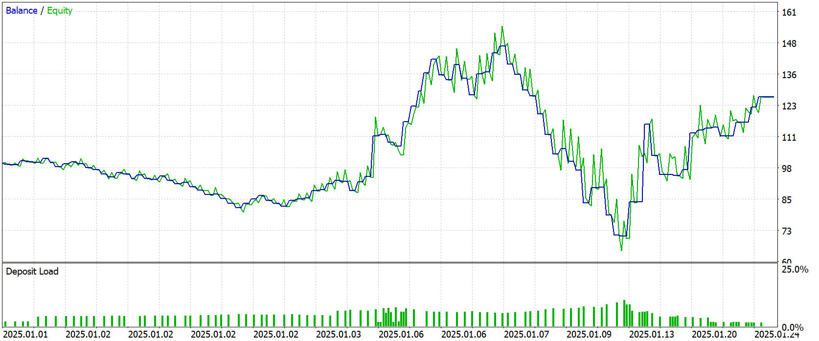
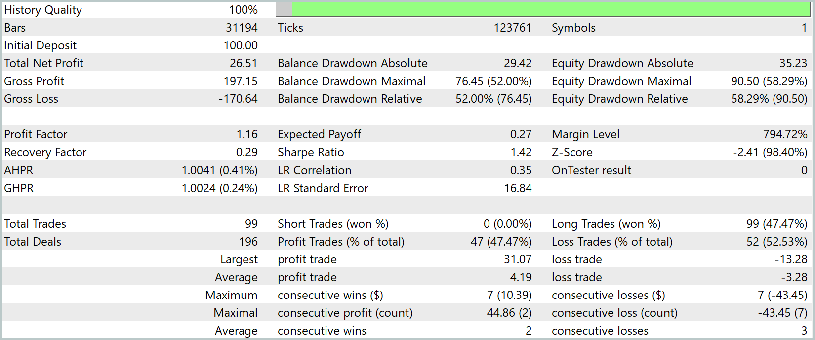
The test results can be described as encouraging, but with some caveats. The total return for the month was +26.5%, but the balance chart does not show a sustained upward trend. On the contrary, sideways movement is observed most of the time, with periods of instability and significant drawdowns. The maximum drawdown reached 58%, which indicates high volatility and unstable decisions in certain market situations.

This pattern suggests that the model is still in the process of finding a consistent trading style, rather than following a clear, profitable trajectory. Nevertheless, the positive outcome in itself is an encouraging sign: the foundation has been laid; now the task is to improve stability.

Conclusion

In the course of this work, we progressed from the concept of universal cross-domain time series forecasting to its practical implementation in the MetaTrader 5 environment. We examined the structure of the Encoder in detail, mastered the mechanism of multi-scale patching, and then integrated the resulting latent representations into the Actor–Director–Critic architecture. Every step — from data preparation and Self-Supervised training of the Encoder to offline and online fine-tuning of key modules — demonstrated how a well-balanced combination of cutting-edge research and engineering solutions can improve the quality of market dynamics analysis.

Testing on January 2025 market quotes showed that our system is capable of generating profits, although it is not without deep drawdowns. This underscores the importance of further refining risk management and adaptive loss-limitation mechanisms. At the same time, the very fact of positive returns without any additional parameter optimization indicates that the chosen architecture has a robust backbone and allows predictions to be made by reusing knowledge already gained.

References

• TimeFound: A Foundation Model for Time Series Forecasting
• Other articles in this series

Programs used in the article

#	Name	Type	Description
1	Research.mq5	Expert Advisor	Expert Advisor for collecting examples
2	ResearchRealORL.mq5	Expert Advisor	Expert Advisor for collecting examples using the Real-ORL method
3	StudyEncoder.mq5	Expert Advisor	Expert Advisor for training the environment encoder
4	Study.mq5	Expert Advisor	Expert Advisor for offline model training
5	StudyOnline.mq5	Expert Advisor	Online model training Expert Advisor
6	Test.mq5	Expert Advisor	Model testing Expert Advisor
7	Trajectory.mqh	Class Library	Structure for describing the system state and model architectures
8	NeuroNet.mqh	Class Library	A class library for building neural networks
9	NeuroNet.cl	Library	OpenCL program code library