Neural Networks in Trading: A Cross-Domain Time Series Forecasting Framework (TimeFound)

Introduction

Time series forecasting has long been an indispensable tool for financial analysts. If you've ever tried to predict where stock prices will go or how the volatility of a financial index will change, you know full well that it is like reading tea leaves. That said, no serious fund can survive without this kind of fortune-telling.

In the past, classical statistical models — such as ARIMA and exponential smoothing — were widely used. Come to think of it, even linear regression often proved useful. The arguments for why the model should be simpler sounded convincing — until deep neural networks entered the picture. Today, they do not merely bear fruit — they reap the harvest, impressing with their accuracy and speed in processing terabytes of historical data.

However, like any powerful weapon, deep models have their downsides. Training them requires a whole mine of labeled data for the specific task. Without this, the neural-network Big Brother simply won't work. But what should you do if you only have a limited amount of historical data, or if the market has just started trading? How can you predict the price of a newly issued token for which the broker's terminal has not yet accumulated any meaningful history? This is where the concept of Zero-Shot Forecasting comes in — an approach that allows the model to perform in settings where traditional methods are powerless.

Time-series researchers have drawn parallels with large language models (Large Language Models). LLMs are already highly successful with text: they translate, write poetry, and answer questions. Why not apply their ideas to forecasting price trends? That's how the boom in so-called Foundation Models for time series began. Imagine this: a single, universal model — and it does not matter whether it is predicting stock prices, electricity consumption, or the unemployment rate. The key is to train it properly using a diverse dataset.

Inspired by this idea of universality, the authors of the paper "TimeFound: A Foundation Model for Time Series Forecasting" introduced a new framework based on the Transformer architecture as a basis for time series forecasting: TimeFound. They took the best ideas from the world of NLP and adapted them for time series forecasting.

The TimeFound framework is built on the classic encoder-decoder architecture. The encoder analyzes a historical data series and extracts context from it. The decoder, in turn, projects the future while preserving causal relationships.

The model is based on a new approach to time series patching. Forget fixed window sizes. The framework's authors suggest splitting the sequence into several patches of different sizes at once. Imagine you are analyzing the behavior of a company’s stock: the monthly fluctuations look fairly uniform, while intraday movements are full of sharp jumps. Multi-resolution patching makes it possible to capture both scales: the long-term trend and volatility noise.

For pre-training, the framework's authors compiled a massive multi-domain dataset. All this diversity is necessary for the model to learn to identify universal patterns. The more data there is, the richer the vocabulary of patterns learned by the model becomes.

The training objective is simple: autoregressive forecasting. A set of historical data is fed into the model, and the model learns to predict subsequent values step by step. However, in this case, the forecast step may differ from the time step of the historical data. This is because the model returns results in the form of patches. A single patch may include multiple time steps of the system being analyzed.

The TimeFound Algorithm

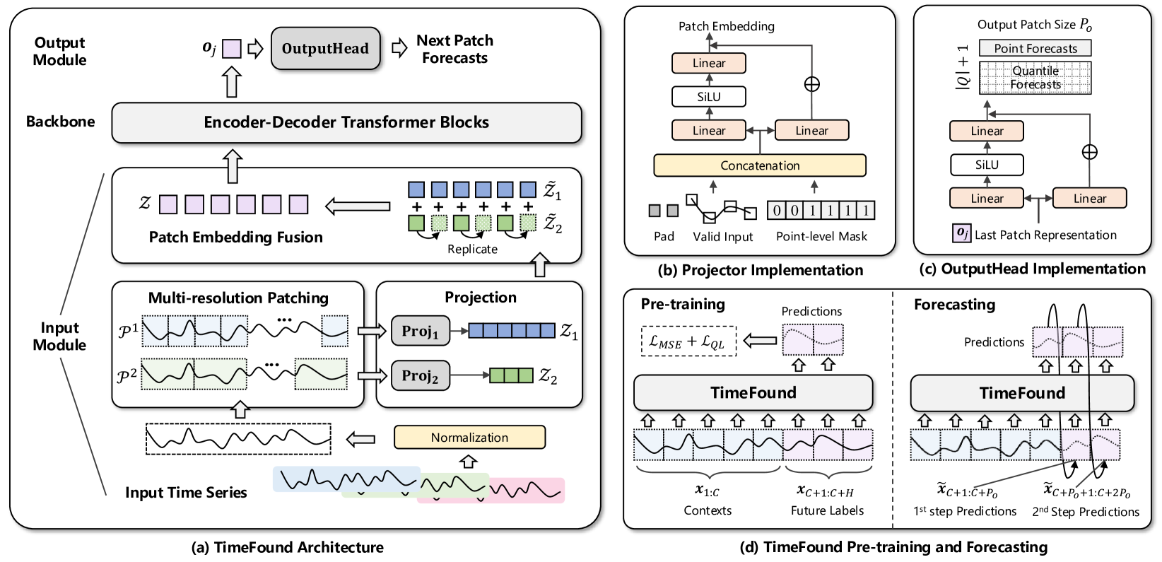
TimeFound is a universal model designed to serve as a foundation for building forecasting systems in various domains, including, but not limited to, financial markets. The model is built in an encoder–decoder format with a modular approach to data processing. It relies on normalization, multi-level patching, an attention mechanism with relative positioning, and joint training using point-forecast and quantile losses.

The framework's algorithm begins with thorough preparation of the input time series, because without a solid foundation, any forecast risks being unreliable. First, we bring the data into a comparable form — we normalize each series using standatization by subtracting the mean of the entire sequence from each data point and dividing by its standard deviation. Thanks to this technique, the model will not get confused when a market movement looks like a small sine wave compared to a massive increase in electricity consumption; conversely, it will detect even subtle fluctuations when they really matter.

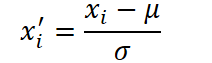
where μ and σ are the mean and standard deviation of the series X. This puts the data on the same scale without losing its temporal structure.

Once the scale has been adjusted, it is time to divide the time series into segments, or patches. In classical approaches, all patches are the same size, but we know that the same time series can contain both rapid spikes and slow trends. For this reason, the authors of the TimeFound framework propose multi-scale patching. At the first level, patches of the smallest scale are formed. This is where their number is greatest. As the level increases, the patch size also increases, while the number of patches decreases proportionally. In their work, the authors of the framework used patches whose sizes are powers of 2.

Each such patch captures a slice of the time series' dynamics, whether it is a brief spike in volatility or a prolonged downturn.

Next, a binary mask is added to the generated patches, indicating where the real data is and where there is only padding to a uniform size. Each such fragment of the time series then passes through its own two-layer perceptron with residual connections. These MLP projectors map patches of varying lengths into a unified d-dimensional latent space, where each vector reflects the essence of the local behavior of the series being analyzed.

However, not everything is ready yet. As mentioned earlier, during the multi-scale patching process, a different number of elements is generated at each level — there are several times more small blocks than large ones. To bring them together, the framework's authors suggest duplicating (replicating) the representations of large patches as many times as necessary to match their number to that of the smallest patches. As a result, we obtaina multi-channel representation aligned at each time step in which the vectors from all scales are merged. After that, their features are combined into a single latent matrix. It is this matrix that is fed into the attention block, enabling cross-scale interaction.

The model is based on an Encoder–Decoder with modified attention. The Encoder carefully examines the resulting sequence using bidirectional attention. This means that each position can ask all the other positions how events unfolded before and after it and, based on the weighted responses, form a deeper representation. At the same time, the attention mechanism relies on the relative positioning of patches: the model perceives a recent fragment (for example, three patches back) as more important than a distant one (say, twenty patches back), and assigns weights accordingly.

Once the Encoder has finished its work, its results are passed on to the Decoder, which can no longer access future target values and must rely solely on historical data. The attention mechanism does not allow the model to look further into the future than the aggregation of previously made predictions permits; therefore, each new prediction is accurate and caussally valid. Cross-Attention plays a key role here. As the Decoder constructs a representation of the next patch, it once again draws on the Encoder’s rich contextual vectors, extracting information about recent trends from them.

The Decoder's output is a predictive vector for the next patch — a concise description of preceding events and key signals. This vector is passed to the transformation module, which is implemented as a two-layer MLP with a residual connection. In this module, the latent representation is converted back into familiar time-series values, and a block of future points is generated at once. This batch generation of forecasts speeds up the model's operation and is particularly effective for long-term forecasting horizons.

When training the model, the framework's authors do not limit training to minimizing average prediction error. In addition to the standard MSE loss, which penalizes the squared difference between predicted and true values, they use a quantile loss function that forces the model to estimate uncertainty. For each time step, the model learns to output not only the mean values but also, say, the 10th, 50th, and 90th percentiles. A combined loss function that combines MSE and Quantile Loss strikes a balance between forecast accuracy and the width of the confidence interval.

Thus, the entire TimeFound algorithm is a unified, well-designed pipeline. It combines the power of transformers with the flexibility of multi-scale patching and sensitivity to uncertainty, enabling the model to handle any time series.

For pre-training TimeFound, the framework's authors compiled an extensive and heterogeneous dataset covering real and synthetic time series across various domains. Publicly available time series with different frequencies were collected, ranging from 5-minute to annual data. Data from financial markets (stock prices, currency futures), energy consumption, temperatures, and sales volumes were used. Their diversity was then increased through synthetic generation. This enables TimeFound to generate universal representations of time series, providing strong generalization without the need for fine-tuning on new tasks.

The authors’ visualization of the TimeFound framework is shown below.

Implementation in MQL5

After reviewing the theoretical aspects of the TimeFound framework, we move on to the practical part of our article, in which we use MQL5 to implement our own interpretation of the approaches proposed by the framework’s authors. But before diving into the details of the code, it is important to have a clear picture of the sequence of tasks and how they relate to one another. Our process begins with preparing the source data — and this is where the key to the quality of the entire subsequent forecast lies.

To normalize the data in the time series we're analyzing, we will not reinvent the wheel — we will use a ready-made batch normalization block. This module automatically scans the accumulated price buffer, calculates the mean and variance at each step, and normalizes the data distribution in real time, reducing sensitivity to abrupt distribution shifts caused by changing market conditions. Thanks to this sliding normalization, we preserve the dynamics of important patterns while removing the dispersion that interferes with stable training and prediction.

Once the data have been normalized to a single scale, it is time to tackle a truly critical task: multi-scale patching. In the classic sequential-replication approach, we would first split the series into fragments of different sizes, then pad them out to the same number of small blocks by simply copy-pasting large vectors, and only then slowly stitch everything back together. This method is straightforward, but unacceptable because of the latency. Every time a new candle arrives, we waste precious time on replication, and the resulting coarser-scale embeddings are duplicated several times, losing their uniqueness.

In our implementation, we will take a different approach. Let's use the concept of multi-window convolution. Imagine that, instead of three separate procedures, we run three convolutional layer kernels in parallel, each with its own window size. Thanks to zero padding and overlap, convolutional filters with the same stride slide neatly along the entire length of the time series being analyzed, simultaneously forming three feature arrays of the same length.

This approach provides us with several benefits at once. First, all computations run simultaneously — there is no need to wait for the small patches to be processed and then filled in with data from the larger ones. Second, because we use a sliding window with a fixed stride, each new value in the series is included in all three transformations, and we have no alignment issues. The output tensors are aligned to the same time index from the start. Third, thanks to the overlap, the larger filters' windows capture adjacent segments, making it easier to detect slow trends and smoothed fluctuations rather than just rigid blocks.

At the same time, we do not need to replicate or interpolate anything manually — the algorithm preserves the same number of elements and a uniform representation for each time step.

As a result, we get an instant, compact snapshot of the market picture at the required level of detail, ready for projection into the latent space of the MLP projector.

It is precisely this type of parallel, multi-scale patching that forms the core of the preprocessing module: it preserves the uniqueness of embeddings at every scale, eliminates redundant replication, and enables your trading robot to make decisions faster and more accurately, responding immediately to both micro-spikes and long-term trends.

Next, we move on to transforming the resulting embeddings into highly informative features. After multi-window convolution, the specified number of channels is already present at each time step in the form of embeddings. But that is not enough for a deep model. We need to add a layer of nonlinearity and trainable connections to obtain a truly expressive representation. In the original version, the authors of TimeFound propose a two-layer MLP with a pattern of residual connections. However, in our implementation, we use a prebuilt multi-head Feed-Forward block from the StockFormer framework.

Imagine that you have three streams of features at different scales, and each of them needs to be brought up to a common quality standard. Our module splits these streams into independent heads, each of which is processed in parallel with its own weights and biases. Then all the results are combined back into a single vector. Thanks to residual connections, information about the initial embeddings is preserved and smoothly combined with the layer output, which improves convergence and makes the model more robust to noise in the data.

Within this Feed-Forward block, each head is a two-layer MLP with a nonlinearity between the layers. The output of the MLP is added to the input data and normalized. Thus, the final vector at each time step represents a synthesis of local patterns and global features, ready to be passed to the next module.

This approach allows us to maintain conceptual alignment with the original TimeFound architecture while leveraging a proven and optimized component from StockFormer, which saves development time and ensures high real-time performance.

At the final stage of preparing the multi-scale features, we move on to aggregating them; here, a simple summation approach gives way to a more flexible mechanism: a sequence of convolution and max-pooling. Imagine that you have three embedding channels, and each one contributes to your understanding of what is happening. If these channels are added element-wise, they will all be assigned the same weight, regardless of how significant short-term spikes or long-term trends are over this interval. Instead, we run a convolution in which trainable filters analyze values across different scales and identify the most informative combinations.

As the convolutional layer passes over the three-channel tensor, each filter sees all scales at once and searches for characteristic patterns within them. The result is a set of new features, each of which reflects a combination of local and global signals. And this is where max-pooling comes into play: as it slides over the resulting feature maps, it retains only the strongest responses, ignoring noise and insignificant fluctuations. Thus, if, within the same time interval, the micro-level records a sharp spike in volume while the macro-level shows steady growth, pooling ensures that both signals are adequately represented in the final vector.

As a result of this combination of convolution and max-pooling, we no longer need to manually set weights for each scale. The model learns on its own to focus on the set of features that is most relevant to the current prediction. This adaptive mechanism not only improves inference accuracy but also makes the algorithm more resilient to market jumps and noise, since weak or infrequent signals are smoothed out, whereas important spikes are amplified and reach the Encoder and Decoder stages without loss.

We implement the approach described above within the CNeuronTimeFoundPatching object, whose structure is shown below.

class CNeuronTimeFoundPatching   :  public CNeuronConvOCL
  {
protected:
   CNeuronTransposeOCL              cToVarSeq;
   CNeuronMultiWindowsConvWPadOCL   cProjecting;
   CNeuronTransposeVRCOCL           cToVarProjSeq;
   CNeuronMultiWindowsConvWPadOCL   cPatchingProj;
   CNeuronMHFeedForward             cPatchsFeedForward;
   CNeuronConvOCL                   cPatchingAgr;
   CNeuronProofOCL                  cProof;
   CNeuronTransposeOCL              cToPatchVarEmb;
   //---
   virtual bool      feedForward(CNeuronBaseOCL *NeuronOCL) override;
   virtual bool      updateInputWeights(CNeuronBaseOCL *NeuronOCL)  override;
   virtual bool      calcInputGradients(CNeuronBaseOCL *NeuronOCL)  override;

public:
                     CNeuronTimeFoundPatching(void) {};
                    ~CNeuronTimeFoundPatching(void) {};
   //---
   virtual bool      Init(uint numOutputs, uint myIndex, COpenCLMy *open_cl,
                          uint count, uint patchs, uint variables,
                          uint embedding_size, uint patch_filters,
                          ENUM_OPTIMIZATION optimization_type, uint batch);
   //---
   virtual bool      Save(int const file_handle) override;
   virtual bool      Load(int const file_handle) override;
   //---
   virtual int       Type(void)  override const {  return defNeuronTimeFoundPatching; }
   //---
   virtual void      SetOpenCL(COpenCLMy *obj) override;
   virtual bool      WeightsUpdate(CNeuronBaseOCL *source, float tau) override;
  };

All internal CNeuronTimeFoundPatching modules operate independently from the moment the program starts. They are declared statically and are initialized when the library is loaded. Therefore, we do not need to create them in the constructor or worry about cleanup in the destructor: these methods remain empty, and all the magic of managing the object's architecture is handled by a single universal Init method.

In the initialization method's parameters, we receive a set of constants that define the architecture of the internal objects.

bool CNeuronTimeFoundPatching::Init(uint numOutputs, uint myIndex, COpenCLMy *open_cl,
                                    uint count, uint patchs, uint variables,
                                    uint embedding_size, uint patch_filters,
                                    ENUM_OPTIMIZATION optimization_type, uint batch)
  {
   uint inside_emb = MathMax((embedding_size + 2) / 6, 8);
   if(!CNeuronConvOCL::Init(numOutputs, myIndex, open_cl, 3 * inside_emb, 3 * inside_emb,
                            embedding_size, patchs * variables, 1, optimization_type, batch))
      return false;
   SetActivationFunction(SoftPlus);

It should be noted that when building this object, we borrowed the best ideas from the Mantis framework. Instead of hard-coded patch sizes, our class accepts only the number of segments for the finest level and the desired output token size as input. This provides flexibility — you can quickly change the granularity of patching without editing the code.

But we took it a step further. Mantis used a single convolution to generate feature channels, while we implemented multi-window convolution, which creates several levels of representation of the input signal at once. When the initialization phase begins, our task is to calculate the internal size of the token vector for each level of detail. The user can specify any token length for the object's output. However, it will not always be divisible by the number of levels without a remainder. This is where the parent convolutional class comes into play: it carefully adjusts the number of channels to the specified size, applying its optimized filters and ensuring a consistent, uniform representation of the features.

As before, we expect the object to take as input a two-dimensional tensor describing a multimodal time series, where each row represents a detailed description of a single time step. However, in order for our patching pipeline to treat individual features as individual univariate sequences, we first transpose the input data matrix.

This simple but important technique ensures that all subsequent operations will follow the strict principle of “one series, one story”, rather than mixing signals from different sources. This is exactly how we preserve the integrity and interpretability of each time series.

int index = 0;
  if(!cToVarSeq.Init(0, index, OpenCL, count, variables, optimization, iBatch))
     return false;  

Next up is the multi-window convolution. We run three filters simultaneously with window sizes of 3, 7, and 8 bars and a stride of 1. Thanks to zero padding, the length of the output sequences remains the same, but each value is now enriched with knowledge of its nearest neighbors and their context.

index++;
  {
   int windows[] = {3, 5, 7};
   if(!cProjecting.Init(0, index, OpenCL, windows, 1, inside_emb, count, variables,
                        optimization, iBatch))
      return false;
   cProjecting.SetActivationFunction(SoftPlus);
  }

At this stage, we have successfully generated the basic features for further analysis. Now we need to structure this data so it can be fed into the subsequent blocks of the model — in other words, perform patching. But before dividing the time series into segments, it is necessary to perform an important technical operation: reorder the last axes in the resulting four-dimensional tensor.

The tensor generated in the previous step has the shape [Variable × Series Length × Number of Channels × Number of Features], where each time step is represented by a three-channel vector obtained at different convolution scales. However, to make it easier to work with individual univariate sequences that will be segmented independently, we need to format the data as `[Variable × Number of Channels × Number of Features × Series Length]`. This allows each feature to be processed as a separate time series and subsequently split into fixed-length segments — patches.

index++;
if(!cToVarProjSeq.Init(0, index, OpenCL, variables, count, 3 * inside_emb, optimization, iBatch))
   return false;

This representation is particularly useful in a financial context: each channel, enriched by multi-window convolution, now acts as an independent market indicator whose dynamics can be analyzed through patching.

Next, we move on to a key stage — multi-scale patching — which forms the foundation of our time series preprocessing architecture. Here, we are implementing a concept inspired not so much by traditional approaches as by the actual practice of high-frequency market data analysis, where both the depth of coverage and the speed of response are crucial.

Instead of dividing the sequence into patches in a rigid, one-dimensional way, we use a multi-window convolution layer, which allows us to work across multiple scales simultaneously. This allows the model to view the market across different time horizons—much like an analyst who looks simultaneously at 1-minute candles, hourly charts, and the daily chart.

index++;
  {
   uint step = (count + patchs) / (patchs + 1);
   uint windows[] = {step, 3 * step / 2, 2 * step};
   if(!cPatchingProj.Init(0, index, OpenCL, windows, step, patch_filters, patchs,
                          3 * inside_emb * variables, optimization, iBatch))
      return false;
   cPatchingProj.SetActivationFunction(SoftPlus);
  }

In this case, the convolution window sizes are determined automatically — they depend on the length of the time series being analyzed and on the number of patches specified by the user. At higher scales, this value is scaled upward with overlap to ensure the coherence and continuity of information between patches.

In the next step, the pre-extracted patches are fed into the multi-head FeedForward module. This is not just a formality — this is where the real work of making sense of the data begins. Each patch obtained at different scales is now converted into a full-fledged embedding — that is, a compact, information-rich representation that encodes the key characteristics of the corresponding time series segment. The module produces a set of compact yet expressive vectors, each of which can be considered the quintessence of the corresponding time segment.

index++;
if(!cPatchsFeedForward.Init(0, index, OpenCL, 3 * patch_filters, 6 * patch_filters, patchs,
                            3 * inside_emb * variables, 3, optimization, iBatch))
   return false;
index++;

Once we have obtained expressive embeddings for each patch at all scales, we move on to the data aggregation stage. After all, for a model to form a comprehensive picture of the current market context, it must combine information from different levels of detail into a single feature vector.

To solve this problem, we use a combination of convolution and max-pooling. The convolution layer allows us to identify local dependencies between embeddings at different scales. It acts as an analyst who looks for characteristic combinations of short- and long-term patterns — for example, short-term volatility against the backdrop of a steady long-term trend. Such combinations often prove to be crucial when making trading decisions, especially in complex market conditions.

Next, the data undergo max-pooling, which extracts the strongest, most distinctive features in each region of the resulting tensor. As a result, we obtain a single aggregated feature vector. This is a compact yet informative representation of the entire input history, processed at multiple scales.

index++;
if(!cPatchingAgr.Init(0, index, OpenCL, 3 * patch_filters, 3 * patch_filters, patch_filters,
                      patchs, 3 * inside_emb * variables, optimization, iBatch))
   return false;
cPatchingAgr.SetActivationFunction(SoftPlus);
index++;
if(!cProof.Init(0, index, OpenCL, patch_filters, patch_filters, 3 * patchs * inside_emb * variables,
                optimization, iBatch))
   return false;

But before passing the resulting tokens further along the architecture, we need to perform one more important step: transpose the resulting tensor, bringing the time axis back to the front.

   index++;
   if(!cToPatchVarEmb.Init(0, index, OpenCL, variables * 3 * inside_emb, patchs, optimization, iBatch))
      return false;
//---
   return true;
  }

Why is this necessary? The reason is that in the previous stages — specifically, when forming embeddings and aggregating patches — the data were represented in a format that focused primarily on patches and features. This axis order is convenient for local processing, but it is not suitable for mechanisms that are sensitive to temporal order.

By returning the time axis to the beginning, we effectively arrange the resulting tokens in chronological order. Each token now corresponds to a time step enriched with information from multiple scales. This allows the model to interpret the data as a full-fledged temporal sequence rather than as an abstract set of features.

It is in this form that the tensor is passed on to the next stages of processing — where temporal dependencies, context analysis, and forecast generation come into play. This ordering preserves the causal-temporal relationship in the data; without it, any attempt to model a financial market would be meaningless.

Despite the apparent complexity of the object's internal architecture, the implementation of the algorithms for the forward and backward passes remains extremely straightforward. The computational logic is organized step by step and sequentially, without nested loops or convoluted branching. I think it will not be hard to understand how these methods work. For this reason, we have deliberately chosen not to discuss them in detail in this article. For anyone interested in delving deeper into the technical implementation of the CNeuronTimeFoundPatching object, the complete source code — including all of its methods — will be available as an attachment to this article.

We have gradually reached the reasonable limits imposed by the article format. The volume of material is already quite substantial. However, as you can see, our work is still far from complete. We have only laid the groundwork and implemented a critically important data preprocessing module, which forms the basis for all subsequent analysis.

Let's take a short break, catch our breath, and then continue in the next article, implementing the remaining components of the framework we have discussed, step by step.

Conclusion

In this article, we explored the theoretical aspects of TimeFound — a framework capable of transforming the chaotic structure of time series data into a formalized, predictable pattern.

We have begun implementing our own interpretation of the approaches proposed by the framework's authors. We focused primarily on the data preprocessing module, since it is this module that determines how accurately and expressively the model can capture the structure of the input signal.

Equally interesting work lies ahead, and we will dive into it in the next article.

References

• TimeFound: A Foundation Model for Time Series Forecasting
• Other articles in the series

Programs used in the article

#	Name	Type	Description
1	Research.mq5	Expert Advisor	Expert Advisor for collecting samples
2	ResearchRealORL.mq5	Expert Advisor	Expert Advisor for collecting examples using the Real-ORL method
3	StudyEncoder.mq5	Expert Advisor	Expert Advisor for training the environment encoder
4	Study.mq5	Expert Advisor	Expert Advisor for offline model training
5	StudyOnline.mq5	Expert Advisor	Expert Advisor for online model training
6	Test.mq5	Expert Advisor	Expert Advisor for testing the model
7	Trajectory.mqh	Class Library	Structure describing the system state and model architecture
8	NeuroNet.mqh	Class Library	Class library for creating a neural network
9	NeuroNet.cl	Library	Code library for an OpenCL program