Neural Networks in Trading: Heterogeneity-Informed Meta-Parameter Learning (Conclusion)

Introduction

Algorithmic trading rarely forgives excessive complexity or unjustifiably simplistic solutions. Any model — whether it is a highly complex neural network ensemble or a minimalist autoregressive filter — must ultimately stand the test of time and the market. It was precisely from this perspective that HimNet was conceived — a framework that does not seek to impress with the number of trainable parameters or the exotic nature of its computations. On the contrary, it focuses on delivering stable, reproducible, and economically meaningful results.

From the very beginning, HimNet demonstrates three qualities that set it apart from many other approaches. First, there is the rationality of the architecture: it contains no overloaded layers that merely create the illusion of depth of analysis. Every module here is functional and justified. Second, there is measured adaptability: instead of mindlessly adjusting to the noise of every market fluctuation, the framework strikes a balance between flexibility and stability. And third, minimalism in parameter management. HimNet is designed so that the number of trainable coefficients is reduced to the necessary minimum. This helps avoid excessive fitting to historical data and preserve predictive power even on distant segments of time series.

In our previous works, we systematically explored the internal mechanics of this framework. Starting with the theoretical foundations, we examined in detail the methods for generating embeddings and analyzed how recurrent and convolutional components complement each other. The HimNet architecture is like a well-coordinated mechanism, where every cog — whether it is a Chebyshev polynomial block or the GCRU mechanism — has its own precise role. This is not a pile-up of technologies, but a carefully calculated design that enables an informative representation of the market without any loss of processing speed or excessive complication of the computational chain.

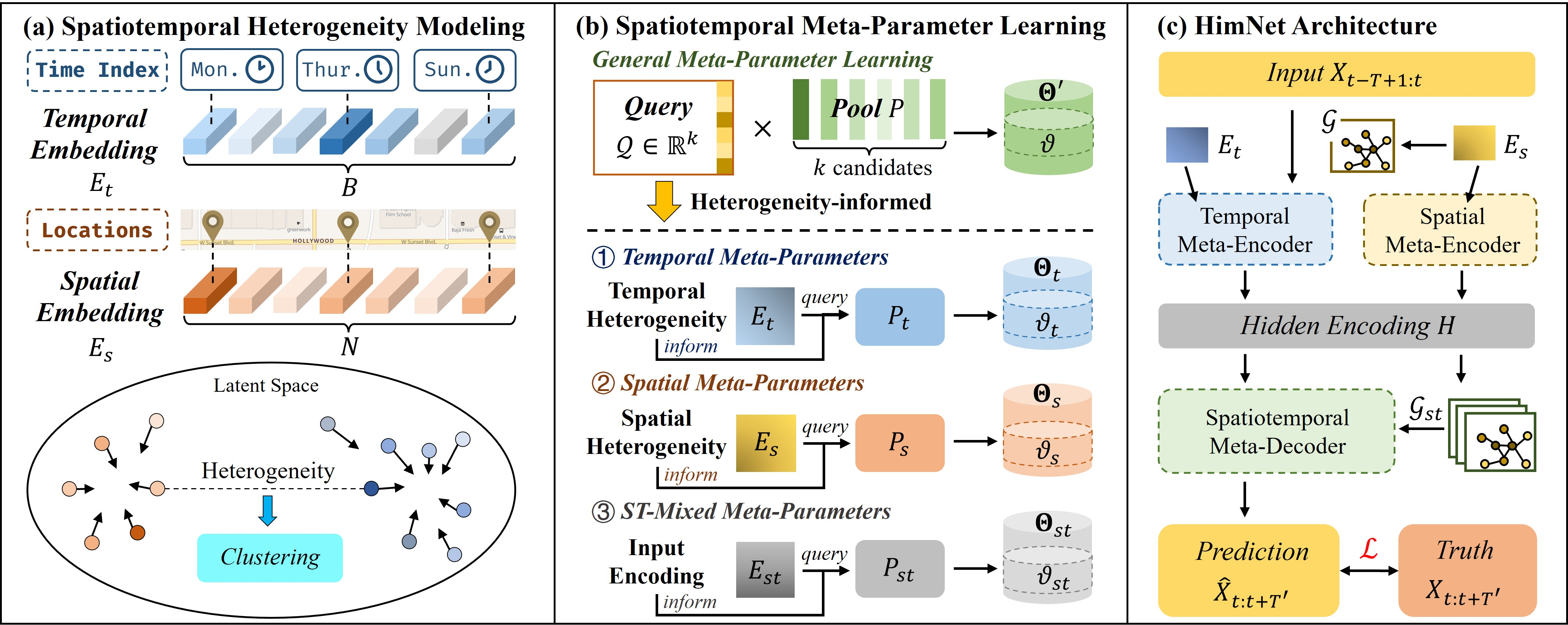
The HimNet framework is built on the classic and, in many ways, time-tested Encoder–Decoder architecture. This scheme has proven effective in tasks involving the processing of complex sequences, where it is important not only to capture the current state of the market, but also to extract stable patterns from it for further forecasting. The Encoder and Decoder are based on the same foundation: they both use trainable embeddings and graph recurrent blocks (GCRU). However, there is a subtle but important difference between them — in the very way embeddings are formed.

In the Encoder, temporal and spatial embeddings are extracted directly from predefined sets, and they are used as a kind of query to pools of meta-parameters. This allows the Encoder to adapt to the context.

The Decoder, on the other hand, generates embeddings indirectly — based on a latent representation synthesized from the outputs of the Encoder. It projects the hidden representation into a spatiotemporal embedding, which becomes a query to the ST meta-parameter model, allowing the Decoder to generate weights.

We have already done a great deal of preparatory work: we have implemented the fundamental components of the model, including graph recurrent blocks capable of effectively accounting for spatiotemporal dependencies in the data. Now it is time to move up to the next level of the hierarchy — building a full-fledged structure for the Encoder and Decoder. This stage will serve as a bridge between the individual elements of the framework and its practical application. It is here that abstract blocks become interconnected, and the data flow begins to form a meaningful representation of future market states.

Encoder

The authors of the HimNet framework provided a two-stream data processing mechanism, in which a separate Encoder is responsible for each type of dependency: spatial and temporal. This approach makes it possible to avoid mixing different signal structures together and instead examine them in parallel branches, ensuring a more accurate and clean identification of key patterns. Following the ideas presented, today we will begin by building a Temporal Encoder. After all, time is the very thread upon which all market dynamics are woven.

Temporal Encoder

The CNeuronHimNetTempEncoder object is a kind of temporal filter within the framework, designed to extract patterns hidden in sequences of quotes and market patterns. What is more, it does this on several scales at once.

class CNeuronHimNetTempEncoder   : public CNeuronBaseOCL
  {
protected:
   uint              aTimeframes[2];
   CCircleParams     caEmbeddings[2];
   CNeuronBaseOCL    cConcatEmbeddings;
   CLayer            cGRCUs;
   CBufferFloat      bSupportAccum;

public:
                     CNeuronHimNetTempEncoder(void) {};
                    ~CNeuronHimNetTempEncoder(void) {};
   //---
   virtual bool      Init(uint numOutputs, uint myIndex, COpenCLMy *open_cl,
                          uint units, uint window, uint window_out, uint cheb_k,
                          uint layers, uint embed_dim, uint period1,
                          uint timeframe1, uint period2, uint timeframe2,
                          ENUM_OPTIMIZATION optimization_type, uint batch);
   //---
   virtual bool      feedForward(CNeuronBaseOCL *NeuronOCL,
                                 CChebPolinom *Support,
                                 int label);
   virtual bool      calcInputGradients(CNeuronBaseOCL *NeuronOCL,
                                        CChebPolinom *Support);
   virtual bool      updateInputWeights(CNeuronBaseOCL *NeuronOCL,
                                        CChebPolinom *Support);
   //---
   virtual int       Type(void)   const   {  return defNeuronHimNetTempEncoder;   }
   //--- methods for working with files
   virtual bool      Save(int const file_handle) override;
   virtual bool      Load(int const file_handle) override;
   //---
   virtual bool      WeightsUpdate(CNeuronBaseOCL *source, float tau) override;
   virtual void      SetOpenCL(COpenCLMy *obj) override;
   virtual void      SetActivationFunction(ENUM_ACTIVATION value) override { };
   virtual bool      Clear(void) override;
   //---
   virtual uint      GetCount(void) const;
   virtual uint      GetWindowIn(void) const;
   virtual uint      GetWindowOut(void) const;
   virtual uint      GetChebK(void) const;
//---
   virtual bool      SetGradient(CBufferFloat *buffer, bool delete_prev = true);
  };

The key elements are two embedding sets represented by the caEmbeddings array. Each of these dictionaries stores not complete data, but only compact representations of individual time steps — embeddings that serve as queries to the model’s parameter pools. This means that each time step effectively accesses its own parameter subspace, retrieving the required value and thereby configuring the subsequent data flow.

It is important to emphasize that both embedding sets operate in a coordinated yet independent manner — this allows the model to look at two time scales simultaneously and avoid confusing short-term noise with long-term inertia. We'll examine in detail how these queries interact with the data stream and what tasks the other components of the Temporal Encoder handle as we implement the methods.

All internal objects are declared statically, so the constructor and destructor remain minimal. The actual initialization of the entire set of declared components and inherited objects is performed centrally in the Init method.

bool CNeuronHimNetTempEncoder::Init(uint numOutputs, uint myIndex, COpenCLMy *open_cl,
                                    uint units, uint window, uint window_out, uint cheb_k,
                                    uint layers, uint embed_dim, uint period1,
                                    uint timeframe1, uint period2, uint timeframe2,
                                    ENUM_OPTIMIZATION optimization_type, uint batch)
  {
   if(layers <= 0)
      return false;

The algorithm begins with a small control block — we check the number of internal layers in the Encoder. If the value of the layers parameter is less than or equal to 0, the method fails immediately. This prevents pointless configurations: if there are no layers, there is nothing to learn.

Next, the method of the same name in the parent class is called, and the object's basic parameters are passed to it. At this step, we define the shape of the tensor for the Encoder's output and reserve the necessary resources. If the basic initialization fails, there is no point in continuing the operations — the method returns false.

   if(!CNeuronBaseOCL::Init(numOutputs, myIndex, open_cl, window_out * units, optimization_type, batch))
      return false;

Next, the embedding sets are prepared, and the time step size is immediately stored in the corresponding elements of the aTimeframes array.

   int index = 0;
   if(!caEmbeddings[0].Init(0, index, OpenCL, embed_dim, period1, optimization, iBatch))
      return false;
   aTimeframes[0] = MathMax(1, timeframe1);
   index ++;
   if(!caEmbeddings[1].Init(0, index, OpenCL, embed_dim, period2, optimization, iBatch))
      return false;
   aTimeframes[1] = MathMax(1, timeframe2);
   if(!cConcatEmbeddings.Init(numOutputs, myIndex, open_cl, 2 * embed_dim, optimization_type, batch))
      return false;

Each embedding dictionary is configured for its own temporal granularity: the embedding size and period determine exactly which temporal queries will be sent to the parameter pool. If any of these initializations fail, the method aborts — we do not allow a partially assembled Encoder.

After the dictionaries are defined, cConcatEmbeddings is created — an object that will combine the two embeddings into a single vector.

Next, construction of the GRCU layers begins. First, we clear the cGRCUs container and explicitly bind the OpenCL context.

   cGRCUs.Clear();
   cGRCUs.SetOpenCL(OpenCL);
   index++;
   CNeuronHimNetGCRU *temp = new CNeuronHimNetGCRU();
   if(!temp ||
      !temp.Init(0, index, OpenCL, units, window, window_out, cheb_k, 2 * embed_dim, optimization, iBatch) ||
      !cGRCUs.Add(temp))
      return false;

Next, the first CNeuronHimNetGCRU object is created and initialized with the parameters of the first layer: for this layer, the number of input features is set equal to the corresponding dimension of the time series being analyzed, and the output dimension is set to that of the latent representation. This first layer is the bottom of the stack.

If initialization is successful, the layer is added to the cGRCUs container. If the addition or initialization fails, we return false.

For all subsequent layers, the logic becomes slightly simpler. Additional CNeuronHimNetGCRU objects are created in the loop, but now the input and output tensors have the same dimensions. This is a standard technique: the first layer expands and gathers the context, while the subsequent layers further refine this context in depth. In the event of any failure — whether during creation, initialization, or addition — we gracefully exit by returning false from the method to ensure the system is not left in an inconsistent state.

   for(uint i = 1; i < layers; i++)
     {
      index++;
      temp = new CNeuronHimNetGCRU();
      if(!temp ||
         !temp.Init(0, index, OpenCL, units, window_out, window_out, cheb_k, 2 * embed_dim, optimization, iBatch) ||
         !cGRCUs.Add(temp))
         return false;
     }

Once the GRCU stack has been formed, we initialize the auxiliary buffer bSupportAccum, which will be used to accumulate the error gradients of the Chebyshev polynomials obtained from the various layers of the Encoder.

   bSupportAccum.BufferFree();
   bSupportAccum.Clear();
   if(!bSupportAccum.BufferInit(units * units * cheb_k, 0) ||
      !bSupportAccum.BufferCreate(OpenCL))
      return false;

Next comes an important practical step: the output of the Encoder is the output of the last object in the cGRCUs container. To avoid unnecessary copying of large tensors, we synchronize the activation functions as well as the pointers to the result and gradient buffers. In other words, the Encoder adopts the activation semantics of the last layer and directs its external interfaces directly to the internal buffers of the last GRCU. This results in significant savings in memory and time.

   SetActivationFunction((ENUM_ACTIVATION)temp.Activation());
   if(!SetOutput(temp.getOutput(), true) ||
      !SetGradient(temp.getGradient(), true))
      return false;
//---
   return true;
  } 

After initializing the object, we move on to the core functionality of the Temporal Encoder: creating the forward pass method feedForward.

bool CNeuronHimNetTempEncoder::feedForward(CNeuronBaseOCL *NeuronOCL, CChebPolinom *Support, int label)
  {
   for(uint i = 0; i < caEmbeddings.Size(); i++)
     {
      int position = (label / int(aTimeframes[i])) % caEmbeddings[i].GetPeriod();
      if(!caEmbeddings[i].SetPosition(position) ||
         !caEmbeddings[i].FeedForward())
         return false;
     }
   if(!Concat(caEmbeddings[0].getOutput(), caEmbeddings[1].getOutput(),
              cConcatEmbeddings.getOutput(), 1, 1, caEmbeddings[0].Neurons()))
      return false;

Its algorithm begins by retrieving embeddings from our dictionaries. The operation is organized as a loop that sequentially iterates through the dictionaries in the array. For each dictionary, we calculate the current position based on the timestamp received from an external program. Then we generate a specific temporal embedding by calling the FeedForward method of the corresponding dictionary.

Essentially, this is the place where time is converted into an address for obtaining specialized weights. To use a trading analogy: when a specific time window occurs, we select the appropriate model configuration without retraining it — we simply use a different query.

Once both embeddings have been obtained, their results are combined into a single tensor.

Then comes the key part: passing through the GRCU container. The local variable inputs is initialized with a pointer to the source data object. In the loop over the elements of the cGRCUs container, we sequentially take each layer and call its forward pass method.

   CNeuronBaseOCL *inputs = NeuronOCL;
   CNeuronHimNetGCRU *current = NULL;
   for(int i = 0; i < cGRCUs.Total(); i++)
     {
      current = cGRCUs[i];
      if(!current ||
         !current. Feedforward(inputs, Support, cConcatEmbeddings.AsObject()))
         return false;
      inputs = current;
     }
//---
   return true;
  }

It is important to understand the contract: the first GRCU receives the raw data of the sequence being analyzed and a shared embedding query. It forms its own hidden representation. After that, the pointer in inputs is replaced with the current object — the output of the first layer becomes the input for the next one. This is how a stack of sequential transformations is built: the first layer expands the context, while the subsequent layers refine and compress the representation. In trading practice, this is similar to an initial analytical pass, where all the details are gathered, while the subsequent layers — like more experienced managers — filter, aggregate, and prepare the signal for output.

The Chebyshev polynomial buffer (Support) serves as the core of graph aggregation (K-hop). Passing the same object to each layer ensures a consistent view of the structure of relationships between individual sequences throughout the entire stack, while each GRCU uses its own meta-parameters (generated from the embedding) to interpret this Support.

Now that we have gone over the forward pass, it makes sense to move on to the backward pass — to the point where the model is evaluated, and we carefully assign responsibility for the error to all of its components. The calcInputGradients method is precisely the procedure in which the errors accumulated at the Encoder output are propagated back through the GRCU stack and the embedding sets, adjusting the behavior of each component.

bool CNeuronHimNetTempEncoder::calcInputGradients(CNeuronBaseOCL *NeuronOCL, CChebPolinom *Support)
  {
   if(!NeuronOCL || !Support)
      return false;

First, the method uses a protected check to make sure that it has been given valid pointers as input. Next, the input source for the last layer is determined. If there is more than one layer in the stack, we take the penultimate GRCU; otherwise, we take the source data object. We start distributing the error gradients with the last GRCU — the very object whose result we designated as the Encoder's external output during initialization. This makes sense: the gradient first reaches the top of the stack and then begins to propagate downward from there.

   CNeuronBaseOCL *inputs = (cGRCUs.Total() > 1 ? cGRCUs[-2] : NeuronOCL);
   CNeuronHimNetGCRU* current = cGRCUs[-1];
   if(!current ||
      !current.calcInputGradients(inputs, Support, cConcatEmbeddings.AsObject()))
      return false;
   if(!DeConcat(caEmbeddings[0].getGradient(), caEmbeddings[1].getGradient(),
                cConcatEmbeddings.getGradient(), 1, 1, caEmbeddings[0].Neurons()))
      return false;

This is where the main local work takes place: the last GRCU distributes the received gradient among its input, internal meta-parameters, and the Chebyshev polynomial gradient buffer (Support). It is important to understand that, at this point, Support serves as a shared connection map, and each layer in the stack can contribute to it. That is why we need an accumulation mechanism.

The next step is to split the gradient of the combined embedding back into two parts — the gradients of the two embedding sets. We return each branch's own contribution to the error so that the dictionaries can later adjust their queries to the parameter pools.

If there is more than one layer in the stack, a careful process of accumulating gradients for Support begins. First, we store a pointer to the current gradient buffer in the local variable temp so that we do not lose the previous buffer with the values accumulated earlier. Next, we temporarily redirect the error gradients to the preallocated bSupportAccum buffer.

   if(cGRCUs.Total() > 1)
     {
      CBufferFloat *temp = Support.getGradient();
      if(!Support.SetGradient(GetPointer(bSupportAccum), false))
         return false;
      for(int i = cGRCUs.Total() - 2; i >= 0; i--)
        {
         current = cGRCUs[i];
         inputs = (i > 0 ? cGRCUs[i - 1] : NeuronOCL);
         if(!current ||
            !current.calcInputGradients(inputs, Support, cConcatEmbeddings.AsObject()))
            return false;
         if(!SumAndNormilize(temp, Support.getGradient(), temp, 1, false, 0, 0, 0, 1))
            return false;
         if(!DeConcat(caEmbeddings[0].getPrevOutput(), caEmbeddings[1].getPrevOutput(),
                      cConcatEmbeddings.getGradient(), 1, 1, caEmbeddings[0].Neurons()))
            return false;
         for(uint i = 0; i < caEmbeddings.Size(); i++)
            if(!SumAndNormilize(caEmbeddings[i].getGradient(), caEmbeddings[i].getPrevOutput(),
                                caEmbeddings[i].getGradient(), 1, false, 0, 0, 0, 1))
               return false;
        }
      if(!Support.SetGradient(temp, false))
         return false;
     }
//---
   return true;
  }

In a loop that iterates through the stack objects in reverse order, we call the error gradient propagation method for each layer. Next, we aggregate the new contribution with the one already accumulated in the temp buffer. After that, we again split the gradient of the combined embedding into two information streams. Finally, for each dictionary, we add the values we've obtained to the ones we've accumulated so far.

After iterating through all the layers, we reset the pointers to the data buffers to their initial state. This is important: only in this way will external optimizers see the correct signal for updating the parameters underlying graph aggregation.

After successfully completing all iterations, the method returns true, which indicates that the gradient has been successfully propagated through all components of the Encoder down to the source data level.

After the gradients have been carefully collected, the next step is to update the parameters. The updateInputWeights method is simple in form but important in substance: it sequentially passes control to the internal components that contain trainable weights. It does this in the same order in which the computational sequence is implemented.

bool CNeuronHimNetTempEncoder::updateInputWeights(CNeuronBaseOCL *NeuronOCL, CChebPolinom *Support)
  {
   for(uint i = 0; i < caEmbeddings.Size(); i++)
      if(!caEmbeddings[i].UpdateInputWeights())
         return false;

First, both embedding sets are updated in the loop. Each call to UpdateInputWeights applies the gradients accumulated in the previous step to the parameters of the corresponding dictionary.

The method then traverses the GRCU stack in forward order: each layer is responsible for locally updating the parameters of its embeddings and meta-pools.

   CNeuronBaseOCL* inputs = NeuronOCL;
   CNeuronHimNetGCRU* current = NULL;
   for(int i = 0; i < cGRCUs.Total(); i++)
     {
      current = cGRCUs[i];
      if(!current.updateInputWeights(inputs, Support, cConcatEmbeddings.AsObject()))
         return false;
      inputs = current;
     }
//---
   return true;
  }

The complete source code for this class, including the implementation of all methods, is attached; it contains all the details discussed above. With that, our analysis of the Temporal Encoder can be considered complete, and we are ready to move on.

Spatial Encoder

Before we move on, let's discuss what the spatial Encoder is and how it differs from the Temporal Encoder; after all, understanding this difference is important for proper integration into the overall HimNet architecture.

The Temporal Encoder operated on a set of embedding sets that served as queries to parameter pools for different temporal granularities. The Spatial Encoder, by contrast, does not require a large number of periodic keys — the structure of the spatial data in this problem is stable. Therefore, instead of dictionaries, we use a single set of trainable parameters encapsulated in the cEmbedding object. This allows the model to have a single centralized representation of the market space, which is refined during training and then used as a continuous source of contextual queries for GRCU.

class CNeuronHimNetSpatEncoder   :     public CNeuronBaseOCL
  {
protected:
   CParams           cEmbedding;
   CLayer            cGRCUs;
   CBufferFloat      bSupportAccum;
   CBufferFloat      bEmbeddingAccum;

public:
                     CNeuronHimNetSpatEncoder(void) {};
                    ~CNeuronHimNetSpatEncoder(void) {};
   //---
   virtual bool      Init(uint numOutputs, uint myIndex, COpenCLMy *open_cl,
                          uint units, uint window, uint window_out, uint cheb_k,
                          uint layers, uint embed_dim,
                          ENUM_OPTIMIZATION optimization_type, uint batch);
   //---
   virtual bool      feedForward(CNeuronBaseOCL *NeuronOCL,
                                 CChebPolinom *Support);
   virtual bool      calcInputGradients(CNeuronBaseOCL *NeuronOCL,
                                        CChebPolinom *Support);
   virtual bool      updateInputWeights(CNeuronBaseOCL *NeuronOCL,
                                        CChebPolinom *Support);
   //---
   virtual int       Type(void)   const   {  return defNeuronHimNetSpatEncoder;   }
   //--- methods for working with files
   virtual bool      Save(int const file_handle) override;
   virtual bool      Load(int const file_handle) override;
   //---
   virtual bool      WeightsUpdate(CNeuronBaseOCL *source, float tau) override;
   virtual void      SetOpenCL(COpenCLMy *obj) override;
   virtual void      SetActivationFunction(ENUM_ACTIVATION value) override { };
   virtual bool      Clear(void) override;
   //---
   virtual uint      GetCount(void) const;
   virtual uint      GetWindowIn(void) const;
   virtual uint      GetWindowOut(void) const;
   virtual uint      GetChebK(void) const;
   //---
   virtual bool      SetGradient(CBufferFloat *buffer, bool delete_prev = true);
  };

Architecturally, the CNeuronHimNetSpatEncoder object is very similar to the Temporal Encoder. The same stack of graph recurrent blocks cGRCUs, a similar Chebyshev polynomial gradient accumulator, and a set of methods for forward and backward passes. The main difference is that instead of two embedding sets, we have a single parameterized cEmbedding module and an additional bEmbeddingAccum buffer. This buffer is needed to accumulate the embedding gradient contributions from all layers in the stack.

Since the Spatial Encoder differs from the Temporal Encoder only in minor details, focusing on the architectural logic and data flow helps keep the text free of unnecessary repetition. The complete code for the class and all its methods, provided in the attachment, allows the reader to independently trace the subtle differences and understand exactly how the embedding parameters and gradients are updated within GRCU layers.

Combined Encoder

At this stage, we move on to the key module that integrates the work of the two parallel Encoders into a single, coherent representation. The CNeuronHimNetEncoder class acts as a coordinator, ensuring the integration of spatial and temporal representations. The Temporal Encoder captures changes over time, identifying short-term and long-term trends, while the Spatial Encoder analyzes the relationships between different objects. The outputs of both streams are carefully consolidated within the class, forming a complete latent representation of the system's state.

class CNeuronHimNetEncoder    :  public CNeuronBaseOCL
  {
protected:
   CParams                    cEmbedding;
   CNeuronTransposeOCL        cEmbeddingT;
   CNeuronBaseOCL             cSupport;
   CNeuronSoftMaxOCL          cNormSupport;
   CChebPolinom               cPolinomSupport;
   CNeuronHimNetTempEncoder   cTempEncoder;
   CNeuronHimNetSpatEncoder   cSpatEncoder;
   //---
   virtual bool      feedForward(CNeuronBaseOCL *NeuronOCL) override { return false; }
   virtual bool      feedForward(CNeuronBaseOCL *NeuronOCL, CBufferFloat *SecondInput) override;
   virtual bool      calcInputGradients(CNeuronBaseOCL *prevLayer) override;
   virtual bool      updateInputWeights(CNeuronBaseOCL *NeuronOCL) override;

public:
                     CNeuronHimNetEncoder(void) {};
                    ~CNeuronHimNetEncoder(void) {};
   //---
   virtual bool      Init(uint numOutputs, uint myIndex, COpenCLMy *open_cl,
                          uint units, uint window, uint window_out, uint cheb_k,
                          uint layers, uint embed_dim, uint period1,
                          uint timeframe1, uint period2, uint timeframe2,
                          ENUM_OPTIMIZATION optimization_type, uint batch);
   //---
   virtual int       Type(void)   const   {  return defNeuronHimNetEncoder;   }
   //--- methods for working with files
   virtual bool      Save(int const file_handle) override;
   virtual bool      Load(int const file_handle) override;
   //---
   virtual bool      WeightsUpdate(CNeuronBaseOCL *source, float tau) override;
   virtual void      SetOpenCL(COpenCLMy *obj) override;
   virtual void      TrainMode(bool flag) override;
   virtual void      SetActivationFunction(ENUM_ACTIVATION value) override { };
   virtual bool      Clear(void) override;
   virtual bool      SetGradient(CBufferFloat *buffer, bool delete_prev = true);
  };

Architecturally, the object contains its own set of trainable parameters (cEmbedding), which serve as the basis for generating a Chebyshev polynomial.

As in previous modules of the framework, the class structure is designed to minimize overhead and eliminate unnecessary dynamic operations. All internal objects here are declared statically, so the constructor and destructor remain empty. Their purpose is merely to formally define an object's life cycle without interfering with the logic of resource allocation. All the actual work involved in preparing the components is concentrated in the Init method, which acts as a kind of conductor: it sequentially configures each internal element, distributes roles among the Encoders, and links them into a single computational chain.

bool CNeuronHimNetEncoder::Init(uint numOutputs, uint myIndex, COpenCLMy *open_cl,
                                uint units, uint window, uint window_out, uint cheb_k,
                                uint layers, uint embed_dim, uint period1,
                                uint timeframe1, uint period2, uint timeframe2,
                                ENUM_OPTIMIZATION optimization_type, uint batch)
  {
   if(!CNeuronBaseOCL::Init(numOutputs, myIndex, open_cl, window_out * units, optimization_type, batch))
      return false;

Initialization begins by passing control to the parent class, which already contains the algorithm for creating the base interfaces. Next, a sequence of linked components is formed: the trainable embedding parameters, the layer that transposes them, the objects for creating the diagonal correlation matrix, and the normalization of the resulting dependencies. As well as an object for generating Chebyshev polynomials for graph transformations.

   int index = 0;
   if(!cEmbedding.Init(0, index, OpenCL, units * embed_dim, optimization, iBatch))
      return false;
   SetActivationFunction(TANH);
   index++;
   if(!cEmbeddingT.Init(0, index, OpenCL, units, embed_dim, optimization, iBatch))
      return false;
   index++;
   if(!cSupport.Init(0, index, OpenCL, units * units, optimization, iBatch))
      return false;
   cSupport.SetActivationFunction(None);
   index++;
   if(!cNormSupport.Init(0, index, OpenCL, cSupport.Neurons(), optimization, iBatch))
      return false;
   cNormSupport.SetHeads(units);
   cNormSupport.SetActivationFunction(None);
   index++;
   if(!cPolinomSupport.Init(0, index, OpenCL, units, cheb_k, optimization, iBatch))
      return false;

Each element is assigned its own index in the computation pipeline, and the activation functions are defined strictly by position. For the embedding generation object, we use the hyperbolic tangent, which allows direct and inverse dependencies to be defined in a normalized way.

Special attention is paid to synchronizing the two streams: the temporal stream (cTempEncoder) and the spatial stream (cSpatEncoder). The first is responsible for identifying temporal patterns, taking into account multiscale periods and forecast windows; the second is responsible for mapping the relationships between units of analysis. Finally, their gradient buffers are synchronized, which prevents excessive data duplication and ensures smooth error propagation during the backward pass.

   index++;
   if(!cTempEncoder.Init(0, index, OpenCL, units, window, window_out, cheb_k, layers, (embed_dim + 1) / 2, 
                                           period1, timeframe1, period2, timeframe2, optimization, iBatch))
      return false;
   index++;
   if(!cSpatEncoder.Init(0, index, OpenCL, units, window, window_out, cheb_k, layers, embed_dim, optimization,
                                                                                                      iBatch))
      return false;
//---
   if(!SetGradient(cTempEncoder.getGradient(), true))
      return false;
//---
   return true;
  }

Thus, the Init method serves as the integration point for the entire module, transforming disparate components into a single coherent architecture ready for training and deployment on real financial data.

Once we have finished initializing the object, we move on to developing the forward pass algorithm.

bool CNeuronHimNetEncoder::feedForward(CNeuronBaseOCL *NeuronOCL, CBufferFloat *SecondInput)
  {
   if(!SecondInput)
      return false;

Let’s start with the basics: we check that a valid pointer has been passed to the source data object of the second information stream. In this object, we expect to receive the timestamp of the sequence being analyzed. If there is no pointer, we exit immediately to avoid risking corruption of the graph and buffers.

Next comes an important branch point. In training mode, we rebuild the adaptive graph from scratch. First, we generate the embedding. Next, we prepare its transposed representation.

   if(bTrain)
     {
      if(!cEmbedding.FeedForward())
         return false;
      if(!cEmbeddingT.FeedForward(cEmbedding.AsObject()))
         return false;
      if(!MatMul(cEmbedding.getOutput(), cEmbeddingT.getOutput(), cSupport.getOutput(),
                 cEmbeddingT.GetCount(), cEmbeddingT.GetWindow(), cEmbeddingT.GetCount(), 1, false))
         return false;
      if(!cNormSupport.FeedForward(cSupport.AsObject()))
         return false;
      if(!cPolinomSupport.FeedForward(cNormSupport.AsObject()))
         return false;
     }

The MatMul operation performs matrix multiplication of the resulting embedding by its transposed copy, forming a raw correlation matrix between nodes. In a trading context, this means that pairs of instruments with similar behavioral fingerprints will be more tightly linked.

We normalize the raw graph using the SoftMax function, applying stable post-processing. As a result of this operation, we obtain a stochastic adjacency matrix suitable for graph convolution.

Next, we construct Chebyshev polynomials. This is our K-hop telescope, which lets us accumulate the influence of neighbors up to K edges away without diagonalizing the Laplacian — quickly, with numerical stability, and entirely on the GPU.

In inference mode, this section is skipped. We use the embeddings and polynomials we have already obtained during training so as not to waste nanoseconds and to preserve determinism.

Next come the two Encoders. First, we feed the multimodal sequence of data to be analyzed, a set of Chebyshev polynomials, and a timestamp into the temporal stream.

   if(!cTempEncoder.feedForward(NeuronOCL, cPolinomSupport.AsObject(), int(SecondInput[0])))
      return false;

The Encoder blends what is happening now with exactly when it is happening, superimposing a temporal regime on the graph dynamics.

In parallel, we launch the Spatial Encoder.

   if(!cSpatEncoder.feedForward(NeuronOCL, cPolinomSupport.AsObject()))
      return false;

It does not need a temporal label — stationary node embeddings are used here. The spatial backbone is responsible for a stable market map. Both streams see the same K-hop basis, but view it from different angles — through time and through space.

The finishing touch is the careful assembly of the results. We sum the outputs of the Encoders.

   if(!SumAndNormilize(cTempEncoder.getOutput(), cSpatEncoder.getOutput(), Output,
                       cTempEncoder.GetWindowOut(), false, 0, 0, 0, 1))
      return false;
//---
   return true;
  }

In practice, this works as a simple yet reliable ensemble: the temporal channel captures session regimes and calendar effects, while the spatial channel captures stable clusters. The result is a latent representation that performs equally well in calm market conditions and during news-driven spikes — the model does not overfit to a single type of signal because the signal comes from two coordinated sources.

If each step is executed without errors, the method returns true. Otherwise, we exit immediately without leaving any dirty states in the buffers. This kind of conservative flow control is especially important in real-world trading: when you are running a model on tick data or 1-minute bars, you do not have the luxury of recovering from partially corrupted data — either the forecast is accurate and timely, or it should not exist at all.

After the forward pass is complete, the model moves on to one of the most critical stages — the distribution of error gradients. This is where it is determined how accurately each architectural element will interpret the feedback signal and be able to adjust its weights. The calcInputGradients method in this class is designed so that this process proceeds sequentially, without unnecessary computational overhead and with minimal data copying.

bool CNeuronHimNetEncoder::calcInputGradients(CNeuronBaseOCL *prevLayer)
  {
   if(!cTempEncoder.calcInputGradients(prevLayer, cPolinomSupport.AsObject()))
      return false;

First, the gradients are extracted from the Temporal Encoder and carefully transferred to the polynomial support buffers and the previous layer.

Here, the procedure is repeated for the Spatial Encoder, but first we need to ensure that the data we have already obtained is preserved. And here we are talking not only about internal components, but also about the source data object. Since both Encoders process the same source data during the forward pass, we first preserve the gradients already obtained

   CBufferFloat* temp = cPolinomSupport.getGradient();
   CBufferFloat* prev = prevLayer.getGradient();
   if(!cPolinomSupport.SetGradient(cPolinomSupport.getPrevOutput(), false) ||
      !prevLayer.SetGradient(prevLayer.getPrevOutput(), false) ||
      !cSpatEncoder.calcInputGradients(prevLayer, cPolinomSupport.AsObject()) ||
      !SumAndNormilize(temp, cPolinomSupport.getGradient(), temp,
                       cSpatEncoder.GetCount(), false, 0, 0, 0, 1) ||
      !SumAndNormilize(prev, prevLayer.getGradient(), prev,
                       cSpatEncoder.GetCount(), false, 0, 0, 0, 1) ||
      !cPolinomSupport.SetGradient(temp, false) ||
      !prevLayer.SetGradient(prev, false))
      return false;
   if(prevLayer.Activation() != None)
      if(!DeActivation(prevLayer.getOutput(), prev, prev, prevLayer.Activation()))
         return false;

We carefully sum the data from the two information streams.

Next, backpropagation proceeds further down the chain — we need to distribute the error gradients from the Chebyshev polynomials down to the embedding level, while maintaining the continuity of the information flow.

//---
   if(!cNormSupport.CalcHiddenGradients(cPolinomSupport.AsObject()))
      return false;
   if(!cSupport.CalcHiddenGradients(cNormSupport.AsObject()))
      return false;
   if(!MatMulGrad(cEmbedding.getOutput(), cEmbedding.getPrevOutput(),
                  cEmbeddingT.getOutput(), cEmbeddingT.getGradient(),
                  cSupport.getGradient(),
                  cEmbeddingT.GetCount(), cEmbeddingT.GetWindow(), cEmbeddingT.GetCount(), 1, false))
      return false;
   if(!cEmbedding.CalcHiddenGradients(cEmbeddingT.AsObject()))
      return false;
   if(!SumAndNormilize(cEmbedding.getGradient(), cEmbedding.getPrevOutput(), cEmbedding.getGradient(),
                       cEmbeddingT.GetWindow(), false, 0, 0, 0, 1))
      return false;
   if(cEmbedding.Activation() != None)
      if(!DeActivation(cEmbedding.getOutput(), cEmbedding.getGradient(),
                       cEmbedding.getGradient(), cEmbedding.Activation()))
         return false;
//---
   return true;
  }

As a result, the method follows a carefully constructed feedback path, in which each layer receives exactly the portion of the corrective signal allocated to it. This reduces the risk of gradient divergence, improves training stability, and makes the optimization process more controllable.

The parameter update method is implemented in an extremely concise manner, and that is precisely where its strength lies. It does not attempt to interfere with the computations of each block, but simply delegates responsibility to the appropriate components.

bool CNeuronHimNetEncoder::updateInputWeights(CNeuronBaseOCL *NeuronOCL)
  {
   if(!cEmbedding.UpdateInputWeights())
      return false;
   if(!cTempEncoder.updateInputWeights(NeuronOCL, cPolinomSupport.AsObject()))
      return false;
   if(!cSpatEncoder.updateInputWeights(NeuronOCL, cPolinomSupport.AsObject()))
      return false;
//---
   return true;
  }

For those who want to delve deeper into the details, the complete code for the class and all of its methods is included in the attachment — you can study it at your own pace.

Decoder

As we wrap up our work on implementing the approaches of the HimNet framework, we move on to the final — and equally important — component: the Decoder. While the Encoder served as an information collector, compressing and structuring data into a compact representation, the Decoder acts like a skilled restorer: layer by layer, it reconstructs the original representation from the latent space, returning the data to its familiar form, but now enriched and cleansed of excess noise.

class CNeuronHimNetDecoder    :  public CNeuronBaseOCL
  {
protected:
   CNeuronConvOCL             cProjection;
   CNeuronTransposeOCL        cProjectionT;
   CNeuronConvOCL             cEmbedding;
   CNeuronBaseOCL             cSupport;
   CNeuronSoftMaxOCL          cNormSupport;
   CChebPolinom               cPolinomSupport;
   CLayer                     cGRCUs;
   CBufferFloat               bSupportAccum;
   CBufferFloat               bEmbeddingAccum;
   //---
   virtual bool      feedForward(CNeuronBaseOCL *NeuronOCL) override;
   virtual bool      calcInputGradients(CNeuronBaseOCL *prevLayer) override;
   virtual bool      updateInputWeights(CNeuronBaseOCL *NeuronOCL) override;

public:
                     CNeuronHimNetDecoder(void) {};
                    ~CNeuronHimNetDecoder(void) {};
   //---
   virtual bool      Init(uint numOutputs, uint myIndex, COpenCLMy *open_cl,
                          uint units, uint window, uint window_out,
                          uint cheb_k, uint layers, uint embed_dim,
                          ENUM_OPTIMIZATION optimization_type, uint batch);
   //---
   virtual int       Type(void)   const   {  return defNeuronHimNetDecoder;   }
   //--- methods for working with files
   virtual bool      Save(int const file_handle) override;
   virtual bool      Load(int const file_handle) override;
   //---
   virtual bool      WeightsUpdate(CNeuronBaseOCL *source, float tau) override;
   virtual void      SetOpenCL(COpenCLMy *obj) override;
   virtual void      SetActivationFunction(ENUM_ACTIVATION value) override { };
   virtual bool      Clear(void) override;
  };

Architecturally, the Decoder maintains continuity and symmetry with the Encoder, which makes the overall network structure balanced and easy to interpret. However, unlike the Encoder, where spatial and temporal embeddings could be generated separately and complement each other, the Decoder uses a single spatiotemporal embedding, which is generated based on the latent representation obtained at the output of the Encoder. This same latent representation serves as the basis for forming Chebyshev polynomials, which are used to approximate complex dynamics when reconstructing time series.

After becoming familiar with the architecture of the Decoder, the next step is the sequential initialization of all its internal components. The Init method begins by passing control to the parent class, which initializes the base interfaces.

bool CNeuronHimNetDecoder::Init(uint numOutputs, uint myIndex, COpenCLMy *open_cl,
                                uint units, uint window, uint window_out,
                                uint cheb_k, uint layers, uint embed_dim,
                                ENUM_OPTIMIZATION optimization_type, uint batch)
  {
   if(!CNeuronBaseOCL::Init(numOutputs, myIndex, open_cl, window_out * units, optimization_type, batch))
      return false;

Next, the source data projection layer cProjection and the transposition object for the resulting projection cProjectionT are created.

   int index = 0;
   if(!cProjection.Init(0, index, OpenCL, window, window, embed_dim, units, 1, optimization, iBatch))
      return false;
   SetActivationFunction(TANH);
   index++;
   if(!cProjectionT.Init(0, index, OpenCL, units, embed_dim, optimization, iBatch))
      return false;

The first is assigned the TANH activation function, which makes it possible to correctly form spatiotemporal representations based on the latent representation received from the Encoder.

Next, the embedding generation layer cEmbedding is created, with dimensions corresponding to the number of neurons and the feature dimensionality. These embeddings are used for subsequent computations in recurrent blocks.

   index++;
   if(!cEmbedding.Init(0, index, OpenCL, units, units, 1, 1, embed_dim, optimization, iBatch))
      return false;
   SetActivationFunction(SIGMOID);
   index++;
   if(!cSupport.Init(0, index, OpenCL, units * units, optimization, iBatch))
      return false;
   cSupport.SetActivationFunction(None);
   index++;
   if(!cNormSupport.Init(0, index, OpenCL, cSupport.Neurons(), optimization, iBatch))
      return false;
   cNormSupport.SetHeads(units);
   cNormSupport.SetActivationFunction(None);
   index++;
   if(!cPolinomSupport.Init(0, index, OpenCL, units, cheb_k, optimization, iBatch))
      return false;

The cSupport and cNormSupport objects play a key role in preparing data for Chebyshev polynomials. First, cSupport generates a diagonal correlation matrix that reflects the relationships between various features or temporal streams. cNormSupport then normalizes the values in this matrix to a uniform scale, ensuring the stability of the calculations and the correctness of subsequent operations. This normalized matrix serves as the basis for the cPolinomSupport block, where Chebyshev polynomials are built from it and then used in the computations of the GCRU recurrent blocks. This approach makes it possible to model complex relationships between features while maintaining accuracy and consistency in the computational process.

The next step is to create a cGRCUs container for the GCRU recurrent blocks. Blocks are added to it sequentially: the first block is assigned a feature space size corresponding to the input data, while all subsequent blocks use a fixed tensor size.

//---
   cGRCUs.Clear();
   cGRCUs.SetOpenCL(OpenCL);
   index++;
   CNeuronHimNetGCRU *temp = new CNeuronHimNetGCRU();
   if(!temp ||
      !temp.Init(0, index, OpenCL, units, window, window_out, cheb_k, embed_dim, optimization, iBatch) ||
      !cGRCUs.Add(temp))
     {
      DeleteObj(temp);
      return false;
     }
   for(uint i = 1; i < layers; i++)
     {
      index++;
      temp = new CNeuronHimNetGCRU();
      if(!temp ||
         !temp.Init(0, index, OpenCL, units, window_out, window_out, cheb_k, 2 * embed_dim, optimization, iBatch) ||
         !cGRCUs.Add(temp))
        {
         DeleteObj(temp);
         return false;
        }
     }

All blocks are bound to the OpenCL context, which accelerates computations.

The buffers bSupportAccum and bEmbeddingAccum are allocated to store the intermediate results of the error gradients.

   bSupportAccum.BufferFree();
   bSupportAccum.Clear();
   if(!bSupportAccum.BufferInit(cPolinomSupport.Neurons(), 0) ||
      !bSupportAccum.BufferCreate(OpenCL))
      return false;
   bEmbeddingAccum.BufferFree();
   bEmbeddingAccum.Clear();
   if(!bEmbeddingAccum.BufferInit(cEmbedding.Neurons(), 0) ||
      !bEmbeddingAccum.BufferCreate(OpenCL))
      return false;
//---
   SetActivationFunction((ENUM_ACTIVATION)temp.Activation());
   if(!SetOutput(temp.getOutput(), true) ||
      !SetGradient(temp.getGradient(), true))
      return false;
//---
   return true;
  }

The initialization process is completed by synchronizing the activation functions of the last block across the entire Decoder, as well as the pointers to the output buffers and error gradients. This eliminates unnecessary data copying and ensures that the model is ready for training and the forward pass. Each step is thoroughly checked: if any error occurs, the method returns false, preventing the model from entering an incorrect state and ensuring the stability of subsequent calculations.

After successfully initializing all of the Decoder's components, we move on to implementing the forward pass method, which is at the heart of the signal processing. At this stage, the information being analyzed passes sequentially through several interconnected blocks, each of which performs a specific function, ensuring the model operates accurately and in a coordinated manner.

bool CNeuronHimNetDecoder::feedForward(CNeuronBaseOCL *NeuronOCL)
  {
   if(!cProjection.FeedForward(NeuronOCL))
      return false;
   if(!cProjectionT.FeedForward(cProjection.AsObject()))
      return false;
   if(!MatMul(cProjection.getOutput(), cProjectionT.getOutput(), cSupport.getOutput(),
              cProjectionT.GetCount(), cProjectionT.GetWindow(), cProjectionT.GetCount(), 1, false))
      return false;
   if(!cNormSupport.FeedForward(cSupport.AsObject()))
      return false;

At the initial stage, the signal is processed by the cProjection and cProjectionT modules, which convert the source data into a latent representation of the specified dimensionality. The resulting tensors undergo matrix multiplication, producing a diagonal correlation matrix. Next, this matrix is normalized using the SoftMax function. This normalization is critical for generating Chebyshev polynomials in the cPolinomSupport block, as it ensures the stability of computations and the correct scaling of each element’s influence on subsequent layers.

   if(!cPolinomSupport.FeedForward(cNormSupport.AsObject()))
      return false;
//---
   if(!cEmbedding.FeedForward(cProjectionT.AsObject()))
      return false;

Next, embeddings are generated in the cEmbedding block, which create a compact and informative representation of the hidden characteristics of the data.

After the data is prepared, the signal is sent to the first GCRU block from the cGRCUs container, where graph recurrent processing of the information takes place. Each subsequent GCRU block receives the output of the previous one as its input, which allows the Decoder to capture temporal and spatial dependencies and identify complex patterns in historical data.

   CNeuronHimNetGCRU* current = NULL;
   CNeuronBaseOCL* inputs = NeuronOCL;
   for(int i = 0; i < cGRCUs.Total(); i++)
     {
      current = cGRCUs[i];
      if(!current ||
         !current. Feedforward(NeuronOCL, cPolinomSupport.AsObject(), cEmbedding.AsObject()))
         return false;
      inputs = current;
     }
//---
   return true;
  }

As a result of these successive transformations, the final output of the Decoder is formed. This approach ensures that the model operates consistently and that computational resources are optimized, which is particularly important when processing large sets of financial data and training on historical time series.

You have probably already noticed how naturally the operating algorithms of the Decoder inherit the logic demonstrated in the Encoders discussed above. Therefore, I suggest that you explore the backward pass methods in detail on your own. The complete class code, along with all of its methods, is provided in the attachment.

Testing

Now that we have assembled all the key components of the HimNet framework, it's time to move on to the most interesting stage — training and testing the model. Our goal remains the same: to create a trading system capable of independently analyzing the market and making decisions. In this scheme, HimNet serves as the environment state Encoder, generating a concise yet informative representation of the current market situation. The Actor relies on this representation when choosing actions, while the Critic evaluates their quality, providing feedback and enabling strategy adjustments.

Training is organized into two complementary phases, which provide both a solid foundation and the flexibility needed to operate in real-world market conditions. In the first, offline phase, we conducted thorough training on historical data for the EURUSD pair on the H1 timeframe throughout 2024. This period encompassed the full range of market conditions — calm sideways movements, steady trends, sharp spikes in volatility, and periods of heightened noise — making it an excellent training ground for the model.

The second stage is online fine-tuning. The model processed the stream of candles sequentially in the MetaTrader 5 Strategy Tester, which simulates real trading as closely as possible. This stage reveals properties that are entirely different from those of offline training: the ability to tolerate noise, respond appropriately to changes in liquidity, and account for delays and slippage. We carefully simulated real execution conditions so that the model's behavior would remain predictable when transferred to real market conditions.

The final and most rigorous validation stage was conducted on a completely external sample — quotes from January through March 2025. All model parameters remained frozen during this process. This type of test provides an objective picture of practical effectiveness: the algorithm's ability to remain stable and predictable under new conditions.

The test results are shown below.

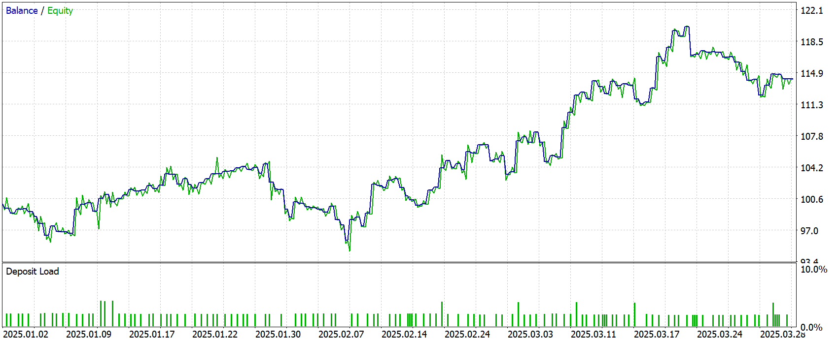
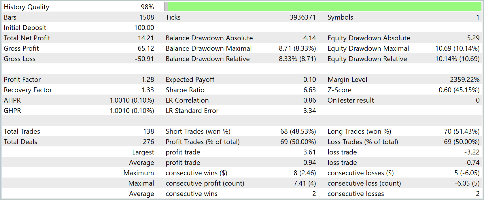
Over the three-month testing period, net profit reached 14.21% of the initial capital. Profit per dollar of loss was $1.28, while the average trade expectancy was only $0.10. A recovery factor of 1.33 indicates that the total profit exceeded the maximum balance drawdown.

The drawdowns appeared moderate: the absolute drawdown was $4.14 by balance and $5.29 by equity, while the maximum relative drawdown was 8.33% and 10.14%, respectively. At the same time, the profit line showed steady growth, as confirmed by a time-based trend correlation of 0.86.

Over the course of the entire test, the Expert Advisor executed 138 trades, divided almost evenly between buys and sells, and the percentage of profitable trades was close to 50% in both directions. The average profit per winning trade was $0.94, the average loss was $0.74, the largest winning trade reached $3.61, and the largest losing trade was $3.22. On average, positions were held for just over an hour, with holding times ranging from 57 minutes to two hours, indicating a distinctly short-term, intraday trading style.

Taken together, the results indicate a fairly stable but moderately profitable strategy. Its strengths include controlled drawdowns, consistent performance in both market directions, and a positive expectancy. Its weaknesses are a limited margin in terms of profit factor and a small average profit per trade, which may make it sensitive to spreads and commissions on a live account.

Conclusion

This article completes the work on implementing the approaches of the HimNet framework using MQL5. The framework's key advantages are its architectural flexibility and its ability to adapt to a wide range of tasks related to time series forecasting and analysis.

The results of final testing on new quotes that were not included in the training set showed positive dynamics. The model's balance demonstrated steady growth, indicating its ability to adapt effectively to changing market conditions.

Links

• Heterogeneity-Informed Meta-Parameter Learning for Spatiotemporal Time Series Forecasting
• Other articles in the series

Programs used in the article

#	Name	Type	Description
1	Study.mq5	Expert Advisor	Expert Advisor for offline model training
2	StudyOnline.mq5	Expert Advisor	Expert Advisor for online model training
3	Test.mq5	Expert Advisor	Expert Advisor for model testing
4	Trajectory.mqh	Class library	Structure describing the system state and model architecture
5	NeuroNet.mqh	Class library	Class library for creating a neural network
6	NeuroNet.cl	Library	Code library for an OpenCL program