Neural Networks in Trading: The Temporal Query Model (Conclusion)

Introduction

The TQNet framework is one of the most elegant and flexible approaches to building neural network models capable of effectively processing time series and structurally organized data. Its key advantage lies in its ability to combine local and global dependencies, creating a distinctive balance between depth of analysis and computational efficiency. Unlike traditional architectures, TQNet seamlessly integrates mechanisms for sequential data processing with methods for capturing long-term dependencies. This is particularly valuable when working with financial time series, where both instantaneous fluctuations and trends that unfold over time are important.

The algorithm is based on an original approach to organizing computations. The global correlation tensor plays a central role in these computations. It creates a kind of map of the relationships between the elements of the sequence, allowing the model to capture local patterns and construct a comprehensive view of the data structure.

The computational process within TQNet can be described as a sequence of coordinated steps. In the first stage, the input data passes through a layer that forms local features, where key characteristics of the current state are extracted. Next, the global correlation mechanism is activated, applying to these features the structural dependencies accumulated over all previous steps. This iterative scheme allows the model to adapt flexibly to changing conditions and account for hidden patterns. What makes this approach unique is that the model is not limited to a rigid data flow order — relationships can form in any direction within the sequence, which expands its capabilities in forecasting and analysis tasks.

The practical value of TQNet becomes apparent when data is subject to noise or has a complex internal structure. Financial markets, weather forecasting, and industrial process analysis — in all these cases, it is not only the accuracy of the forecast that matters, but also the model’s resilience to unexpected outliers and changes in dynamics. Thanks to a well-designed parameter update algorithm and the efficient use of computational resources, TQNet delivers stable performance even on large datasets, without requiring excessive training resources.

The author's visualization of the framework is shown below.

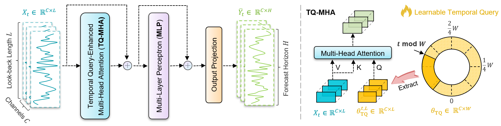
In the previous article, we explored the theoretical aspects of the TQNet framework — its modular architecture, its ability to adapt flexibly to market realities, and its efficient resource management. However, theory is only a skeleton. We also examined the CCircleParams object, which allows global correlations to be stored as objects that can be dynamically switched at each time step. Today, we are continuing our work on implementing the approaches proposed by the authors of the TQNet framework using MQL5.

TQ-MHA Module

The next logical step, which we have reached after successfully implementing the algorithm for organizing the tensor carousel of correlation parameters, is to create the TQ-MHA module. In the authors’ concept, this module plays a special role: it functions as an intelligent filter capable of analyzing the accumulated correlation parameters not in isolation, but in close conjunction with the source data being analyzed. In other words, it processes statistics and tries to capture the living fabric of relationships, supplementing it with the current market context. This approach can be compared to the work of an experienced analyst who does not limit themselves to dry tables and charts, but always puts the numbers to the test by comparing them with real-world events and market dynamics.

If we draw parallels with architectural solutions we are familiar with, TQ-MHA is in many ways similar to a cross-attention module. However, there is a unique aspect to this: instead of a direct comparison of two streams of information — keys and queries—we have a more nuanced process. The TQ-MHA module applies the source data onto correlation-dependency matrices, identifying the most significant intersections. This is not merely a technical optimization, but a qualitatively new level of analysis that allows the framework to interpret market signals within a broader context.

There is another interesting point worth noting here. In the cross-attention modules we have previously implemented according to the principles of transformer architectures, there has always been a FeedForward block — a compact but important element that acts as a nonlinear data transformer between attention layers, whereas the authors of the TQNet framework formally omit this block, as if leaving an entire step of the familiar chain out of the picture. At first glance, this may seem like an oversimplification, but upon closer examination of the framework’s internal logic, we discovered that TQ-MHA is followed by an MLP module, which essentially replicates the full functionality of a classic FeedForward block.

The only difference is in one detail: the activation functions. However, this is not an obstacle for us — on the contrary, it opens up opportunities for experimentation. We can easily replace the activation function with one that better suits our objectives and the specific characteristics of our financial time series.

Thus, we have moved on to designing the specialized CNeuronTQMHA object, which integrates cross-attention logic while taking into account accumulated correlation parameters and ensures seamless interaction with the framework’s other modules. The structure of the new class is shown below.

class CNeuronTQMHA   :  public CNeuronCrossAttention
  {
protected:
   uint              iTimeframe;
   CCircleParams     cParams;
   //---
   virtual bool      feedForward(CNeuronBaseOCL *NeuronOCL, CBufferFloat *SecondInput);
   virtual bool      calcInputGradients(CNeuronBaseOCL *prevLayer, CBufferFloat *SecondInput,
                       CBufferFloat *SecondGradient, ENUM_ACTIVATION SecondActivation = None);
   virtual bool      updateInputWeights(CNeuronBaseOCL *NeuronOCL, CBufferFloat *SecondInput);

public:
                     CNeuronTQMHA(void) {};
                    ~CNeuronTQMHA(void) {};
   //---
   virtual bool      Init(uint numOutputs, uint myIndex, COpenCLMy *open_cl,
                          uint window, uint window_key, uint heads,
                          uint units_in, uint period, uint timeframe,
                          ENUM_OPTIMIZATION optimization_type, uint batch);
   //---
   virtual int       Type(void)   const   {  return defNeuronTQMHA;   }
   //--- methods for working with files
   virtual bool      Save(int const file_handle);
   virtual bool      Load(int const file_handle);
   //---
   virtual bool      WeightsUpdate(CNeuronBaseOCL *source, float tau) override;
   virtual void      SetOpenCL(COpenCLMy *obj);
  }; 

The CNeuronTQMHA class inherits the basic core functionality and most of its internal objects from the CNeuronCrossAttention cross-attention object. However, unlike the basic cross-attention variant, it is designed to work with correlation parameters obtained from the tensor carousel.

Within the class body, we declare only two key elements. The first is iTimeframe, which fixes the time-step size for switching the correlation matrix in our carousel. The second is cParams, an instance of the CCircleParams class, which is responsible for the accumulated correlation parameters. It is precisely these parameters that become the raw material that the multi-head attention will analyze in the context of the initial data.

The internal objects in our class are declared statically, so the constructor and destructor can remain empty — nothing extra happens when the object is created or destroyed. All heavy operations have been moved to the initialization method. This provides clean and predictable object-lifecycle semantics: creation is inexpensive, and preparation for operation is controlled and explicit.

The Init method performs several important steps and carefully checks the result of each one.

bool CNeuronTQMHA::Init(uint numOutputs, uint myIndex, COpenCLMy *open_cl,
                        uint window, uint window_key, uint heads,
                        uint units_count, uint period, uint timeframe,
                        ENUM_OPTIMIZATION optimization_type, uint batch)
  {
   if(!CNeuronCrossAttention::Init(numOutputs, myIndex, open_cl, window,
                                   window_key, heads, units_count, window,
                                   units_count, optimization_type, batch))
      return false;

First, control is passed to the parent class method of the same name, thereby inheriting and configuring the basic cross-attention logic. If the basic initialization fails for any reason, the method immediately returns false — this early exit prevents an invalid state from being propagated further down the stack and simplifies debugging.

Next, we set the activation function between the layers of the FeedForward block.

FF[0].SetActivationFunction(GELU);

As discussed above, the MLP used by the framework’s authors after TQ-MHA essentially serves as a classic FeedForward block. Changing the activation function also makes it possible to flexibly adapt the nonlinearity to the specifics of financial time series. GeLU provides a smoother approximation and often behaves more stably on noisy data than hard ReLU activations. Instantaneous market impulses do not break such a function as harshly, which means training becomes smoother.

The iTimeframe parameter is protected by a lower bound — this is a simple but important safeguard: the parameter value cannot fall to zero. In practice, this means that even with an erroneous configuration, the module will operate in a minimally reasonable mode.

   iTimeframe = MathMax(1, timeframe);
   if(!cParams.Init(0, 0, OpenCL, window * units_count, period, optimization, iBatch))
      return false;
   if(!cParams.Zeros())
      return false;
//---
   return true;
  }

A key part of the initialization process is preparing the cParams object. Here, we explicitly create an internal framework of global correlations. For each time window (window) and for each analyzed univariate sequence (units_count), a corresponding element is created in the correlation tensor. Initialization binds these buffers to the OpenCL context, which ensures further efficiency when handling large amounts of data.

Finally, calling cParams.Zeros sets the initialization strategy recommended by the authors: all global memory parameters are zeroed. This is an important design decision: zero initialization removes any initial biases in the correlations and gives the model a clean slate, on which it builds its own relationships based solely on the training data. This approach is often preferable to random initialization in problems where we do not want to introduce unwanted noise at the memory parameter level.

If all steps are successful, the method returns true: the object is fully ready for use; the buffers have been created, the activation function has been set, and the periodic memory is ready and cleared. Overall, this method provides a stable, predictable, and efficient platform for subsequent operations, where CNeuronTQMHA will actually begin linking the accumulated θ-vectors with the data being analyzed and learning from historical quotes.

After describing the class structure, it is natural to move on to analyzing its key procedure — the forward-pass algorithm. The method begins with the simplest, yet most fundamental, step: verifying that the pointer to the SecondInput buffer is valid.

bool CNeuronTQMHA::feedForward(CNeuronBaseOCL *NeuronOCL, CBufferFloat *SecondInput)
  {
   if(!SecondInput)
      return false;

In this buffer, we expect to receive a reference point for positioning the correlation-parameter carousel. If it is missing, execution is immediately terminated, and false is returned. This check protects the module from invalid calls and prevents further unnecessary calculations.

Next, we determine the current position in the carousel. To do this, we read the element at index zero from the SecondInput buffer. In practice, we expect this to be the open time of the last bar.

   int pos = int(SecondInput[0]);
   pos = (pos / int(iTimeframe)) % cParams.GetPeriod();
   if(!cParams.SetPosition(pos) ||
      !cParams.FeedForward())
      return false;

The resulting integer value is then converted into an index for the parameter carousel. First, by dividing by iTimeframe, we group consecutive steps into buckets of the specified step size — this gives us the block number. Next, the remainder from division by the data period length gives the index of a specific element in the correlation-parameter carousel. Together, these two operations implement the concept of periodic memory: for points in time that lie within the same block and are separated by the period length, the same set of TQ-vectors will be used.

The next block strictly switches the active parameter replica and runs a forward pass through it, during which the correlation parameters are prepared for use. If an error occurs in even one of these steps, the method returns false. This behavior ensures that from this point on we always work with a properly prepared set of global parameters.

The following steps replicate the operation of the cross-attention module. And we could pass control to the identically named method of the parent class, but semantically this creates a problem. In the base implementation, residual connections run along the Query backbone. In our case, Query is not a local representation of the current window, but accumulated TQ vectors — that is, global memory. If we route this same memory through the residual-connection path, we risk overwriting the current local Key/Value signal and suppressing important features coming from the input data. In financial markets, this will quickly become apparent: the model will start relying more on the historical framework and respond worse to fresh impulses, and accuracy will drop.

Therefore, we deliberately reuse the low-level logic for attention computation, but implement our own logic for residual connections and result normalization. This preserves the influence of current data while simultaneously using global TQ knowledge when calculating attention weights.

Once the global correlation vectors have been activated and prepared, we project them into the Query space.

   if(!Q_Embedding.FeedForward(cParams.AsObject()))
      return false;
//---
   if(!KV_Embedding.FeedForward(NeuronOCL))
      return false;

Here, Q_Embedding performs a linear projection of global correlations and distributes them across the attention heads.

At the same time, keys and values are generated based on the source data received from an external program. As a result, two streams emerge: global queries that carry the “memory” of long-term dependencies, and local Key/Value streams that reflect current market behavior.

The next call to the inherited attentionOut method is responsible for computing multi-head attention. At this stage, a standard MHA operation is performed. The result is a per-head attention matrix aggregated into the shared MHAttentionOut buffer.

It is important that what is implemented here is precisely the logic of combining the global (Query from θTQ) and the local (Key/Value from the source data) — this is the heart of the TQ approach.

   if(!attentionOut())
      return false;
//---
   if(!W0.FeedForward(GetPointer(MHAttentionOut)))
      return false;
//---
   if(!SumAndNormilize(W0.getOutput(), NeuronOCL.getOutput(), AttentionOut.getOutput(), iWindow))
      return false;

After the attention results are obtained, they pass through the output projection. This is the very W^O matrix that combines the outputs of all attention heads back into the dimensionality of the original data space.

Next, the data from the two information streams are summed, and the resulting values are normalized. This is a standard step for residual connections. The source data tensor is added to the attention projection, after which the result is normalized over the iWindow window. This design stabilizes the learning process, retains input information, and prevents signal attenuation. Normalization also serves here to protect against distribution drift, which is critical for financial time series with variable volatility.

Next, the MLP block sequence is executed.

   if(!FF[0].FeedForward(GetPointer(AttentionOut)))
      return false;
   if(!FF[1].FeedForward(GetPointer(FF[0])))
      return false;
//---
   if(!SumAndNormilize(FF[1].getOutput(), AttentionOut.getOutput(), Output, iWindow))
      return false;
//---
   return true;
  }

These are two layers of a multilayer perceptron with an intermediate nonlinearity (in our implementation, we used GeLU). In essence, these layers serve the same purpose as the traditional FeedForward layer in transformers: they expand the representation, introduce nonlinearity, amplify useful features, and adjust the frequency range at which the model listens to the signal.

Finally, the second call to SumAndNormilize combines the output of MLP with the previous representation, normalizes it, and produces the final result. This step completes the full processing cycle: from extracting global TQ vectors to obtaining an adapted and normalized representation for the next level of the model.

If all steps were successful, the method returns true, indicating that the forward pass was completed correctly and the results are ready to be used.

An important architectural detail is the sequence of early checks and early error returns: they conserve resources and prevent inconsistent operations with OpenCL buffers, which is critical in production environments.

Transitioning smoothly from the discussion of the forward pass, let’s move on to the mirror stage — the distribution of error gradients within CNeuronTQMHA. Here, we follow the reverse order of computations: from the block’s outputs back to the input data, carefully accumulating error signals and distributing them across all components — the MLP, Attention, the projections, and the global cParams memory.

bool CNeuronTQMHA::calcInputGradients(CNeuronBaseOCL *prevLayer,
                                      CBufferFloat *SecondInput,
                                      CBufferFloat *SecondGradient,
                                      ENUM_ACTIVATION SecondActivation = None)
  {
   if(!prevLayer)
     return false;

In the body of the method, we immediately verify that the pointer to the source data object is valid. This step provides a simple but critically important safeguard. If there is no previous layer, the meaningless computation chain must not be continued.

Next, we start peeling off the gradients from the end of the MLP chain. The internal parameters of the MLP receive the correct error contribution, and the gradients are carefully prepared for transmission further down the chain.

   if(!FF[0].CalcHiddenGradients(FF[1].AsObject()))
      return false;
   if(!AttentionOut.CalcHiddenGradients(FF[0].AsObject()))
      return false;

The following line of code transfers the signal from the MLP back to the point where the MLP received its data: AttentionOut. In other words, we tell the attention block: here is the part of the error attributable to the operation of the MLP; distribute it across your inputs. This ensures consistency between the nonlinear refinement of the representation and the representation itself, formed by Attention.

But before moving on, we need to compute the error gradients of the second information stream of the residual connections, forming the gradient for the W0 projection and passing it further down.

   if(!SumAndNormilize(FF[1].getGradient(), AttentionOut.getGradient(), W0.getGradient(),
                                                                         iWindow, false))
      return false;
   if(!MHAttentionOut.CalcHiddenGradients(W0.AsObject()))
      return false;
   if(!AttentionInsideGradients())
      return false;

The next step moves the gradient into the multi-head attention output that was formed before the W⁰ projection. In other words, we “unwind” the W⁰ projection: its gradient has already been computed, and now we need to know which errors reach the attention heads themselves.

The call to AttentionInsideGradients is a key operation for parsing the internal details of Attention. Here, gradients are computed with respect to all internal components of the attention mechanism and, ultimately, to the Query, Key, and Value tensors. This step is responsible for transforming the aggregated error signal from the space of aggregated attention heads into separate contributions for global Queries and local Keys/Values.

Next, we pass the accumulated gradients back toward the source data (prevLayer is the local input). We call the appropriate method to correctly distribute the error across the weights and prepare the gradients for prevLayer itself.

   if(!prevLayer.CalcHiddenGradients(KV_Embedding.AsObject()))
      return false;
   if(!cParams.CalcHiddenGradients(Q_Embedding.AsObject()))
      return false;

In parallel, we mirror the handling of global memory: the gradients obtained for Queries (Query) are passed to cParams. Thus, training affects not only the local projections but also the parameters of the global correlation memory itself: θTQ neatly receives its share of the error, which will then be used to update the weights.

After splitting the contributions, we need to supplement the error gradient of the source data with values from the input-data backbone. But first, we will scale them by the derivative of the activation function of the preceding layer. Only after that can the results of the two information streams be summed.

   if(!DeActivation(prevLayer.getOutput(), W0.getPrevOutput(), W0.getGradient(),
                                                                    prevLayer.Activation()))
      return false;
   if(!SumAndNormilize(prevLayer.getGradient(), W0.getPrevOutput(), prevLayer.getGradient(),
                                                                          iWindow_K, false))
      return false;
//---
   return true;
  }

This is an important step: it ensures that the final gradient passed to prevLayer takes into account both the effect of the local input and the contribution of the W⁰ projection, correctly distributed with regard to the normalization applied in the forward pass.

Once all these stages have been successfully completed, the method signals that the gradients have been correctly distributed across all internal components of the module and that it is ready for the weight update step.

Once the error gradients have been carefully distributed across all of the neuron’s internal structures, the next natural and logical step in their practical application is to update the parameters. The updateInputWeights method completes the training cycle. It takes the computed gradients and applies them sequentially to the projections, the MLP, and, most importantly, to the global correlation memory itself.

The modular approach we use allows us to create a fairly concise method for updating parameters. We simply pass control sequentially to the methods of the same name in the internal objects, passing the correct pointers to the corresponding source data buffers.

bool CNeuronTQMHA::updateInputWeights(CNeuronBaseOCL *NeuronOCL, CBufferFloat *SecondInput)
  {
   if(!cParams.UpdateInputWeights())
      return false;
   if(!Q_Embedding.UpdateInputWeights(cParams.AsObject()))
      return false;
   if(!KV_Embedding.UpdateInputWeights(NeuronOCL))
      return false;
   if(!W0.UpdateInputWeights(GetPointer(MHAttentionOut)))
      return false;
   if(!FF[0].UpdateInputWeights(GetPointer(AttentionOut)))
      return false;
   if(!FF[1].UpdateInputWeights(GetPointer(FF[0])))
      return false;
//---
   return true;
  }

The updateInputWeights method is a careful and deliberate conclusion to the training cycle. It ensures that the global correlation memory and all its mappings, along with subsequent transformations, receive correct and consistent updates, which is particularly important for the stable and reliable application of TQNet in financial time series forecasting tasks.

The complete source code for the CNeuronTQMHA class and all of its methods is provided in the attachment.

Model Architecture

After assembling all the key components of the TQNet framework, we move on to the next stage: describing the architecture of the trainable models. As before, our goal is to develop a trading system capable of independently analyzing market conditions and making trading decisions. Training is conducted within the Actor-Critic paradigm, where TQNet acts as the environment state encoder. It forms a compact, informative representation of the current market situation, which the Actor relies on when selecting actions and the Critic uses to evaluate their quality.

Unlike the original version of TQNet, we have expanded the model in terms of data preparation and feature generation: we have added blocks for preprocessing and aggregating contextual information, which improves the system’s robustness and generalization ability. The creation of model architecture descriptions is implemented in the CreateDescriptions method. This method forms the skeletal sequence of layers on which all subsequent training and inference logic is based.

bool CreateDescriptions(CArrayObj *&encoder,
                        CArrayObj *&actor,
                        CArrayObj *&critic
                       )
  {
//---
   CLayerDescription *descr;
//---
   if(!encoder)
     {
      encoder = new CArrayObj();
      if(!encoder)
         return false;
     }
   if(!actor)
     {
      actor = new CArrayObj();
      if(!actor)
         return false;
     }
   if(!critic)
     {
      critic = new CArrayObj();
      if(!critic)
         return false;
     }

The method begins with a simple but important step: if the pointers to the layer containers are null, it creates new objects. This is not just a formality — we guarantee that each of the three architectural blocks will have its own independent collection of layer descriptions, ready to be populated sequentially. This explicit allocation provides transparency. The code that follows can assume that the container exists and does not need to check its validity in multiple places.

Next, we move on to building the Encoder — the central element of our model. We clear the container and add layer descriptions one by one, with each step accompanied by a strict success check: if creating an object or adding it to the array fails for any reason, the method carefully releases the resources and returns an error. This kind of discipline in managing memory and state is useful during debugging and in production — it prevents problems from spreading through the stack.

//--- Encoder
   encoder.Clear();
//--- Input layer
   if(!(descr = new CLayerDescription()))
      return false;
   descr.type = defNeuronBaseOCL;
   uint prev_count = descr.count = (HistoryBars * BarDescr);
   descr.activation = None;
   descr.optimization = ADAM;
   if(!encoder.Add(descr))
     {
      delete descr;
      return false;
     }
//--- layer 1
   if(!(descr = new CLayerDescription()))
      return false;
   descr.type = defNeuronBatchNormWithNoise;
   descr.count = prev_count;
   descr.batch = BatchSize;
   descr.activation = None;
   descr.optimization = ADAM;
   if(!encoder.Add(descr))
     {
      delete descr;
      return false;
     }

The first layer of the Encoder is a CNeuronBaseOCL base neuron layer; the number of neurons is set as the product of HistoryBars * BarDescr. The idea here is clear: we feed a historical window into the network, broken down by descriptive features. This layer does not contain an activation function — it serves as a gateway, a buffer to which we simply pass the input data.

The next block — CNeuronBatchNormWithNoise — preserves the dimensionality of the previous layer but adds normalization and noise regularization. This is not just a cosmetic detail: financial time series are subject to distribution drift and outliers. BatchNorm with noise improves robustness to such anomalies, normalizes the inputs for subsequent layers, and at the same time encourages the model not to overfit to small, random variations.

After normalization, we proceed to transform the temporal structure using CNeuronConcatDiff. This layer collects the history by bars, but does so with an emphasis on differences with a step of (step = 1), providing an explicit representation of the dynamics— not only of the levels, but also of their changes. This technique often gives the model a better representation of trend ticks, momentum, and local reversals.

//--- layer 2
   if(!(descr = new CLayerDescription()))
      return false;
   descr.type = defNeuronConcatDiff;
   prev_count = descr.count = HistoryBars;
   descr.layers = BarDescr;
   descr.step = 1;
   descr.batch = BatchSize;
   descr.optimization = ADAM;
   descr.activation = None;
   if(!encoder.Add(descr))
     {
      delete descr;
      return false;
     }

Next comes the CMamba4CastEmbeding layer, which implements multi-window logic for sinusoidal timestamp embeddings. This gives the model the ability to look simultaneously at short-term and long-term patterns, forming a rich representation of the market state.

//--- layer 3
   if(!(descr = new CLayerDescription()))
      return false;
   descr.type = defMamba4CastEmbeding;
   prev_count = descr.count = HistoryBars;
   descr.window = 2 * BarDescr;
   uint prev_out = descr.window_out = NSkills;
     {
      uint temp[] = {PeriodSeconds(PERIOD_D1), PeriodSeconds(PERIOD_MN1)};
      if(ArrayCopy(descr.windows, temp) < (int)temp.Size())
         return false;
     }
   descr.batch = BatchSize;
   descr.optimization = ADAM;
   descr.activation = None;
   if(!encoder.Add(descr))
     {
      delete descr;
      return false;
     }

Here it is worth noting that the preceding operations were performed in the representation of a multivariate time series. For the TQNet framework to work correctly, however, we need a sequence of univariate time series. Therefore, in the next step we transpose the tensor, rearranging the dimensions for the subsequent application of attention.

//--- layer 4
   if(!(descr = new CLayerDescription()))
      return false;
   descr.type = defNeuronTransposeOCL;
   descr.count = prev_count;
   prev_count = descr.window = prev_out;
   descr.batch = BatchSize;
   descr.optimization = ADAM;
   descr.activation = None;
   if(!encoder.Add(descr))
     {
      delete descr;
      return false;
     }
   prev_out = descr.count;

And now we are approaching the heart of it — the CNeuronTQMHA layer. Here, we specify the period size as 24*7, which corresponds to a calendar week on the H1 timeframe. And the step size corresponds to the number of seconds in one bar of the specified timeframe. We want the TQ carousel to store weekly patterns and pull them in steps of the hourly timeframe.

//--- layer 5
   if(!(descr = new CLayerDescription()))
      return false;
   descr.type = defNeuronTQMHA;
     {
      uint temp[] = {prev_out, 64, 24*7, PeriodSeconds(PERIOD_H1)};
                   // window, window_key, period, timeframe
      if(ArrayCopy(descr.windows, temp) < (int)temp.Size())
         return false;
     }
   descr.step=NHeads;
   descr.count=prev_count;
   descr.batch = BatchSize;
   descr.optimization = ADAM;
   if(!encoder.Add(descr))
     {
      delete descr;
      return false;
     }
   uint count = prev_count;
   uint window = prev_out;

Please note that we use a calendar week (7 days), even if the instrument being analyzed is not traded on weekends. This is a necessary measure, since we calculate the carousel element from the bar open time.

Next comes a convolutional layer with a TANH activation function, which serves to compress and project the resulting representations onto a specified planning horizon. This is the stage where a rich representation is translated into specific predictive signals.

//--- layer 6
   if(!(descr = new CLayerDescription()))
      return false;
   descr.type = defNeuronConvOCL;
   descr.count = prev_count;
   descr.window = prev_out;
   descr.step = prev_out;
   prev_out=descr.window_out = NForecast;
   descr.activation = TANH;
   descr.optimization = ADAM;
   if(!encoder.Add(descr))
     {
      delete descr;
      return false;
     }
//--- layer 7
   if(!(descr = new CLayerDescription()))
      return false;
   descr.type = defNeuronTransposeOCL;
   descr.count = prev_count;
   prev_count = descr.window = prev_out;
   descr.batch = BatchSize;
   descr.optimization = ADAM;
   descr.activation = None;
   if(!encoder.Add(descr))
     {
      delete descr;
      return false;
     }
   prev_out=descr.count;

Then, another transposition is performed to return the data to a multivariate sequence representation similar to the original data.

Another convolution is intended to reduce the dimensionality of the features to the level of the original data.

//--- layer 8
   if(!(descr = new CLayerDescription()))
      return false;
   descr.type = defNeuronConvOCL;
   descr.count = prev_count;
   descr.window = prev_out;
   descr.step = prev_out;
   prev_out=descr.window_out = BarDescr;
   descr.activation = TANH;
   descr.optimization = ADAM;
   if(!encoder.Add(descr))
     {
      delete descr;
      return false;
     }

These convolutional passes act as local aggregators — they accumulate information across the forecast components and produce a representation that is ready for denormalization.

The encoder is completed by the CNeuronRevInDenormOCL layer. This module returns the forecasts to their original scale, restoring the mean and variance of the analyzed data that were removed during preprocessing.

//--- layer 9
   if(!(descr = new CLayerDescription()))
      return false;
   descr.type = defNeuronRevInDenormOCL;
   descr.count = prev_count*prev_out;
   descr.layers = 1;
   if(!encoder.Add(descr))
     {
      delete descr;
      return false;
     }

For financial applications, this is essential: forecasts must be on a scale that is interpretable and suitable for trading and risk calculation.

A single idea runs through the entire construct: first, carefully prepare and normalize the input, then extract dynamic features and embeddings at different scales, then apply TQ-enhanced attention, and finally aggregate and project the predicted values into the original data space with scale restoration.

The architectures of the Actor and Critic models have been carried over unchanged from previous works, and we will not dwell on their detailed discussion here. The complete architectural design of all trainable models is provided in the attachment.

Testing

The training process is structured in two sequential and complementary stages — this provides both a solid foundation and the flexibility needed to operate in real-world market conditions.

In the first, offline stage, we performed thorough training on historical data for the EURUSD pair on the H1 timeframe for the entire year of 2024. This year included a full range of market regimes — calm sideways markets, steady trends, sudden spikes in volatility, and periods of increased noise — making it an excellent training ground for the model.

The second stage is online fine-tuning. Training was implemented in an environment as close as possible to live trading: in the MetaTrader 5 Strategy Tester, the model processed the stream of candlesticks sequentially, just as it would in real time. Online mode reveals completely different properties than batch training: the ability to withstand noise, respond to changes in liquidity, and correctly account for delays and the effect of end-to-end slippage. During fine-tuning, we simulated real execution conditions so that the model's behavior would be predictable when transferred to live trading.

The final — and perhaps the most rigorous — stage was testing on completely out-of-sample data: market quotes from January to March 2025. All model parameters and hyperparameters remained frozen; no additional adjustment to these data was performed. This type of validation provides an objective picture of practical effectiveness: it reflects the algorithm's ability to remain predictable and robust under new conditions.

The test results are shown below.

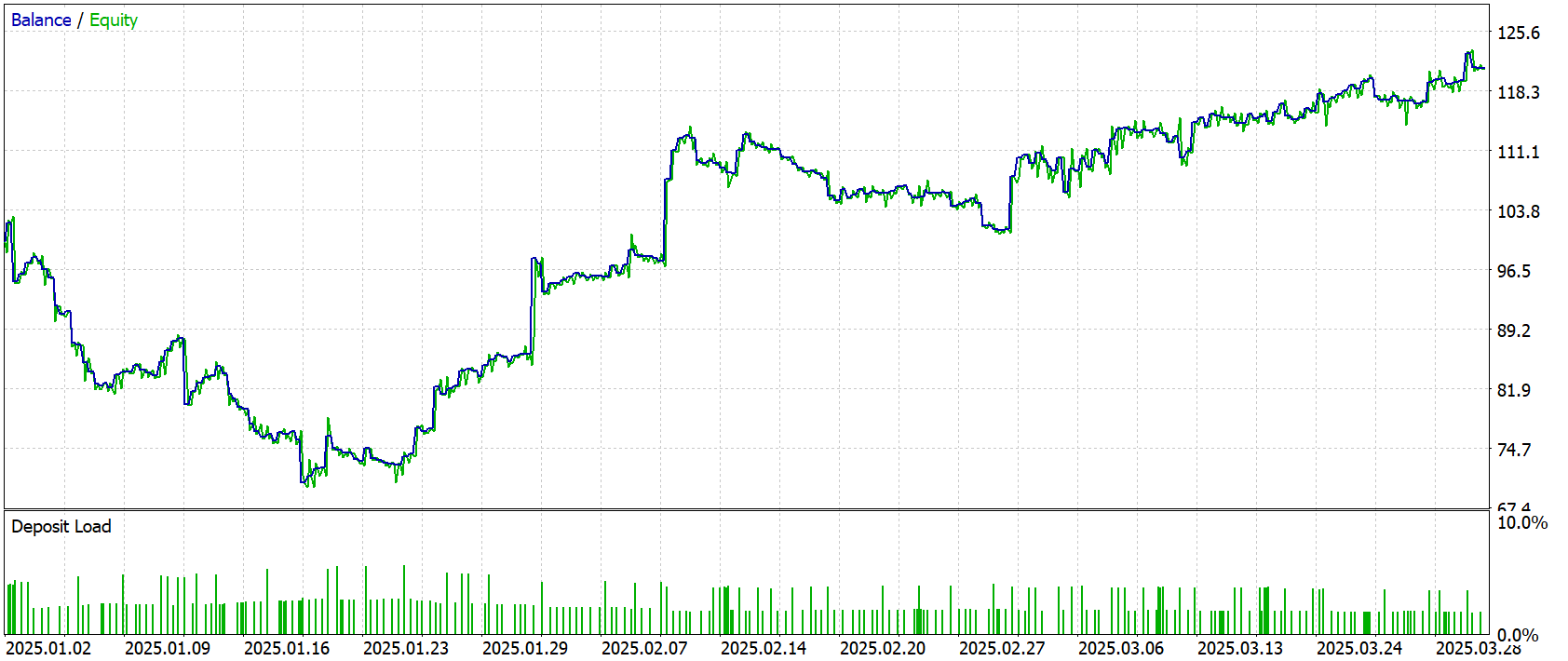
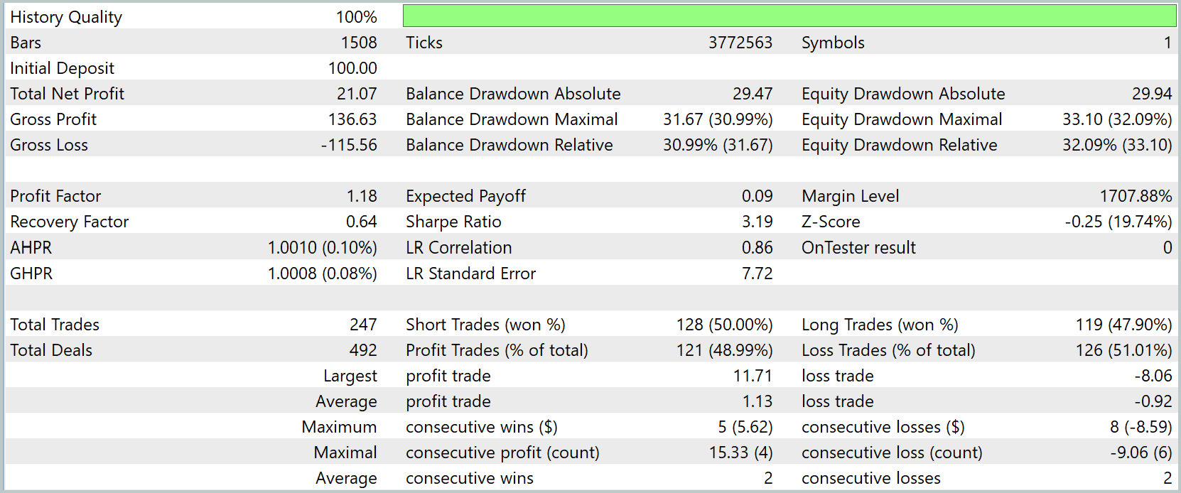
The test results showed a rather subtle positive edge. With an initial deposit of $100, the net profit was $21.07. The share of profitable trades was close to 49%. Moreover, short positions ended in profit slightly more often than long positions. The average profitable trade yielded $1.13, while the average loss was $0.92. A profit factor of 1.18, with an expected return of $0.09 per trade, indicates that the margin of safety is minimal.

Linear regression on the equity curve shows a correlation of 0.86, but the error remains noticeable. This confirms that the results are noisy.

The risk profile is still far from optimal. Deep drawdowns combined with a low expected return per trade make it impossible to grow capital safely. The margin burden is low in this case, which means the problem is not the position size, but the quality of the entry points and exit discipline.

Conclusion

In this paper, we examined in detail the theoretical foundations of the TQNet framework, as well as the specifics of its integration into the architecture of trainable trading models. The key principles underlying the design of the modules, including modified cross-attention mechanisms, were analyzed, making it possible to achieve more flexible and stable algorithm performance under financial market conditions.

In the practical part of the project, we implemented the approaches proposed in TQNet using MQL5, supplementing them with our own improvements in feature generation and data preprocessing. The model was trained in two stages: on historical data (offline training) and under conditions close to the real market (online fine-tuning in the MetaTrader 5 Strategy Tester).

Final testing on new, previously unused price quotes showed positive dynamics. The model's balance showed steady growth after an initial drawdown, indicating the algorithm's ability to adapt to changing market conditions.

The results confirm that TQNet, combined with refined architectural solutions and a two-stage training process, is capable of delivering a positive expected value.

References

• Temporal Query Network for Efficient Multivariate Time Series Forecasting
• Other articles in this series

Programs used in the article

#	Name	Type	Description
1	Study.mq5	Expert Advisor	Expert Advisor for offline model training
2	StudyOnline.mq5	Expert Advisor	Expert Advisor for online model training
3	Test.mq5	Expert Advisor	Expert Advisor for model testing
4	Trajectory.mqh	Class Library	Structure for describing the system state and model architecture
5	NeuroNet.mqh	Class Library	Class library for building a neural network
6	NeuroNet.cl	Library	Code library for the OpenCL program