Integrating MQL5 with Data Processing Packages (Part 10): Deploying Python AutoML Pipelines for Strategy Testing

MetaTrader 5 — Examples | 11 August 2026, 14:15

1 100

Hlomohang John Borotho

Introduction

In the previous part of this series, we explored 'Entropy-Based Adaptive Volatility' model. We now take that foundation further and address a problem every rule-based trader eventually faces. You pick EMA periods, test them, adjust RSI thresholds, test again, and the cycle never ends. Even after all that effort, the strategy still fires signals in conditions where it historically loses. The core issue is that manual optimization cannot distinguish between a crossover that leads to profit and one that leads to a loss. You are treating every signal as equal, even though the market context behind each one is entirely different. The result is a strategy that works on paper but leaks money on signals it should never have taken.

This article solves that problem by introducing an AutoML confidence gate. Instead of hand-tuning parameters, we train a machine learning model on the historical outcomes of every EMA crossover signal. The model learns which market conditions produce profitable trades and which do not. We use FLAML to automatically select and tune the best algorithm, export the trained model to ONNX format, and embed it directly inside an MQL5 Expert Advisor. At runtime, every crossover signal is evaluated by the model before a trade is placed. Only signals the model is confident in get executed.

Model and System Overview

The system begins entirely in Python, inside a Jupyter notebook. We fetch XAUUSD H1 history from MetaTrader 5 and run feature engineering. The pipeline computes nine indicators: two normalized EMAs, their distance, RSI, RSI momentum, normalized ATR, a volatility ratio, close-range percentage, and crossover direction. For every EMA crossover detected in the historical data, a trade is simulated using the next bar's open as entry and the next opposite crossover as exit. Each simulated trade is labeled one if it closed in profit and zero if it did not. These labels become the training target. FLAML then searches across LightGBM, XGBoost, and Random Forest to find the best model automatically. The winning model is exported to ONNX format with a fixed opset and a plain probability tensor output, making it compatible with MetaTrader 5's native ONNX runtime.

The Data Pipeline and Training Phase

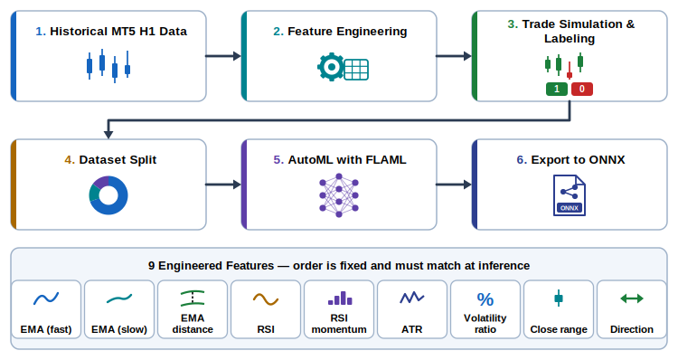
How The Data Pipeline and Training Phase Works:

Load and clean raw OHCL price history.
Derive 9 features from price and indicators.
Simulate each signal, label Profit (1) or Loss (0).
Purge split: 70% train, 15% validation, 15% test.
Search LightGBM, XGBoost, CatBoost and RF.
Save best model with its probability tensor.

The Expert Advisor loads the trained ONNX model as an embedded resource at startup. No external files or Python services are required at runtime. On every new bar, the EA checks whether the fast EMA has crossed the slow EMA on the just-closed bar. If a crossover is detected, it computes the same nine features the model was trained on, in the same order and using matching indicator formulas. These features are passed to the model, which returns a probability that the trade will close in profit. If that probability exceeds the configurable confidence threshold, a market order is placed. Active positions are managed through a combination of an ATR trailing stop and an opposite-crossover exit, mirroring the exit logic used during label generation. The confidence threshold is exposed as an optimizable input, allowing the Strategy Tester to find the value that best balances trade frequency against win rate.

The Live Execution and Trading Phase

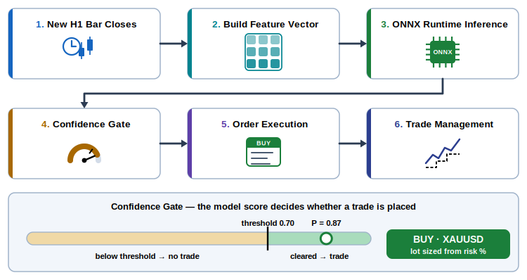
How The Live Execution and Trading Phase Works:

EA wakes on bar close, never mid-bar.
Same 9 features, same order as training.
OnnxRun on the embedded model resource.
Trade only if P (Profit) clears the threshold.
Size the lot from risk %, attach SL and TP.
ATR trailing stop, break-even, then exit.

Getting Started

Environment and Configuration

from datetime import datetime
import sys
import warnings

import pandas as pd
import pytz

warnings.filterwarnings("ignore")

# =============================================================================
#  CONFIG — edit these values
# =============================================================================
SYMBOL      = "XAUUSD"        # exact symbol name as shown in MT5 Market Watch
TIMEFRAME   = "H1"              # M1 M5 M15 M30 H1 H4 D1
DATE_FROM   = datetime(2023, 1,  1)   # start of historical range
DATE_TO     = datetime(2026, 1,  1)   # end   of historical range (exclusive)
OUTPUT_CSV  = "XAUUSD_H1.csv"         # output filename (saved in working directory)
TIMEZONE    = "Etc/UTC"               # keep UTC — pipeline expects UTC timestamps
# =============================================================================

# Timeframe string -> MT5 constant name
TF_MAP = {
    "M1":  "TIMEFRAME_M1",
    "M5":  "TIMEFRAME_M5",
    "M15": "TIMEFRAME_M15",
    "M30": "TIMEFRAME_M30",
    "H1":  "TIMEFRAME_H1",
    "H4":  "TIMEFRAME_H4",
    "D1":  "TIMEFRAME_D1",
}

def fetch():
    try:
        import MetaTrader5 as mt5
    except ImportError:
        sys.exit("[ERROR] MetaTrader5 package not installed.\n"
                 "        Run:  pip install MetaTrader5")

    print(f"MetaTrader5 package  v{mt5.__version__}  by {mt5.__author__}")

    # ── Initialise ───────────────────────────────────────────────────────────
    if not mt5.initialize():
        sys.exit(f"[ERROR] mt5.initialize() failed: {mt5.last_error()}")
    print(f"[MT5]  Connected — build {mt5.version()}")

    # ── Select symbol ────────────────────────────────────────────────────────
    if not mt5.symbol_select(SYMBOL, True):
        mt5.shutdown()
        sys.exit(f"[ERROR] Symbol '{SYMBOL}' not found in Market Watch.\n"
                 "        Check the exact name (e.g. XAUUSD vs XAUUSD.m vs XAUUSDm)")

    info = mt5.symbol_info(SYMBOL)
    point = info.point if info else 0.01
    print(f"[MT5]  Symbol: {SYMBOL}  Point: {point}  Digits: {info.digits if info else '?'}")

    # ── Validate timeframe ───────────────────────────────────────────────────
    tf_attr = TF_MAP.get(TIMEFRAME.upper())
    if tf_attr is None:
        mt5.shutdown()
        sys.exit(f"[ERROR] Unknown timeframe '{TIMEFRAME}'. Choose from: {list(TF_MAP)}")
    tf = getattr(mt5, tf_attr)

    # ── Build UTC-aware date range ───────────────────────────────────────────
    tz      = pytz.timezone(TIMEZONE)
    utc_from = tz.localize(DATE_FROM)
    utc_to   = tz.localize(DATE_TO)
    print(f"[MT5]  Requesting {TIMEFRAME} bars from {utc_from.date()} to {utc_to.date()} ...")

    # ── Fetch ────────────────────────────────────────────────────────────────
    rates = mt5.copy_rates_range(SYMBOL, tf, utc_from, utc_to)
    mt5.shutdown()

    if rates is None or len(rates) == 0:
        sys.exit("[ERROR] No bars returned. Possible causes:\n"
                 "  - Date range has no data for this symbol on this broker\n"
                 "  - Symbol requires a different name (try without .m suffix)\n"
                 "  - MT5 history for this period not downloaded yet\n"
                 "    (Open the chart in MT5 and scroll back to force download)")

    # ── Build DataFrame ──────────────────────────────────────────────────────
    df = pd.DataFrame(rates)
    df["time"] = pd.to_datetime(df["time"], unit="s", utc=True)
    df.set_index("time", inplace=True)

    # Rename tick_volume -> volume, drop spread column if present
    df.rename(columns={"tick_volume": "volume", "real_volume": "real_vol"}, inplace=True)
    keep = [c for c in ["open", "high", "low", "close", "volume"] if c in df.columns]
    df = df[keep].astype(float)

    # ── Quality report ───────────────────────────────────────────────────────
    n_bars     = len(df)
    date_start = df.index[0].strftime("%Y-%m-%d %H:%M")
    date_end   = df.index[-1].strftime("%Y-%m-%d %H:%M")
    price_min  = df["close"].min()
    price_max  = df["close"].max()
    atr_proxy  = (df["high"] - df["low"]).mean()
    gaps       = df.index.to_series().diff().dropna()
    expected   = gaps.mode()[0]
    gap_bars   = (gaps > expected * 1.5).sum()

    print(f"\n{'='*55}")
    print(f"  Data Quality Report")
    print(f"{'='*55}")
    print(f"  Bars fetched   : {n_bars:,}")
    print(f"  Date range     : {date_start}  ->  {date_end}")
    print(f"  Price range    : {price_min:.2f}  ->  {price_max:.2f}")
    print(f"  Mean ATR (H-L) : {atr_proxy:.2f}")
    print(f"  Missing bars   : {gap_bars:,}  (weekend/holiday gaps expected)")
    print(f"{'='*55}\n")

    if n_bars < 1000:
        print(f"[WARN]  Only {n_bars} bars fetched. Consider extending the date range.\n"
              "        Training needs at least 5,000+ bars for meaningful results.")

    # ── Save ─────────────────────────────────────────────────────────────────
    df.to_csv(OUTPUT_CSV)
    print(f"[OK]   Saved {n_bars:,} bars to '{OUTPUT_CSV}'")
    print(f"       File size: {pd.io.common.get_handle(OUTPUT_CSV,'r').handle.seek(0,2) if False else ''}"
          f"{round(Path(OUTPUT_CSV).stat().st_size / 1024, 1)} KB")
    print(f"\nNext step: set csv_file = '{OUTPUT_CSV}' in the training pipeline.")
    return df


# ── Entrypoint ────────────────────────────────────────────────────────────────
from pathlib import Path

if __name__ == "__main__":
    fetch()
else:
    # When imported or run as a Jupyter cell, execute immediately
    fetch()

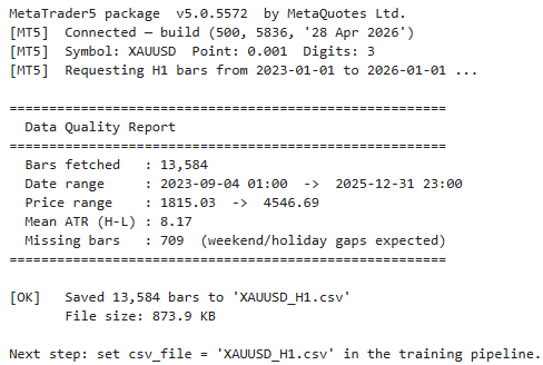
We begin by importing the libraries required to communicate with MetaTrader 5, manipulate data, and manage dates and time zones. Next, we define a configuration section where we specify the trading symbol, timeframe, historical date range, output filename, and timezone that will be used throughout the data collection process. We also create a mapping between readable timeframe names and their corresponding MetaTrader 5 constants to simplify timeframe selection. The fetch() function then initializes the MetaTrader 5 terminal, verifies that the requested symbol and timeframe are valid, and downloads the historical price data for the specified period. Once the data has been retrieved, we convert it into a Pandas DataFrame, format the timestamps in UTC, retain only the required OHLCV columns, and generate a brief data quality report.

import warnings
warnings.filterwarnings("ignore")

import numpy as np
import pandas as pd

# =============================================================================
#  CONFIG — the single source of truth for the whole pipeline
# =============================================================================
CSV_FILE        = "XAUUSD_H1.csv"   # produced by the fetch script (Step 1)

# --- Strategy parameters (must match the MQL5 EA inputs exactly) ---
EMA_FAST        = 12
EMA_SLOW        = 26
RSI_PERIOD      = 14
ATR_PERIOD      = 14
VOL_FAST        = 20      # short std-dev window for volatility_ratio
VOL_SLOW        = 100     # long  std-dev window for volatility_ratio

# --- Labeling ---
MAX_HOLD_BARS   = 50      # exit at next opposite crossover OR after this many bars

# --- Training ---
TEST_FRACTION   = 0.20    # chronological hold-out (most recent 20% of signals)
FLAML_TIME_SEC  = 180     # 3-minute AutoML budget
RANDOM_SEED     = 42

# --- Export ---
ONNX_FILE       = "ema_rsi_model.onnx"
ONNX_OPSET      = 12      # MT5's ONNX runtime safe zone — do NOT raise casually

# --- Feature contract (ORDER IS LAW — the MQL5 EA must fill its input
#     array in exactly this order) ---
FEATURES = [
    "ema_fast_rel",      # 0: EMA(12)/close - 1
    "ema_slow_rel",      # 1: EMA(26)/close - 1
    "ema_distance",      # 2: (EMA fast - EMA slow)/close
    "rsi",               # 3: Wilder RSI(14), 0..100
    "rsi_momentum",      # 4: RSI[0] - RSI[1]
    "atr_rel",           # 5: ATR(14)/close
    "volatility_ratio",  # 6: std(close,20)/std(close,100)
    "close_range_pct",   # 7: (close-low)/(high-low) of the signal bar
    "signal_direction",  # 8: +1 buy crossover, -1 sell crossover
]
N_FEATURES = len(FEATURES)
print(f"Feature contract locked: {N_FEATURES} features")

Next, we define the global configuration that will be used consistently throughout the entire machine learning pipeline. We begin by specifying the historical CSV file generated in the previous step, followed by the trading strategy parameters, including the EMA, RSI, ATR, and volatility settings that must exactly match those used by the MQL5 Expert Advisor. We then configure the trade labeling rules, the AutoML training parameters, and the ONNX export settings to ensure compatibility with MetaTrader 5's native ONNX runtime. Finally, we define the complete feature contract, listing the nine input features in the exact order expected by both the Python training pipeline and the MQL5 Expert Advisor. Maintaining this fixed feature order is essential, as any mismatch between the training model and the EA would produce incorrect predictions during live inference.

Load the Historical Data

df = pd.read_csv(CSV_FILE, index_col="time", parse_dates=True)

required = {"open", "high", "low", "close", "volume"}
missing  = required - set(df.columns)
assert not missing, f"CSV missing columns: {missing}"
assert df.index.is_monotonic_increasing, "Bars are not in chronological order"
assert not df.index.duplicated().any(),  "Duplicate timestamps found"

print(f"Bars loaded : {len(df):,}")
print(f"Date range  : {df.index[0]}  ->  {df.index[-1]}")
df.tail(3)

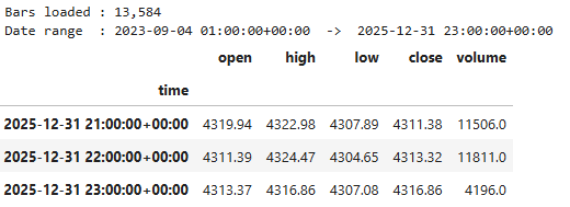
Here, we load the historical price data from the CSV file into a Pandas DataFrame, using the time column as the index and automatically parsing it as datetime values. Before proceeding, we perform several validation checks to ensure the dataset is suitable for model training. We verify that all required OHLCV columns are present, confirm that the bars are arranged in chronological order, and ensure there are no duplicate timestamps that could compromise the analysis.

Feature Engineering

def ema(s: pd.Series, period: int) -> pd.Series:
    # Matches MT5 MODE_EMA
    return s.ewm(span=period, adjust=False).mean()

def rsi_wilder(close: pd.Series, period: int) -> pd.Series:
    # Matches MT5 iRSI (Wilder smoothing) after warm-up
    delta = close.diff()
    gain  = delta.clip(lower=0.0)
    loss  = (-delta).clip(lower=0.0)
    avg_gain = gain.ewm(alpha=1.0 / period, adjust=False).mean()
    avg_loss = loss.ewm(alpha=1.0 / period, adjust=False).mean()
    rs = avg_gain / avg_loss.replace(0.0, np.nan)
    return (100.0 - 100.0 / (1.0 + rs)).fillna(50.0)

def atr_wilder(df: pd.DataFrame, period: int) -> pd.Series:
    # Matches MT5 iATR (Wilder smoothing) after warm-up
    prev_close = df["close"].shift(1)
    tr = pd.concat([
        df["high"] - df["low"],
        (df["high"] - prev_close).abs(),
        (df["low"]  - prev_close).abs(),
    ], axis=1).max(axis=1)
    return tr.ewm(alpha=1.0 / period, adjust=False).mean()


feat = df.copy()

ema_f = ema(feat["close"], EMA_FAST)
ema_s = ema(feat["close"], EMA_SLOW)

feat["ema_fast_rel"]     = ema_f / feat["close"] - 1.0
feat["ema_slow_rel"]     = ema_s / feat["close"] - 1.0
feat["ema_distance"]     = (ema_f - ema_s) / feat["close"]
feat["rsi"]              = rsi_wilder(feat["close"], RSI_PERIOD)
feat["rsi_momentum"]     = feat["rsi"].diff()
feat["atr_rel"]          = atr_wilder(feat, ATR_PERIOD) / feat["close"]
feat["volatility_ratio"] = (feat["close"].rolling(VOL_FAST).std()
                            / feat["close"].rolling(VOL_SLOW).std())
rng = (feat["high"] - feat["low"])
feat["close_range_pct"]  = ((feat["close"] - feat["low"]) / rng).where(rng > 0, 0.5)

# Raw EMA columns kept ONLY for crossover detection — they are NOT model features
feat["_ema_f"] = ema_f
feat["_ema_s"] = ema_s

# Drop the warm-up region (recursive smoothers + 100-bar rolling window)
feat = feat.iloc[200:].dropna(subset=[f for f in FEATURES if f != "signal_direction"])
feat = feat.reset_index()   # positional indexing from here on

print(f"Bars after warm-up trim: {len(feat):,}")
feat[["close", "ema_distance", "rsi", "atr_rel", "volatility_ratio"]].describe().round(4)

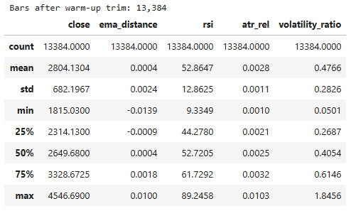
In this section, we compute the technical indicators that will serve as inputs to our machine learning model. We begin by implementing custom functions for the EMA, RSI, and ATR using Wilder's smoothing so that their values closely match those produced by MetaTrader 5. Using these functions, we calculate the normalized EMA values, the distance between the two EMAs, the RSI and its momentum, the normalized ATR, the volatility ratio, and the close-range percentage. We also retain the raw EMA values solely for detecting crossover signals, although they are not included as model features. Then, we remove the initial warm-up period required by the recursive indicators and rolling calculations, discard any remaining incomplete rows, and reset the index to produce a clean feature dataset that is ready for signal generation and trade labeling.

Label Generation

f_arr  = feat["_ema_f"].to_numpy()
s_arr  = feat["_ema_s"].to_numpy()
open_  = feat["open"].to_numpy()
close  = feat["close"].to_numpy()

# Crossover detection at the close of bar i
above     = f_arr > s_arr
cross_up  = above & ~np.roll(above, 1)
cross_dn  = ~above & np.roll(above, 1)
cross_up[0] = cross_dn[0] = False

signal = np.zeros(len(feat), dtype=int)
signal[cross_up] = 1
signal[cross_dn] = -1

sig_idx = np.where(signal != 0)[0]
sig_idx = sig_idx[sig_idx < len(feat) - MAX_HOLD_BARS - 1]   # no truncated trades

records = []
for i in sig_idx:
    direction = signal[i]
    entry     = open_[i + 1]                     # enter at next bar's open

    # Exit: next opposite crossover within the window, else time-stop
    window = signal[i + 1 : i + 1 + MAX_HOLD_BARS]
    opp    = np.where(window == -direction)[0]
    exit_i = (i + 1 + opp[0]) if len(opp) else (i + MAX_HOLD_BARS)

    pnl   = (close[exit_i] - entry) * direction
    records.append({
        "bar":       i,
        "direction": direction,
        "hold_bars": exit_i - i,
        "pnl":       pnl,
        "label":     int(pnl > 0),
    })

trades = pd.DataFrame(records)

print(f"Signals simulated : {len(trades):,}")
print(f"  Buys / Sells    : {(trades.direction == 1).sum():,} / {(trades.direction == -1).sum():,}")
print(f"  Baseline win %  : {trades.label.mean() * 100:.1f}%   <- what the model must beat")
print(f"  Avg hold (bars) : {trades.hold_bars.mean():.1f}")
trades.head()

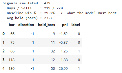
Here, we generate the historical trade labels that our AutoML model will learn from. We begin by detecting bullish and bearish EMA crossover signals using the raw EMA values computed in the previous step. For each crossover, we simulate a trade by entering at the open of the following bar and exiting either at the next opposite crossover or after the maximum holding period has been reached. We then calculate the profit or loss for every simulated trade and assign a binary label, where 1 represents a profitable trade and 0 represents a losing trade. Finally, we store the simulated trade information in a new DataFrame and display summary statistics, including the number of buy and sell signals, the baseline win rate, and the average holding period. These labeled trades form the target dataset that will be used to train our machine learning model.

X = feat.loc[trades["bar"], [f for f in FEATURES if f != "signal_direction"]].reset_index(drop=True)
X["signal_direction"] = trades["direction"].astype(float)
X = X[FEATURES]                       # enforce the contract order
y = trades["label"].to_numpy()

assert list(X.columns) == FEATURES, "Feature order violated!"
assert X.isna().sum().sum() == 0,   "NaNs in the feature matrix!"

print(f"X shape: {X.shape}   |   positive labels: {y.mean()*100:.1f}%")
X.describe().T[["min", "mean", "max"]].round(4)

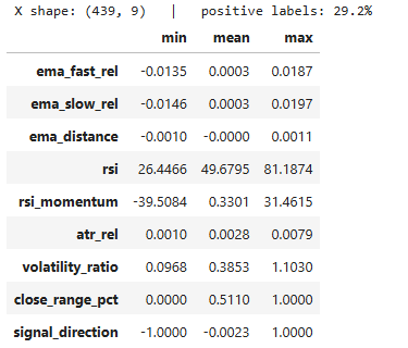
To assemble the training matrix, we extract the feature values corresponding to every simulated trade signal and combine them into a single dataset. We first select the eight computed technical features from the bars where trades were generated, then append the trade direction as the ninth feature to complete our predefined feature contract. Next, we reorder the columns to ensure they exactly match the sequence expected by both the Python training pipeline and the MQL5 Expert Advisor, while storing the trade labels as the target variable. Before proceeding, we verify that the feature order has not changed and confirm that the training matrix contains no missing values.

AutoML Training with FLAML

from flaml import AutoML

split          = int(len(X) * (1 - TEST_FRACTION))
X_train, X_test = X.iloc[:split], X.iloc[split:]
y_train, y_test = y[:split],      y[split:]

print(f"Train signals: {len(X_train):,}   Test signals: {len(X_test):,} (most recent)")

automl = AutoML()
automl.fit(
    X_train=X_train,
    y_train=y_train,
    task="classification",
    metric="roc_auc",
    time_budget=FLAML_TIME_SEC,
    estimator_list=["lgbm", "xgboost", "rf"],
    eval_method="holdout",
    split_type="time",
    seed=RANDOM_SEED,
    verbose=1,
)

best_model = automl.model.estimator     # the underlying sklearn-API model
print("\n" + "=" * 55)
print(f"  Best estimator : {automl.best_estimator}")
print(f"  Best val AUC   : {1 - automl.best_loss:.4f}")
print(f"  Best config    : {automl.best_config}")

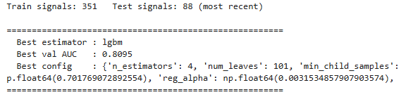
In this section, we train our machine learning model using FLAML's AutoML framework. We begin by splitting the dataset chronologically into training and testing sets, reserving the most recent signals for evaluation so that the model is assessed on unseen market conditions. Next, we initialize the AutoML object and configure it to perform a classification task using the ROC-AUC metric, while allowing it to automatically search for the best-performing model within a fixed time budget. During this search, FLAML evaluates multiple algorithms, including LightGBM, XGBoost, and Random Forest, and optimizes their hyperparameters using a time-aware holdout validation strategy. Once the search is complete, we retrieve the best-performing model and display its selected algorithm, validation AUC score, and optimal hyperparameter configuration.

from sklearn.metrics import roc_auc_score, accuracy_score

proba = best_model.predict_proba(X_test)[:, 1]    # P(trade closes in profit)

print(f"Hold-out AUC      : {roc_auc_score(y_test, proba):.4f}")
print(f"Hold-out accuracy : {accuracy_score(y_test, (proba > 0.5).astype(int)):.4f}")
print(f"Baseline win rate : {y_test.mean()*100:.1f}%  (take every crossover)\n")

print(f"{'Threshold':>9} | {'Trades kept':>11} | {'Win rate':>8} | {'Lift':>6}")
print("-" * 45)
for thr in [0.50, 0.55, 0.60, 0.65, 0.70]:
    mask = proba > thr
    if mask.sum() == 0:
        print(f"{thr:>9.2f} | {'0':>11} |     n/a  |   n/a"); continue
    wr   = y_test[mask].mean()
    lift = wr - y_test.mean()
    print(f"{thr:>9.2f} | {mask.sum():>11,} | {wr*100:>7.1f}% | {lift*100:>+5.1f}%")

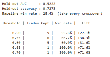
To evaluate on the hold-out dataset, we use the trained model to generate the probability that each test trade will close in profit. We then calculate the ROC-AUC score to measure how well the model separates winning trades from losing trades, and compute the classification accuracy using a default probability threshold of 0.5. For comparison, we also display the baseline win rate that would have been achieved by taking every EMA crossover signal without any machine learning filter. Finally, we test several confidence thresholds ranging from 0.50 to 0.70 and report how many trades would be kept, the resulting win rate, and the performance lift relative to the baseline strategy. This allows us to see how increasing the model's confidence requirement affects both trade frequency and trading quality.

# Which features carry the signal?
import matplotlib.pyplot as plt

imp = pd.Series(best_model.feature_importances_, index=FEATURES).sort_values()
ax = imp.plot(kind="barh", figsize=(8, 4), title=f"Feature importance — {automl.best_estimator}")
ax.set_xlabel("importance")
plt.tight_layout(); plt.show()

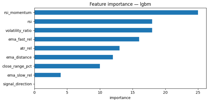
In this section, we examine which input features contribute most to the model's predictions by visualizing their feature importance scores. We begin by retrieving the importance values from the best-performing model and associating each score with its corresponding feature name. The features are then sorted in ascending order to improve readability before being displayed as a horizontal bar chart using Matplotlib. This visualization allows us to identify which market characteristics have the greatest influence on the model's decision-making process, providing valuable insight into how the AutoML model distinguishes profitable trading opportunities from unprofitable ones.

Export to ONNX

import os
from pathlib import Path
from skl2onnx import convert_sklearn, update_registered_converter
from skl2onnx.common.data_types import FloatTensorType
from skl2onnx.common.shape_calculator import calculate_linear_classifier_output_shapes
from onnxmltools.convert.lightgbm.operator_converters.LightGbm import convert_lightgbm
from onnxmltools.convert.xgboost.operator_converters.XGBoost import convert_xgboost
from lightgbm import LGBMClassifier
from xgboost import XGBClassifier

# --- Output path (MT5 Files folder for your terminal) ---
MT5_FILES_DIR = Path(r"C:\Users\...\AppData\Roaming\MetaQuotes\Terminal\...\MQL5\Files\AutoML")
MT5_FILES_DIR.mkdir(parents=True, exist_ok=True)   # creates AutoML folder if it doesn't exist
ONNX_PATH = MT5_FILES_DIR / ONNX_FILE              # full save path

update_registered_converter(
    LGBMClassifier, "LightGbmLGBMClassifier",
    calculate_linear_classifier_output_shapes, convert_lightgbm,
    options={"nocl": [True, False], "zipmap": [True, False]},
)
update_registered_converter(
    XGBClassifier, "XGBoostXGBClassifier",
    calculate_linear_classifier_output_shapes, convert_xgboost,
    options={"nocl": [True, False], "zipmap": [True, False]},
)

onnx_model = convert_sklearn(
    best_model,
    initial_types=[("input", FloatTensorType([None, N_FEATURES]))],
    target_opset={"": ONNX_OPSET, "ai.onnx.ml": 2},
    options={id(best_model): {"zipmap": False}},
)

for op in onnx_model.opset_import:
    if op.domain in ("", "ai.onnx"):
        op.version = ONNX_OPSET

with open(ONNX_PATH, "wb") as f:
    f.write(onnx_model.SerializeToString())

print(f"[OK] Exported to '{ONNX_PATH}'  ({os.path.getsize(ONNX_PATH)/1024:.1f} KB, opset {ONNX_OPSET})")
print("     Inputs :", [(i.name, i.type) for i in onnx_model.graph.input])
print("     Outputs:", [o.name for o in onnx_model.graph.output])

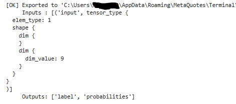
In the final stage of the Python pipeline, we export the trained AutoML model to the ONNX format so it can be executed directly inside MetaTrader 5. We begin by importing the libraries required for ONNX conversion and defining the output directory within the terminal's MQL5\Files folder, creating it automatically if it does not already exist. Next, we register the LightGBM and XGBoost converters to ensure these models can be translated into the ONNX format. We then convert the best-performing model using the predefined feature count and target ONNX opset, while disabling the zipmap output to produce a simple probability tensor that is fully compatible with MetaTrader 5's native ONNX runtime. Finally, we save the serialized model to disk and display the export location, file size, and the model's input and output definitions, confirming that the ONNX model is ready to be loaded by our MQL5 Expert Advisor.

Validate the ONNX Model

import onnxruntime as ort

sess = ort.InferenceSession(ONNX_PATH, providers=["CPUExecutionProvider"])  # <-- ONNX_PATH not ONNX_FILE
input_name = sess.get_inputs()[0].name

X32 = X_test.to_numpy().astype(np.float32)
outputs = sess.run(None, {input_name: X32})

onnx_proba = outputs[1][:, 1]
max_diff   = np.abs(onnx_proba - proba).max()

print(f"Samples validated : {len(X32):,}")
print(f"Max |ONNX - sklearn| probability diff: {max_diff:.2e}")
assert max_diff < 1e-3, "ONNX output diverges from the trained model!"
print("[OK] ONNX model is numerically faithful — safe to deploy to MT5")

# =============================================================================
#  FEATURE CONTRACT — pin this next to your keyboard while writing the EA
# =============================================================================
print(f"ONNX file        : {ONNX_FILE}")
print(f"Input tensor     : '{input_name}'  float32  shape (1, {N_FEATURES})")
print(f"Output tensor #1 : probabilities, float32, shape (1, 2) -> read [0][1] = P(profit)")
print(f"Confidence gate  : EA input parameter (suggested default from the threshold table)")
print()
print(f"{'Idx':>3} | {'Feature':<17} | MQL5 computation")
print("-" * 78)
contract = [
    ("ema_fast_rel",     f"iMA(EMA,{EMA_FAST}) / close[1] - 1.0"),
    ("ema_slow_rel",     f"iMA(EMA,{EMA_SLOW}) / close[1] - 1.0"),
    ("ema_distance",     "(emaFast - emaSlow) / close[1]"),
    ("rsi",              f"iRSI({RSI_PERIOD}) on bar 1"),
    ("rsi_momentum",     "rsi[1] - rsi[2]"),
    ("atr_rel",          f"iATR({ATR_PERIOD}) / close[1]"),
    ("volatility_ratio", f"StdDev(close,{VOL_FAST}) / StdDev(close,{VOL_SLOW})"),
    ("close_range_pct",  "(close[1]-low[1]) / (high[1]-low[1]), 0.5 if flat bar"),
    ("signal_direction", "+1.0 buy crossover, -1.0 sell crossover"),
]
for i, (name, mql) in enumerate(contract):
    print(f"{i:>3} | {name:<17} | {mql}")
print()
print("NOTE: 'bar 1' = the just-closed bar. The EA computes features on the closed")
print("      signal bar and enters on the current bar — mirroring the simulation.")

Before deploying the model to MetaTrader 5, we verify that the exported ONNX model produces the same predictions as the original scikit-learn model. We begin by loading the ONNX model using ONNX Runtime and creating an inference session with the CPU execution provider. Next, we convert the test feature matrix to the float32 format expected by ONNX and perform inference to obtain the predicted probabilities. These probabilities are then compared with those generated by the original trained model, and we calculate the maximum absolute difference between the two outputs. If this difference falls within a small numerical tolerance, we can confidently conclude that the ONNX model faithfully reproduces the behavior of the original model and is safe to deploy inside the MQL5 Expert Advisor.

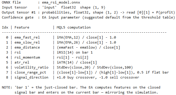
After validating the model, we summarize the feature contract that the Expert Advisor must follow during live inference. We display the ONNX file name, the expected input tensor, the output tensor containing the probability of a profitable trade, and the configurable confidence threshold that will be used as the trade filter. Finally, we print a reference table listing each feature in its exact input order alongside the corresponding MQL5 calculation.

Putting it all Together on MQL5

//+------------------------------------------------------------------+
//|                                              AutoML Pipeline.mq5 |
//|                                  Copyright 2025, MetaQuotes Ltd. |
//|                     https://www.mql5.com/en/users/johnhlomohang/ |
//+------------------------------------------------------------------+
#property copyright "Copyright 2025, MetaQuotes Ltd."
#property link      "https://www.mql5.com/en/users/johnhlomohang/"
#property version   "1.00"

#include <Trade\Trade.mqh>
#resource "\\Files\\AutoML\\ema_rsi_model.onnx" as uchar ExtModelBuffer[]

//+------------------------------------------------------------------+
//| Inputs                                                           |
//+------------------------------------------------------------------+
input group "=== Strategy (must match Python training config) ==="
input int      InpEmaFast       = 12;      // Fast EMA period
input int      InpEmaSlow       = 26;      // Slow EMA period
input int      InpRsiPeriod     = 14;      // RSI period
input int      InpAtrPeriod     = 14;      // ATR period
input int      InpVolFast       = 123;      // StdDev short window
input int      InpVolSlow       = 864;     // StdDev long window
input int      InpMaxHoldBars   = 254;      // Time-stop (bars) — matches labeling

input group "=== AutoML Gate ==="
input bool     InpUseModelGate  = false;    // false = raw EMA+RSI baseline (for A/B tests)
input double   InpConfidence    = 0.55;    // Min P(profit) to take a signal (optimize 0.50–0.75)

input group "=== Risk & Trade Management ==="
input double   InpLots          = 0.36;    // Fixed lot size
input bool     InpUseSL         = true;    // Protective stop-loss
input double   InpSLxATR        = 12.4;     // SL distance = ATR * this
input bool     InpUseTrailing   = true;    // ATR trailing stop (locks in profit)
input double   InpTrailxATR     = 3.0;     // Trail distance = ATR * this
input ulong    InpMagic         = 100010;  // Magic number
input int      InpSlippage      = 7;      // Max deviation (points)

input group "=== Display ==="
input bool     InpShowDashboard = true;    // On-chart status panel

//+------------------------------------------------------------------+
//| Globals                                                          |
//+------------------------------------------------------------------+
#define N_FEATURES 9

CTrade   g_trade;
long     g_onnx        = INVALID_HANDLE;   // ONNX session handle
int      g_hEmaFast    = INVALID_HANDLE;
int      g_hEmaSlow    = INVALID_HANDLE;
int      g_hRsi        = INVALID_HANDLE;
int      g_hAtr        = INVALID_HANDLE;
datetime g_lastBarTime = 0;

//--- Dashboard state
double   g_lastConfidence = 0.0;
string   g_lastSignal     = "none";
string   g_lastDecision   = "-";
int      g_signalsSeen    = 0;
int      g_signalsTaken   = 0;

In MQL5, we begin by including the Trade library to provide access to the CTrade class for order execution and embedding the trained ONNX model as a compiled resource within the Expert Advisor. This approach eliminates the need for external model files during runtime, allowing the EA to load the model directly from its internal resources. Next, we define the input parameters that control the trading strategy, ensuring that the EMA, RSI, ATR, and volatility settings match those used during the Python training process. We also specify the maximum holding period used during trade labeling so that the live trading logic remains consistent with the historical simulations.

The remaining inputs configure the AutoML confidence gate, risk management rules, and on-chart display options. We provide the ability to enable or disable the machine learning filter for performance comparisons, specify the minimum confidence required before executing a trade, and configure the position size, stop-loss, trailing stop, slippage, and magic number used for trade management. Finally, we declare the global variables that will be shared throughout the Expert Advisor. These include the ONNX session handle, indicator handles, the timestamp of the last processed bar, and dashboard variables used to monitor the model's confidence, the most recent trading signal, the final trading decision, and the number of signals detected and executed during operation.

//+------------------------------------------------------------------+
//| Expert initialization                                            |
//+------------------------------------------------------------------+
int OnInit()
  {
//--- Indicator handles 
   g_hEmaFast = iMA(_Symbol, _Period, InpEmaFast, 0, MODE_EMA, PRICE_CLOSE);
   g_hEmaSlow = iMA(_Symbol, _Period, InpEmaSlow, 0, MODE_EMA, PRICE_CLOSE);
   g_hRsi     = iRSI(_Symbol, _Period, InpRsiPeriod, PRICE_CLOSE);
   g_hAtr     = iATR(_Symbol, _Period, InpAtrPeriod);

   if(g_hEmaFast==INVALID_HANDLE || g_hEmaSlow==INVALID_HANDLE ||
      g_hRsi==INVALID_HANDLE     || g_hAtr==INVALID_HANDLE)
     {
      Print("[INIT] Failed to create indicator handles");
      return INIT_FAILED;
     }

//--- ONNX session from the embedded resource 
   g_onnx = OnnxCreateFromBuffer(ExtModelBuffer, ONNX_DEFAULT);
   if(g_onnx == INVALID_HANDLE)
     {
      PrintFormat("[INIT] OnnxCreateFromBuffer failed, error %d", GetLastError());
      return INIT_FAILED;
     }

//--- Pin the shapes. The model was exported with a dynamic batch
//--- dimension (None, 9); MT5 requires it fixed before running.
   const long inShape[]    = {1, N_FEATURES};
   const long outLblShape[]  = {1};
   const long outProbShape[] = {1, 2};

   if(!OnnxSetInputShape(g_onnx, 0, inShape))
     {
      PrintFormat("[INIT] OnnxSetInputShape failed, error %d", GetLastError());
      return INIT_FAILED;
     }
   if(!OnnxSetOutputShape(g_onnx, 0, outLblShape) ||
      !OnnxSetOutputShape(g_onnx, 1, outProbShape))
     {
      PrintFormat("[INIT] OnnxSetOutputShape failed, error %d", GetLastError());
      return INIT_FAILED;
     }

//--- Trade object
   g_trade.SetExpertMagicNumber(InpMagic);
   g_trade.SetDeviationInPoints(InpSlippage);
   g_trade.SetTypeFillingBySymbol(_Symbol);

   PrintFormat("[INIT] OK — model %d bytes embedded, gate=%s, threshold=%.2f",
               ArraySize(ExtModelBuffer),
               InpUseModelGate ? "ON" : "OFF (baseline)",
               InpConfidence);
   return INIT_SUCCEEDED;
  }

//+------------------------------------------------------------------+
//| Expert deinitialization                                          |
//+------------------------------------------------------------------+
void OnDeinit(const int reason)
  {
   if(g_onnx != INVALID_HANDLE)
      OnnxRelease(g_onnx);
   IndicatorRelease(g_hEmaFast);
   IndicatorRelease(g_hEmaSlow);
   IndicatorRelease(g_hRsi);
   IndicatorRelease(g_hAtr);
   Comment("");
  }

In the OnInit function, we create indicator handles for the fast and slow EMAs, the RSI, and the ATR, which will later be used to calculate the same features employed during model training. We verify that each handle has been created successfully before proceeding, ensuring that the EA does not continue with missing or invalid indicators. Next, we create an ONNX inference session directly from the embedded model resource. Since the exported model uses a dynamic input shape, we explicitly define the expected input and output tensor dimensions before inference, allowing MetaTrader 5's ONNX runtime to execute the model correctly.

Once the model has been initialized, we configure the CTrade object by assigning the Expert Advisor's magic number, the maximum allowed slippage, and the appropriate order filling mode for the current symbol. We then print a confirmation message showing that the model has been loaded successfully, along with the current status of the AutoML confidence gate and its configured probability threshold. Finally, the OnDeinit() function performs the necessary cleanup when the Expert Advisor is removed or the terminal is closed. It releases the ONNX session, frees all indicator handles, and clears the on-chart dashboard, ensuring that all allocated resources are properly released before the program terminates.

//+------------------------------------------------------------------+
//| Expert tick                                                      |
//+------------------------------------------------------------------+
void OnTick()
  {
//--- Trailing runs on every tick so profit gets locked intrabar
   if(InpUseTrailing)
      ManageTrailingStop();

//--- Everything else is bar-close logic (mirrors the labeling)
   if(!IsNewBar())
      return;

   ProcessClosedBar();

   if(InpShowDashboard)
      UpdateDashboard();
  }

//+------------------------------------------------------------------+
//| New-bar detector                                                 |
//+------------------------------------------------------------------+
bool IsNewBar()
  {
   datetime t = iTime(_Symbol, _Period, 0);
   if(t == g_lastBarTime)
      return false;
   g_lastBarTime = t;
   return true;
  }

//+------------------------------------------------------------------+
//| Core logic — runs once per bar, on the freshly CLOSED bar        |
//+------------------------------------------------------------------+
void ProcessClosedBar()
  {
//--- 1) Read EMAs on bars 1 (closed) and 2 (prior) 
   double emaF[], emaS[];
   if(CopyBuffer(g_hEmaFast, 0, 1, 2, emaF) < 2)
      return;   // [0]=bar1 [1]=bar2? No:
   if(CopyBuffer(g_hEmaSlow, 0, 1, 2, emaS) < 2)
      return;
//--- CopyBuffer fills as-series=false by default: emaF[0]=bar2, emaF[1]=bar1
   double emaFast1 = emaF[1], emaFast2 = emaF[0];
   double emaSlow1 = emaS[1], emaSlow2 = emaS[0];

//--- 2) Crossover on the closed bar (same rule as Python) 
//---    Python: above[i] != above[i-1]
   bool crossUp = (emaFast1 >  emaSlow1) && (emaFast2 <= emaSlow2);
   bool crossDn = (emaFast1 <= emaSlow1) && (emaFast2 >  emaSlow2);
   int  direction = crossUp ? 1 : (crossDn ? -1 : 0);

//--- 3) Exit management first (mirrors the label simulation)
//---    Exit rule in training: opposite crossover OR time stop
   if(PositionSelectByMagic())
     {
      long   posType  = PositionGetInteger(POSITION_TYPE);
      bool   opposite = (posType==POSITION_TYPE_BUY  && crossDn) ||
                        (posType==POSITION_TYPE_SELL && crossUp);

      datetime openTime = (datetime)PositionGetInteger(POSITION_TIME);
      int barsHeld = iBarShift(_Symbol, _Period, openTime);

      if(opposite)
        {
         g_trade.PositionClose(_Symbol);
         PrintFormat("[EXIT] Opposite crossover after %d bars", barsHeld);
        }
      else
         if(barsHeld >= InpMaxHoldBars)
           {
            g_trade.PositionClose(_Symbol);
            PrintFormat("[EXIT] Time stop hit (%d bars)", barsHeld);
           }
     }

//--- 4) Entry evaluation
   if(direction == 0)
      return;                          // no signal this bar

   g_signalsSeen++;
   g_lastSignal = (direction > 0) ? "BUY cross" : "SELL cross";

   if(PositionSelectByMagic())         // still holding (same-direction cross)
     {
      g_lastDecision = "skipped (position open)";
      return;
     }

//--- 5) Build the feature vector — THE CONTRACT
   float features[N_FEATURES];
   if(!ComputeFeatures(direction, features))
     {
      g_lastDecision = "skipped (feature error)";
      return;
     }

//--- 6) Query the model 
   double pProfit = 1.0;               // gate off => always pass
   if(InpUseModelGate)
     {
      if(!RunModel(features, pProfit))
        {
         g_lastDecision = "skipped (inference error)";
         return;
        }
     }
   g_lastConfidence = pProfit;

   PrintFormat("[SIGNAL] %s | P(profit)=%.3f | threshold=%.2f",
               g_lastSignal, pProfit, InpConfidence);

   if(pProfit <= InpConfidence)
     {
      g_lastDecision = StringFormat("REJECTED (%.3f <= %.2f)", pProfit, InpConfidence);
      return;
     }

//--- 7) Execute 
   ExecuteEntry(direction);
  }

In the OnTick() function, we define the main execution flow of the Expert Advisor. We begin by managing the trailing stop on every incoming tick so that profitable positions can be protected as the market moves. All remaining trading logic is executed only when a new bar is detected, ensuring that the EA behaves exactly like the Python training pipeline, which generates signals using closed candles. The IsNewBar() function detects the formation of a new candle by comparing the latest bar timestamp with the previously processed one, preventing the same signal from being evaluated multiple times. Once a new bar is confirmed, we call ProcessClosedBar() to evaluate trading opportunities and update the on-chart dashboard with the latest model information.

ProcessClosedBar() implements the EA's decision logic. We first retrieve the EMA values from the two most recently closed bars to detect bullish and bearish crossover signals, then manage any existing position by applying the same exit rules used during the Python trade simulations, namely an opposite crossover or the maximum holding period. If a new trading signal is identified and no position is currently open, we compute the nine-feature input vector and, when enabled, pass it to the ONNX model to estimate the probability of a profitable trade. This probability is compared against the user-defined confidence threshold, allowing low-confidence signals to be filtered out before execution. Only signals that satisfy the confidence requirement are forwarded to the order execution routine, ensuring that the live trading logic remains fully consistent with the model training and evaluation pipeline.

//+------------------------------------------------------------------+
//| Feature vector — order and math must match the Python notebook   |
//+------------------------------------------------------------------+
bool ComputeFeatures(const int direction, float &f[])
  {
//--- Prices of the closed bar
   double close1 = iClose(_Symbol, _Period, 1);
   double high1  = iHigh(_Symbol, _Period, 1);
   double low1   = iLow(_Symbol, _Period, 1);
   if(close1 <= 0.0)
      return false;

//--- Indicator values
   double emaF[], emaS[], rsi[], atr[];
   if(CopyBuffer(g_hEmaFast, 0, 1, 1, emaF) < 1)
      return false;
   if(CopyBuffer(g_hEmaSlow, 0, 1, 1, emaS) < 1)
      return false;
   if(CopyBuffer(g_hRsi,     0, 1, 2, rsi) < 2)
      return false;  // rsi[0]=bar2 rsi[1]=bar1
   if(CopyBuffer(g_hAtr,     0, 1, 1, atr) < 1)
      return false;

//--- Sample standard deviations (pandas-compatible, ddof=1).
//--- iStdDev uses the POPULATION formula (ddof=0), which is
//--- systematically ~1–2%% smaller — a silent feature-drift bug.
   double sdFast = StdDevSample(InpVolFast,  1);
   double sdSlow = StdDevSample(InpVolSlow,  1);
   if(sdFast <= 0.0 || sdSlow <= 0.0)
      return false;

   double range1   = high1 - low1;
   double rangePct = (range1 > 0.0) ? (close1 - low1) / range1 : 0.5;

   f[0] = (float)(emaF[0] / close1 - 1.0);            // ema_fast_rel
   f[1] = (float)(emaS[0] / close1 - 1.0);            // ema_slow_rel
   f[2] = (float)((emaF[0] - emaS[0]) / close1);      // ema_distance
   f[3] = (float)(rsi[1]);                            // rsi (bar 1)
   f[4] = (float)(rsi[1] - rsi[0]);                   // rsi_momentum
   f[5] = (float)(atr[0] / close1);                   // atr_rel
   f[6] = (float)(sdFast / sdSlow);                   // volatility_ratio
   f[7] = (float)(rangePct);                          // close_range_pct
   f[8] = (float)(direction);                         // signal_direction

   return true;
  }

//+------------------------------------------------------------------+
//| Sample std-dev                                                   |
//+------------------------------------------------------------------+
double StdDevSample(const int period, const int shift)
  {
   double closes[];
   if(CopyClose(_Symbol, _Period, shift, period, closes) < period)
      return 0.0;

   double mean = 0.0;
   for(int i = 0; i < period; i++)
      mean += closes[i];
   mean /= period;

   double ss = 0.0;
   for(int i = 0; i < period; i++)
     {
      double d = closes[i] - mean;
      ss += d * d;
     }
   return MathSqrt(ss / (period - 1));    // ddof = 1
  }

The ComputeFeatures() function constructs the nine-feature input vector that is passed to the ONNX model for inference. To match training, we compute all features on the just-closed bar using the same formulas as in Python. We begin by retrieving the closed bar's price data, followed by the latest EMA, RSI, and ATR values from their respective indicator buffers. We then compute the short-term and long-term standard deviations, the candle's close-range percentage, and finally populate the feature array in the exact order defined by the feature contract. If any required price or indicator data cannot be retrieved, the function immediately returns false, preventing invalid data from being passed to the model.

Then, the StdDevSample() function supports this process by calculating the sample standard deviation of recent closing prices. Instead of relying on the built-in iStdDev indicator, which uses the population standard deviation, we implement our own calculation using the sample standard deviation (ddof = 1) to match Pandas' default behavior during model training. This seemingly small difference is important because even slight discrepancies between the Python and MQL5 feature calculations can introduce feature drift and lead to inconsistent model predictions. By reproducing the same statistical calculation in both environments, we ensure that the Expert Advisor receives feature values that closely match those used to train the AutoML model.

//+------------------------------------------------------------------+
//| ONNX inference — returns P(trade closes in profit)               |
//+------------------------------------------------------------------+
bool RunModel(const float &features[], double &pProfit)
  {
   long  outLabel[1];        // output 0: predicted class (int64)
   float outProbs[1][2];     // output 1: [P(loss), P(profit)]

   if(!OnnxRun(g_onnx, ONNX_NO_CONVERSION, features, outLabel, outProbs))
     {
      PrintFormat("[ONNX] OnnxRun failed, error %d", GetLastError());
      return false;
     }

   pProfit = (double)outProbs[0][1];
   return true;
  }

//+------------------------------------------------------------------+
//| Entry execution with optional ATR stop-loss                      |
//+------------------------------------------------------------------+
void ExecuteEntry(const int direction)
  {
   double atr[];
   if(CopyBuffer(g_hAtr, 0, 1, 1, atr) < 1)
      return;

   double sl = 0.0;
   bool ok   = false;

   if(direction > 0)
     {
      double ask = SymbolInfoDouble(_Symbol, SYMBOL_ASK);
      if(InpUseSL)
         sl = NormalizeDouble(ask - InpSLxATR * atr[0], _Digits);
      ok = g_trade.Buy(InpLots, _Symbol, 0.0, sl, 0.0, "AutoML gate");
     }
   else
     {
      double bid = SymbolInfoDouble(_Symbol, SYMBOL_BID);
      if(InpUseSL)
         sl = NormalizeDouble(bid + InpSLxATR * atr[0], _Digits);
      ok = g_trade.Sell(InpLots, _Symbol, 0.0, sl, 0.0, "AutoML gate");
     }

   if(ok)
     {
      g_signalsTaken++;
      g_lastDecision = StringFormat("TAKEN (%.3f > %.2f)", g_lastConfidence, InpConfidence);
     }
   else
     {
      g_lastDecision = StringFormat("order failed (%d)", (int)g_trade.ResultRetcode());
      PrintFormat("[TRADE] Order failed: retcode=%d", (int)g_trade.ResultRetcode());
     }
  }

In this section, the RunModel() function is responsible for performing ONNX inference within the Expert Advisor. We begin by allocating memory for the model's outputs, consisting of the predicted class label and the probability scores for both possible outcomes. Next, we pass the nine-feature input vector to the embedded ONNX model using OnnxRun(). If the inference process fails, the function reports the corresponding error code and returns false. Otherwise, we extract the probability that the current trading signal will close in profit from the second element of the output tensor and store it in pProfit, allowing the Expert Advisor to compare this value against the configured confidence threshold before making a trading decision.

The ExecuteEntry() function handles the execution of approved trading signals. We begin by retrieving the latest ATR value, which is used to calculate an optional volatility-based stop-loss. Depending on whether the signal is bullish or bearish, we compute the appropriate stop-loss level relative to the current Ask or Bid price and submit either a buy or sell market order using the CTrade object. After the order request is sent, we check whether it was executed successfully. Successful trades update the dashboard statistics and record that the signal passed the confidence gate, while failed orders generate an informative error message containing the trade server's return code to assist with debugging.

//+------------------------------------------------------------------+
//| ATR trailing stop — the "guarantee the profit" layer             |
//+------------------------------------------------------------------+
void ManageTrailingStop()
  {
   if(!PositionSelectByMagic())
      return;

   double atr[];
   if(CopyBuffer(g_hAtr, 0, 1, 1, atr) < 1)
      return;
   double trail = InpTrailxATR * atr[0];

   long   type    = PositionGetInteger(POSITION_TYPE);
   double sl      = PositionGetDouble(POSITION_SL);
   double openPx  = PositionGetDouble(POSITION_PRICE_OPEN);

   if(type == POSITION_TYPE_BUY)
     {
      double bid   = SymbolInfoDouble(_Symbol, SYMBOL_BID);
      double newSL = NormalizeDouble(bid - trail, _Digits);
      //--- Only trail once in profit, only ever move the stop UP
      if(newSL > openPx && (sl == 0.0 || newSL > sl))
         g_trade.PositionModify(_Symbol, newSL, PositionGetDouble(POSITION_TP));
     }
   else
     {
      double ask   = SymbolInfoDouble(_Symbol, SYMBOL_ASK);
      double newSL = NormalizeDouble(ask + trail, _Digits);
      //--- Only trail once in profit, only ever move the stop DOWN
      if(newSL < openPx && (sl == 0.0 || newSL < sl))
         g_trade.PositionModify(_Symbol, newSL, PositionGetDouble(POSITION_TP));
     }
  }

//+------------------------------------------------------------------+
//| Select the EA's own position on this symbol                      |
//+------------------------------------------------------------------+
bool PositionSelectByMagic()
  {
   for(int i = PositionsTotal() - 1; i >= 0; i--)
     {
      ulong ticket = PositionGetTicket(i);
      if(ticket == 0)
         continue;
      if(PositionGetString(POSITION_SYMBOL) == _Symbol &&
         PositionGetInteger(POSITION_MAGIC) == (long)InpMagic)
         return true;
     }
   return false;
  }

//+------------------------------------------------------------------+
//| On-chart dashboard                                               |
//+------------------------------------------------------------------+
void UpdateDashboard()
  {
   string gate = InpUseModelGate
                 ? StringFormat("ON  (threshold %.2f)", InpConfidence)
                 : "OFF — raw EMA+RSI baseline";

   string pos = "flat";
   if(PositionSelectByMagic())
     {
      long type = PositionGetInteger(POSITION_TYPE);
      int  held = iBarShift(_Symbol, _Period,
                            (datetime)PositionGetInteger(POSITION_TIME));
      pos = StringFormat("%s | %d/%d bars | P/L %.2f",
                         type==POSITION_TYPE_BUY ? "LONG" : "SHORT",
                         held, InpMaxHoldBars,
                         PositionGetDouble(POSITION_PROFIT));
     }

   Comment(StringFormat(
              "\n  EMA+RSI AutoML EA  (Part 10)"
              "\n  --------------------------------------"
              "\n  Model gate      : %s"
              "\n  Last signal     : %s"
              "\n  Last P(profit)  : %.3f"
              "\n  Last decision   : %s"
              "\n  Signals seen    : %d   taken: %d  (%.0f%%)"
              "\n  Position        : %s",
              gate, g_lastSignal, g_lastConfidence, g_lastDecision,
              g_signalsSeen, g_signalsTaken,
              g_signalsSeen > 0 ? 100.0 * g_signalsTaken / g_signalsSeen : 0.0,
              pos));
  }
//+------------------------------------------------------------------+

The ManageTrailingStop() function implements an ATR-based trailing stop to protect profits as the market moves in our favor. We begin by checking whether the Expert Advisor currently has an open position and retrieving the latest ATR value to determine the trailing distance. Depending on whether the position is long or short, we calculate a new stop-loss level relative to the current Bid or Ask price. To avoid increasing risk, the stop-loss is adjusted only after the position has moved into profit, and it is allowed to move in one direction only—upwards for buy positions and downwards for sell positions. This ensures that profits can be locked in while still giving the trade enough room to follow the prevailing market trend.

Then, the PositionSelectByMagic() function helps the Expert Advisor identify and manage only the positions that belong to it by searching for trades with the matching symbol and magic number. The UpdateDashboard() function complements this by providing a real-time summary of the Expert Advisor's activity directly on the chart. It displays the current status of the AutoML confidence gate, the latest trading signal, the model's predicted probability of profit, the resulting trading decision, the number of signals detected and executed, and information about any active position, including its direction, holding period, and current profit or loss.

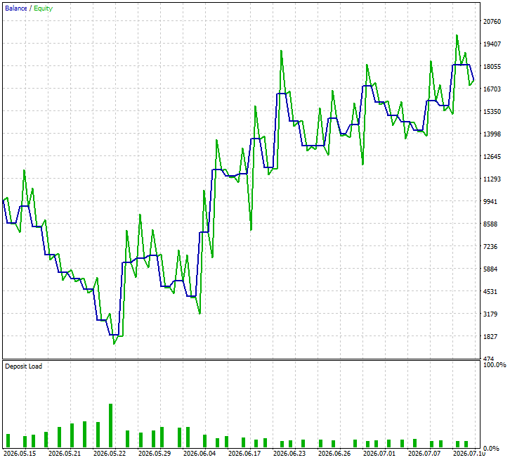
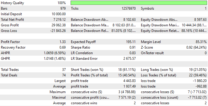
Backtest Results

The backtest was conducted across roughly a 2-month testing window from 15 May 2026 to 15 July 2026, with the default settings:

Conclusion

We began with a problem every rule-based trader faces: a strategy that fires too many signals, with no reliable way to tell the good ones from the bad. To solve it, we built a complete end-to-end pipeline that moves from raw MetaTrader 5 data all the way to a deployed Expert Advisor, with automated machine learning doing the heavy lifting in between. We fetched three years of XAUUSD H1 history, engineered nine market context features, and simulated every EMA crossover as a real trade to generate honest profit-or-loss labels. We then handed that dataset to FLAML and let it automatically search across LightGBM, XGBoost, and Random Forest to find the best model without a single manual hyperparameter decision. We addressed common ONNX export pitfalls: dual-domain opset, zipmap output, and Pandas vs MetaTrader 5 standard-deviation mismatch. As a result, the Python-trained model runs consistently inside the EA.

What the reader walks away with is not just a working strategy. It is a reusable framework. The feature contract, the label generation logic, the FLAML training configuration, and the ONNX deployment pattern are all designed to be adapted. Swap the EMA crossover for any other signal, replace the nine features with your own indicators, and the same pipeline optimizes your strategy automatically. We also demonstrated how to run a genuine A/B test inside the Strategy Tester by toggling the model gate off, giving you a clean way to measure exactly how much the machine learning filter contributes. The confidence threshold becomes an optimizable input, turning a subjective tuning decision into an objective search.

Below is the brief description of what is contained inside the 'AutoML zip':

File Name	File Description
Part10_AutoML_Pipeline.ipynb	A Jupyter notebook for selecting and training an ONNX model.
ema_rsi_model.onnx	The selected best estimator (lgbm) converted to the trained ONNX model.
AutoML Pipeline.mq5	The MetaTrader 5 Expert Advisor that works with the trained ONNX model.

This project is supported in Algo Forge.

Attached files |

Download ZIP

AutoML.zip (39.99 KB)

Warning: All rights to these materials are reserved by MetaQuotes Ltd. Copying or reprinting of these materials in whole or in part is prohibited.

This article was written by a user of the site and reflects their personal views. MetaQuotes Ltd is not responsible for the accuracy of the information presented, nor for any consequences resulting from the use of the solutions, strategies or recommendations described.