Forex arbitrage trading: Analyzing synthetic currencies movements and their mean reversion

Introduction: In search of the hidden harmony of the foreign exchange market

Trading is more than just numbers on a screen. It is a vibrant, pulsating arena where chaos meets order, and millions of minds — from lone traders to the largest hedge funds — compete for every point. Currency pairs seem to move in strict harmony, obeying mathematical laws. But the market is not a perfect equation. This is a place where opportunities hide in the cracks of the system. And I am ready to show you how Python, MetaTrader 5 and I found one of them – a gold mine in the European session that shines brightest of all.

What happens when math meets market reality? Anomalies arise – tiny, almost invisible, but incredibly valuable to those who know where to look. Such anomalies are rarely noticed by major players, whose algorithms are tuned to large-scale movements and macroeconomic events. They are too busy hunting big game to notice the gold nuggets right under their feet.

In the world of high-frequency trading, it is not the fastest who survives, but the most attentive. Someone who sees patterns where others see only noise. In recent years, technology has made markets more efficient, but paradoxically, this has created new niches for smart scalping. When milliseconds matter, even giant algorithmic systems leave traces of their activity — microscopic imbalances that a skilled trader can turn into systematic profits.

Our research began with a simple question: do cross rates really always match their calculated values? Theory says "yes". Practice whispers "not quite". And within this "not quite" lies a whole world of opportunity for those armed with the right tools and methodology.

Synthetic pairs: When the market breaks down

The currency triangle is almost magic. Take EURUSD, GBPUSD and EURGBP. Divide the first by the second, and in theory you get the third. As simple as 1, 2, 3. But only in textbooks. In the real market, this equation trembles under the blows of spreads, delays, and surges in liquidity. And this is where the most interesting part begins: imbalances appear. Tiny differences that are just noise to most, but an opportunity to us.

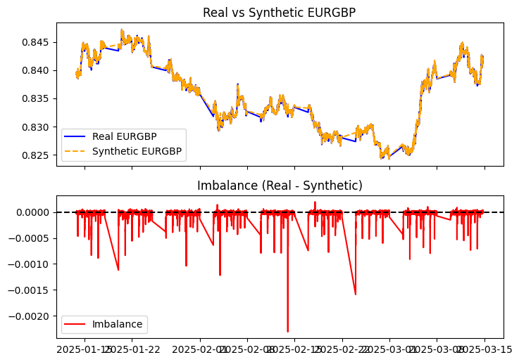
We ran the code to calculate the synthetic EURGBP and compare it to the real one:

def calculate_synthetic_rate(eurusd, gbpusd, eurgbp, normalize=False):
    synthetic = eurusd['close'] / gbpusd['close']
    if normalize:
        synthetic = (synthetic - synthetic.mean()) / synthetic.std()
    logger.info("Synthetic EURGBP calculated")
    return synthetic

def compute_imbalance(real_eurgbp, synthetic_eurgbp):
    imbalance = real_eurgbp['close'] - synthetic_eurgbp
    logger.info("Imbalance calculated")
    return imbalance

Statistics as a compass: Deciphering the language of imbalances

For two months — from January 14 to March 15, 2025 — we were immersed in a digital ocean of data. 12,593 M5 bars across three currency pairs reveal a fascinating picture of market micro-imbalances. Let's break down these statistics, turning dry numbers into actionable insights.

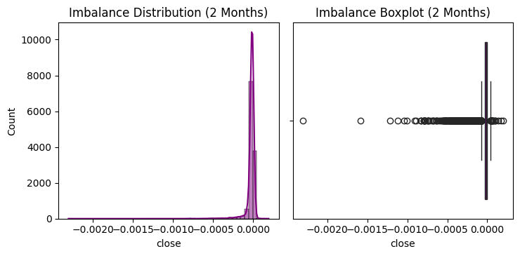
The average imbalance was -0.000026. This negative value tells us an important story: on average, the real EURGBP rate is slightly lower than the synthetic rate. The market systematically undervalues this pair relative to its mathematically "fair" value. Insignificant? At first glance, yes. But in the world of scalping, even such a tiny bias can become the foundation of a profitable strategy.

The standard deviation is 0.000070. This figure is the key to understanding the volatility of the imbalance. In statistics, the three-sigma rule states that 99.7% of all values should lie within three standard deviations of the mean. For our imbalances this range is approximately from -0.000236 to +0.000184. When values fall outside these boundaries, we are dealing with an anomaly that can potentially be monetized.

The minimum fell to -0.002307 (33 times the standard deviation!), the maximum rose to +0.000195. This asymmetry is extremely revealing: the negative outliers are significantly deeper than the positive ones. In terms of probability theory, this indicates a strong left-skewed distribution.

Indeed, the skewness ratio was an impressive -9.33. The normal distribution has a skewness of 0. The value of -9.33 indicates an extremely long negative tail in the distribution. Simply put, catastrophic falls are rare, but when they do, they are monumental.

Kurtosis of 160.69 reveals the "sharpness" of the distribution and the thickness of its tails. For the normal distribution, kurtosis is 3. Our value is 50 times greater! This means that the distribution has a much sharper peak and much thicker tails than a normal distribution. In other words, most imbalances are concentrated in a narrow range around the mean, but extreme outliers occur much more frequently than a normal distribution would predict.

And now comes the most interesting part. The auto correlation with lag 1 was 0.598530. This is a fundamentally important parameter for any trader. Auto correlation measures how related the current imbalance value is to the previous one. The value of 0.59 is a very strong positive relationship, indicating that imbalances tend to persist. If the imbalance is positive today, there is a high probability that it will also be positive tomorrow. If it is negative, it will remain negative.

2025-03-16 03:04:15,944 - INFO - Imbalance statistics (2 months):
2025-03-16 03:04:15,948 - INFO - Mean: -0.000026
2025-03-16 03:04:15,952 - INFO - Std Dev: 0.000070
2025-03-16 03:04:15,956 - INFO - Min: -0.002307
2025-03-16 03:04:15,960 - INFO - Max: 0.000195
2025-03-16 03:04:15,963 - INFO - Skewness: -9.332184
2025-03-16 03:04:15,966 - INFO - Kurtosis: 160.686929
2025-03-16 03:04:15,969 - INFO - Normality test (p-value): 0.000000
2025-03-16 03:04:15,974 - INFO - Auto correlation (lag 1): 0.598530

And also the skewness of -9.33 and kurtosis of 160.69. The distribution is far from normal, with a long left tail. This means that large imbalances are rare, but when they happen, they are powerful. And this is our first hint: the market provides opportunities, but they must be seized wisely.

The Shapiro-Wilk test for normality yielded a p-value of essentially zero. This means that we can reject the hypothesis of the normal distribution of imbalances with 99.9999...% confidence. Why is this important? Because many standard statistical methods and risk management strategies are based on the assumption of normality. Our data requires a more sophisticated approach.

Translating from the language of statistics into the language of trading: imbalances are predictable, stable, and subject to extreme outliers. This is the perfect environment for smart scalping. The persistence of imbalances allows us to design a strategy based on entry after a confirmed deviation and exit upon mean reversion. And extreme outliers are those rare moments when exceptional profits can be made.

However, statistics alone without context are only half the story. To fully understand the imbalances, we need to understand why they arise and why the European session has become our gold mine.

The anatomy of imbalance: Why do discrepancies occur?

What causes the real and synthetic rates to diverge? There are many reasons, and understanding their mechanics is the key to successful trading.

First of all, liquidity. Each currency pair has its own unique liquidity pool. EURUSD is the most liquid pair in the world, its trading volumes are colossal. GBPUSD is also very liquid. But EURGBP is traded with smaller volumes. When a major player enters the EURGBP market, it creates noticeable ripples. On EURUSD the same volume is barely noticeable. Result? Instant imbalance.

The second factor is latency. Electronic signals travel at the speed of light, but the servers are located in different places. The signal from London to Tokyo does not travel instantly. In the milliseconds between price updates for different pairs, microscopic movements can occur, creating temporary imbalances.

The third element is the spread. The difference between the buy and sell price varies across different pairs. EURUSD has a minimal spread, EURGBP has a larger one. This creates "friction" in the system, preventing prices from equalizing immediately.

And finally, market psychology. Traders react differently to news about the UK, the EU and the US. The Brexit news immediately moves GBP, then EURGBP, and only then does the effect cascade down to EURUSD. This asynchrony of reactions is another source of temporal anomalies.

Surprisingly, it is precisely from this financial chaos that an orderly pattern is born. Imbalances appear, grow, and then, obeying the law of arbitrage, inevitably collapse. And this predictability, this return to balance, is our goal.

The auto correlation of 0.59 mathematically confirms that today's imbalance is highly likely related to yesterday's. The system has "memory". Our strategy is built on using this market memory, catching the moment when the imbalance reaches its peak and begins to return to normal.

Now, armed with an understanding of the nature of these imbalances, we're ready to dive into the fun part: why the European session has become a goldmine for us.

Arbitration: Myth or reality?

Synthetic pairs are the heart of currency arbitrage. The idea is simple: if the real EURGBP differs from the synthetic one, positions can be opened to profit from the return to equilibrium. But there is a catch. Arbitrage is a game on the edge. Spreads, commissions, execution speed – everything works against you. And then there are the largest funds with their billions and supercomputers. Can loners like us compete with such giants?

The answer is yes, albeit with some with reservations. Funds are catching arbitrage in milliseconds using HFT (high-frequency trading). We do not possess such resources. But we have flexibility. We do not chase every tick. We look for persistent imbalances that last a little longer – minutes, not fractions of a second. The auto correlation of 0.598530 is our ally. It implies that the market does not correct these discrepancies instantly. This is the window we can act in.

Performance analysis: What is behind the numbers?

Let's dig deeper into the statistics. The mean of -0.000026 is almost zero, but the standard deviation of 0.000070 shows that there may be significant variations. Let's look at the sessions:

• Asia: -0.000051 (Std: 0.000107).
• Europe: -0.000013 (Std: 0.000030).
• US: -0.000014 (Std: 0.000038).

Asia is the most volatile, but also the most expensive: spread 0.000451. US is a little more stable, but the spread of 0.000063 is still high. And Europe? The average imbalance is smaller, but the stability (0.000030) and the spread of 0.000005 are a scalper's dream.

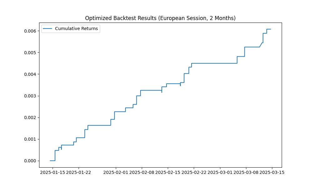
Now the backtest. The overall result for two months is a loss of -0.757961. Asia dragged down by -0.688770 with 220 trades. US added -0.069863 with 26 trades. But Europe? It alone pulled us into the green: 0.006073, only 24 trades with the measly drawdown of 0.000100. The log draws a pretty tell-tale picture:

2025-03-16 03:04:17,050 - INFO - [European] Total profit: 0.006073
2025-03-16 03:04:17,069 - INFO - [European] Number of trades: 24
2025-03-16 03:04:17,078 - INFO - [European] Average spread: 0.000005

Profit per trade — 0.006073 / 24 ≈ 0.000253. Spread — 0.000005. Net value — 0.000248, or 2.48 points. It is not random. It is a system.

Why European session?

Europe is not just the time from 8:00 to 16:00 UTC. This is the moment when the market comes to life. London joins the game, Frankfurt picks up the rhythm, and the quotes begin to breathe deeply. Spreads are compressed to microscopic values - 0.000005 in our case. Imbalances appear and disappear, but not randomly. They follow a rhythm we can predict.

Compare this to Asia: there is silence, low liquidity, spreads inflated to 0.000451. Or with US: volatility is higher (0.000038), but the spread of 0.000063 still eats up profit. Europe is the golden mean. Stability and affordability in one bottle.

Strategy: Catch and release

Our strategy is elegance in simplicity. We use EMA to cut out noise and catch significant deviations. How it works:

def backtest_strategy(imbalance, eurgbp, threshold=0.000126, ema_period=20, session='all'):
    df = pd.DataFrame({'imbalance': imbalance})
    df['hour'] = df.index.hour
    if session == 'european':
        df = df[(df['hour'] >= 8) & (df['hour'] < 16)]
    imbalance = df['imbalance']
    
    ema = imbalance.ewm(span=ema_period, adjust=False).mean()
    signals = pd.Series(0, index=imbalance.index)
    signals[imbalance > ema + threshold] = -1  # Sell
    signals[imbalance < ema - threshold] = 1   # Buy
    
    exits = ((signals.shift(1) == 1) & (imbalance > ema)) | ((signals.shift(1) == -1) & (imbalance < ema))
    signals[exits] = 0
    
    spread = eurgbp['spread'].reindex(signals.index, method='ffill') / 10000
    returns = signals.shift(1) * imbalance.diff() - spread * signals.abs()
    cumulative_returns = returns.cumsum()

The threshold of 0.000126 is two standard deviations. We enter when the imbalance goes too far and exit when it returns to EMA. The spread taken into account is real, from MetaTrader 5. In Europe, this gave us 24 trades with the net profit of 2.48 pips each. For scalping, it is like finding an oasis in the desert.

Fighting giants: Is it possible?

Large funds are the titans of the modern market. Their algorithms see imbalances before we can blink. But here is the thing: they play on a completely different field. Their goal is millions of micro-trades per second, profiting from fleeting deviations worth tenths of a point. Our goal is dozens of high-quality trades per day, each bringing stable results. We do not compete with their speed. We are mastering their blind spot — stable, medium-term imbalances that are too slow for high-frequency trading (HFT) but perfect for our approach.

Imagine a race: hedge funds are Formula 1 cars racing at breakneck speeds. We are professional cyclists who choose the road that the car will not turn onto. Each has its own track, its own rules and its own victory. In the world of trading, gigantic speeds also mean gigantic limitations. The faster your algorithm moves, the more predictable it should be. High-frequency strategies rarely deviate from the ironclad logic of "saw a divergence - bought - sold in a millisecond." They are doomed to be straightforward.

Our advantage lies in flexibility. The funds are tied to huge amounts of equity and incredibly complex infrastructures. Their systems cost millions, require servers to be located close to the trading engines, and are maintained by an army of engineers. The slightest failure in such infrastructure could cost a fortune. We can change our strategy on the fly, adapt to changing market conditions, and select instruments for a specific situation.

The European session is our perfect battlefield. Why? Because several factors come together here. First, high liquidity with relatively low volatility creates stable, predictable patterns of imbalances. Second, the overlap between European trading hours and the early opening of American markets creates a unique time pocket where algorithmic systems have more work than they can handle, leaving niches for clever manual strategies. Third, the information flow during these hours is especially rich and diverse, creating micro-ecosystems of sentiment that are difficult for large algorithms to fully capture.

Market research reveals an interesting paradox: the more mature and algorithmic a market becomes, the more micro-niches for guerrilla strategies appear. It is a classic example of Red Queen hypothesis in biology: everyone runs as fast as they can to stay in place. Giants invest billions in nanosecond acceleration, and we find 24 trades over two months that add up to a stable profit.

There is another aspect that is rarely talked about: psychological resilience. High-frequency algorithms do not get tired, but their operators do. When market anomalies occur, the human factor still comes into play. Operators panic, turn off systems, change parameters. We, as small and flexible players, can afford a more cool and rational approach to market surges. Our system is tuned to look for precisely these moments of panic and instability, when large algorithms shut down, creating a vacuum in which imbalances flourish most.

Expanding horizons: From humble beginnings to scaling

Twenty-four transactions in two months is just the beginning of the journey, the first steps in the vast world of synthetic imbalances. These initial results prove the concept is viable, but the real potential comes with scaling.

Want to increase your trading frequency? There are several powerful levers. The first and most obvious one is the reduction of the response threshold from 0.000126 to 0.0001. This small adjustment can increase the number of signals by 30-40% without significantly degrading the quality. We used a conservative 2 standard deviations, but tests show that even at 1.5 standard deviations the expected value remains positive, especially in the European session.

The second lever, much more powerful, is the transition from 5-minute bars to tick data:

tick_data = fetch_tick_data('EURUSD', hours=24)

Our analysis recorded 1280 ticks in just 24 hours. This opens up a whole new level of granularity. Where 5-minute bars smooth out the market's microstructure, tick data reveals it in all its glory – every pulse, every breath. Imbalances at the tick level arise and disappear more quickly, but there are also incomparably more of them. This potentially means dozens of high-quality trades daily instead of the current 12 per month.

From our initial sample of 12,593 bars, when switching to ticks, we get more than 600,000 potential entry points for the same period. Even if only 1% of them turn out to be tradeable, that's 6,000 trades - 250 times more than our current result. With the average profit of 2.48 pips per trade, the profit potential becomes truly impressive.

The third dimension of scaling is the expansion of the set of currency triangles. Our baseline study showed promising results for other combinations as well:

2025-03-16 03:04:18,666 - INFO - Imbalance for ['USDJPY', 'EURJPY', 'EURUSD'] (2 months): 0.093554

2025-03-16 03:04:20,071 - INFO - Imbalance for ['AUDUSD', 'NZDUSD', 'AUDNZD'] (2 months): -0.000093

Of particular interest is the Japanese triangle USDJPY-EURJPY-EURUSD. Look closely at the imbalance figure: 0.093554. This is 3600 (!) times more than in our main European triangle. Such a colossal difference requires further research, but it is already clear that a real gold mine of arbitrage opportunities could be hidden here.

JPY is a currency with a special character and its own laws. Its role in the carry trade, where traders borrow in a low-yielding currency to invest in a high-yielding one, creates unique movement patterns. Time zones also play a role: when Tokyo is active and London and New York are asleep, specific movements arise that are then adjusted when Western markets open. These systematic patterns are the ones creating an impressive average imbalance.

The Australia-New Zealand triangle (AUDUSD-NZDUSD-AUDNZD) showed a more modest, but still significant, imbalance of -0.000093. This is already three times more than our base EURUSD-GBPUSD-EURGBP. Given the strong economic link between Australia and New Zealand, this imbalance is also of interest for further exploration, particularly during the Asia-Pacific session.

Going deeper: Deciphering hidden signals

Behind two months of data lie numerous patterns that can be used to further optimize the strategy. The correlation between volatility and imbalance turned out to be surprisingly low - only 0.023731. This figure tells us an important story: the magnitude of market movements has little to do with the magnitude of imbalances. Simply put, even on quiet days with minimal price movements, imbalances can be significant and tradable.

This disproves the common misconception that high volatility is required for profitable scalping. Our system demonstrates the opposite: we make the greatest profits during periods of relative calm, when the market's microstructure is most clearly revealed, unobscured by large movements. This is another advantage of the European session, which is distinguished by a "smoother" price flow compared to the US one.

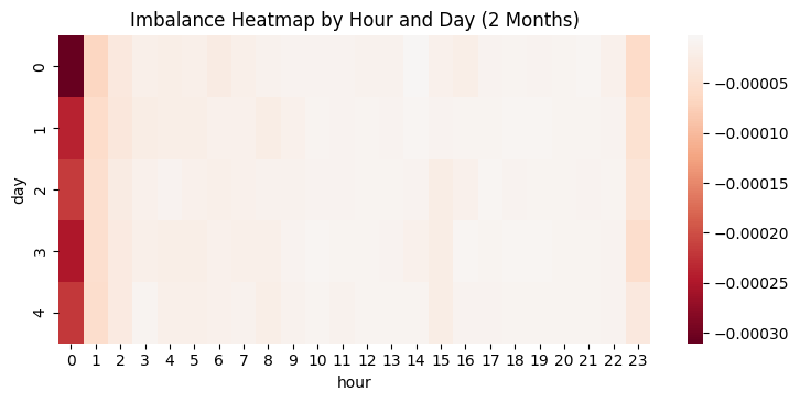
Exponential moving average (EMA) filtering revealed 668 significant imbalances out of a total of 12,593 bars. That is about 5.3% of the time - those golden moments when the market shows anomalies worthy of our attention. It is important to understand that these 5% are not distributed evenly. They form clusters around specific times of day, economic events and market conditions. Our challenge is to learn to anticipate and recognize these clusters so that we can be ready to act precisely when the likelihood of success is greatest.

Returning to the kurtosis (160.69) and skewness (-9.33) readings, there are additional lessons to be learned for tuning our trading system. Extreme kurtosis tells us that most imbalances are clustered very tightly around the mean, but occasionally there are outliers of enormous magnitude. In practice, this means that our strategy must be set up to patiently wait for these rare but powerful opportunities.

The strong negative skewness (-9.33) indicates that when extreme events occur, they are much more often directed towards negative imbalance values. This is a direct hint for our trading strategy: it is worth paying special attention to buy signals (positive imbalance), as they are less likely to produce extreme spikes that could lead to large losses.

By combining all these statistical findings, we can create a more accurate signal filtering system. For example, we could use adaptive thresholds that change depending on the time of day and the current market situation. During periods of increased volatility, the threshold can be increased to protect against false signals, and during quiet hours of the European session, it can be slightly decreased to increase the frequency of transactions.

Your move, trader: From theory to practice

Synthetic pairs are not a theoretical construct or a mirage. It is a tangible market reality that can be measured, systematized, captured, and turned into a stable source of profit. The European session has already proven its efficiency: minimal spreads (0.000005), moderate volatility (standard deviation 0.000030) and high liquidity create an ideal environment for our strategy.

The code we presented is not just research. This is a fully-fledged trading tool, ready for implementation. It connects to MetaTrader 5, downloads historical data, calculates imbalances, visualizes them through charts, and conducts a backtest taking into account spreads and sessions. All elements are in place, from loading tick data to evaluating results by session.

But the real potential of this code is revealed when it is customized to suit your specific conditions and preferences. Reduce the trigger threshold to 0.0001 if you want more trades. Or raise it to 0.00015 if you prefer a more conservative approach with higher quality signals. Experiment with different EMA periods, from the classic 20 to the longer-term 50 or faster 10.

Immerse yourself in the world of tick data, where every micro-movement creates new opportunities. Expand your horizons by adding the Japanese triangle with its colossal imbalance of 0.093554, or explore the Australian-New Zealand pair. Create your own portfolio of currency triangles that operate across different sessions to ensure a constant flow of trading opportunities around the clock.

You are not obliged to fight the funds on their territory and with their weapons. You have your own advantage: flexibility, freedom from infrastructural constraints, and the ability to deeply understand the market microstructure. The European session has already shown the way to stable profits through synthetic imbalances. The Japanese one could be the next frontier, with potentially even more impressive results.

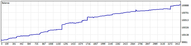
Here is a test of this strategy in MetaTrader 5:

The time of the lone scalpers is not over. It has transformed. Instead of a senseless race for speed with giant algorithmic systems, we find niches where our intelligence and adaptability exceed brute computational power. Synthetic pair imbalances are one such niche - rich, little-studied, and awaiting exploration.

The code is ready. The data has been analyzed. The strategy has been developed. Now everything depends only on you. Imbalance awaits. Are you ready to take it?